is to correlate in software instead of custom-built hardware, ... important advantages and disadvantages. ... For educational purposes, we made the correlator.
BUILDING CORRELATORS WITH MANY-CORE HARDWARE Rob V. van Nieuwpoort and John W. Romein Stichting ASTRON (Netherlands Institute for Radio Astronomy) Oude Hoogeveensedijk 4, 7991 PD Dwingeloo, The Netherlands {nieuwpoort,romein}@astron.nl ABSTRACT Radio telescopes typically consist of multiple receivers whose signals are cross-correlated to filter out noise. A recent trend is to correlate in software instead of custom-built hardware, taking advantage of the flexibility that software solutions offer. Examples include e-VLBI and LOFAR. However, the data rates are usually high and the processing requirements challenging. Many-core processors are promising devices to provide the required processing power. In this paper, we explain how to implement and optimize signal-processing applications on multi-core CPUs and manycore architectures, such as the Intel Core i7, NVIDIA and ATI GPUs, and the Cell/B.E. We use correlation as a running example. The correlator is a streaming, possibly real-time application, and is much more I/O intensive than applications that are typically implemented on many-core hardware today. We compare with the LOFAR production correlator on an IBM Blue Gene/P supercomputer. We discuss several important architectural problems which cause architectures to perform suboptimally, and also deal with programmability. The correlator on the Blue Gene/P achieves a superb 96% of the theoretical peak performance. We show that the processing power and memory bandwidth of current GPUs are highly imbalanced. Because of this, the correlator achieves only 16% of the peak on ATI GPUs, and 32% on NVIDIA GPUs. The Cell/B.E. processor, in contrast, achieves an excellent 92%. Many of the insights we discuss here are not only applicable to telescope correlators, are valuable when developing signal-processing applications in general. 1. INTRODUCTION Radio telescopes produce enormous amounts of data. The Low-Frequency Array (LOFAR) [1], for instance, will produce some tens of petabits per day, and the Australian SKA Pathfinder will even produce over six exabits per day [2]. These modern radio telescopes use many separate receivers as building blocks, and combine their signals to form a single large and sensitive instrument. To extract the sky signal from the system noise, the correlator correlates the signals from different receivers, and integrates the correlations over time, to reduce the amount of data.
This is a challenging problem in radio astronomy, since the data volumes are large, and the computational demands grow quadratically with the number of receivers. Correlators are not limited to astronomy, but are also used in geophysics [3], radar systems [4], wireless networking [5], etc. Traditionally, custom-built hardware, and later FPGAs were used to correlate telescope signals. A recent development is to use a supercomputer [6]. Both approaches have important advantages and disadvantages. Custom-built hardware is efficient and consumes modest amounts of power, but is inflexible, expensive to design, and has a long development time. Solutions that use a supercomputer are much more flexible, but are less efficient, and consume more power. Future instruments, like the Square Kilometre Array (SKA), need several orders of magnitude more computational resources. It is likely that the requirements of the SKA cannot be met by using current supercomputer technology. Therefore, it is important to investigate alternative hardware solutions. General-purpose architectures no longer achieve performance improvements by increasing the clock frequency, but by adding more compute cores and by exploiting parallelism. Intel’s recent Core i7 processor is a good example of this. It has four cores and supports additional vector parallelism. Furthermore, the high-performance computing community is steadily adopting clusters of Graphics Processor Units (GPUs) as a viable alternative to supercomputers, due to their unparalleled growth in computational performance, increasing flexibility and programmability, high power efficiency, and low purchase costs. GPUs are highly parallel and contain hundreds of processor cores. An example of a processor that combines GPU and CPU qualities into one design is the Cell Broadband Engine [7]. The Cell/B.E. consists of an “ordinary” PowerPC core and eight powerful vector processors that provide the bulk of the processing power. Programming the Cell/B.E. requires more effort than programming an ordinary CPU, but various studies showed that the Cell/B.E. performs well on signal-processing tasks like FFTs [8]. In this article, we explain how many-core architectures can be exploited for signal-processing purposes. We give insights into their architectural limitations, and how to best cope with them. We treat five different, popular architectures with multiple cores: the Cell/B.E., GPUs from both
NVIDIA and ATI, the Intel Core i7 processor, and the IBM Blue Gene/P (BG/P) supercomputer. We discuss their similarities and differences, and how the architectural differences affect optimization choices and the eventual performance of a correlator. We also discuss the programmability of the architectures. We focus on correlators, but many of the findings, claims, and optimizations hold for other signal-processing algorithms as well, both inside and outside the area of radio astronomy. For instance, we discuss another signal-processing algorithm, radio-astronomy imaging, on many-core hardware elsewhere [9]. In this paper, we use the LOFAR telescope as a running example, and use its production correlator on the BG/P as a comparison. This way, we demonstrate how many-core architectures can be used in practice for a real application. For educational purposes, we made the correlator implementations for all architectures available online. They exemplify the different optimization choices for the different architectures. The code may be reused under the GNU public license. We describe and analyze the correlator on many-core platforms in much more detail in [10]. 2. TRENDS IN RADIO ASTRONOMY During the past decade, new types of radio-telescope concepts emerged that rely less on concrete, steel, and extreme cooling techniques, but more on signal-processing techniques. For example, LOFAR [1], MeerKAT (Karoo Array Telescope) [11] and ASKAP (Australian Square Kilometre Array Pathfinder) [2] are distributed sensor networks that combines the signals of many receiver elements. All three are pathfinders for the future SKA (Square Kilometre Array) [12] telescope, which will be orders of magnitude larger. These instruments combine the advantages of higher sensitivity, higher resolution, and multiple concurrent observation directions. But, they require huge amounts of processing power to combine the data from the receiving elements. The signal-processing hardware technology used to process telescope data also changes rapidly. Only a decade ago, correlators required special-purpose ASICs to keep up with the high data rates and processing requirements. The advent of sufficiently fast FPGAs significantly lowered the developments times and costs of correlators, and increased the flexibility substantially. LOFAR requires even more flexibility to support many different processing pipelines for various observation modes, and uses FPGAs for on-the-field processing and a BG/P supercomputer to perform real-time, central processing. We describe LOFAR in more detail below. 2.1. The LOFAR telescope LOFAR is an aperture array radio telescope operating in the 10 to 250 MHz frequency range [1]. It is the first of a new generation of radio telescopes, that breaks with the concepts of traditional telescopes in several ways. Rather than using
Fig. 1. A field with LOFAR antennas.
large, expensive dishes, LOFAR uses many thousands of simple antennas that have no movable parts, see Figure 1. Essentially, it is a distributed sensor network that monitors the sky and combines all signals centrally. This concept requires much more signal processing, but the costs of the silicon for the processing are much lower that the costs of steel that would be needed for dishes. Moreover, LOFAR can observe the sky in many directions concurrently and switch directions instantaneously. In several ways, LOFAR will be the largest telescope of the world. The antennas are simple, but there are a lot of them: 44000 in the full LOFAR design. To make radio pictures of the sky with adequate resolution, these antennas are to be arranged in clusters. In the rest of this paper, we call a cluster of antenna’s a receiver. The receivers will be spread out over an area of ultimately 350 km in diameter. This is shown in Figure 3. Data transport requirements are in the range of many tera-bits/sec and the processing power needed is tens of tera-ops. Another novelty is the elaborate use of software to process the telescope data in real time. LOFAR thus is an ITtelescope. The cost is dominated by the cost of computing and will follow Moore’s law, becoming cheaper with time and allowing increasingly large telescopes to be built. LOFAR will enable exciting new science cases. First, we expect to see the Epoch of Reionization (EoR), the time that the first star galaxies and quasars were formed. Second, LOFAR offers a unique possibility in particle astrophysics for studying the origin of high-energy cosmic rays. Third, LOFAR’s ability to continuously monitor a large fraction of the sky makes it uniquely suited to find new pulsars and to study transient sources. Since LOFAR has no moving parts, it can instantaneously switch focus to some galactic event. Fourth, Deep Extragalactic Surveys will be carried out to find the most distant radio galaxies and study star-forming galaxies. Fifth, LOFAR will be capable of observing the so far unexplored radio waves emitted by cosmic magnetic fields. For a more extensive description of the astronomical aspects of the LOFAR system, see [13]. A global overview of the LOFAR processing is given in Figure 2. The thickness of the lines indicates the size of the data streams. Initial processing is done in the field, using FPGA technology. Typical operations that are per-
20 core stations + 16 remote stations
Sweden
United Kingdom the Netherlands
Germany France
Fig. 2. A simplified overview of the LOFAR processing.
Fig. 3. LOFAR layout.
formed there include analog-to-digital conversion, filtering, frequency selection, and combination of the signals from the different antenna’s. Next, the data is transported to the central processing location in Groningen via dedicated optical wide-area networks. The real-time central processing of LOFAR data is done on a BG/P supercomputer. There, we filter the data, and perform phase shift and bandpass corrections. Next, the signals from all receivers are cross-correlated. The correlation process performs a data reduction by integrating samples over time. Finally, the data is forwarded to a storage cluster, where results can be kept for several days. After an observation has finished, further processing, such as RFI removal, calibration, and imaging is done off-line, on commodity cluster hardware. In this paper, we focus on the correlator step (the highlighted part in the red box in Figure 2), because it must deal with the full data streams from all receivers. Moreover, its costs grow quadratically with the number of receivers, while all other steps have a lower time complexity.
quency bands from a single receiver, but the correlator needs data from a single frequency of all inputs. Depending on the data rate, switching the data can be a real challenge. The data reordering phase is outside the scope of this paper, but a correlator implementation cannot ignore this issue. The LOFAR Blue Gene/P correlator uses the fast 3D torus for this purpose; other multi-core architectures need external switches. The received signals from sky sources are so weak, that the antennas mainly receive noise. To see if there is statistical coherence in the noise, simultaneous samples of each pair of receivers are correlated, by multiplying the sample of one receiver with the complex conjugate of the sample of the other receiver. To reduce the output size, the correlations are integrated over time, by accumulating all products. Therefore, the correlator is mostly multiplying and adding complex numbers. Both polarizations of a station A are correlated with both polarizations of a station B, yielding correlations in XX, XY, YX, and YY directions. The correlator algorithm itself thus is straightforward, and can beX written in a single formula: Cs1 ,s2 ≥s1 ,p1 ∈{X,Y },p2 ∈{X,Y } = Zs1 ,t,p1 ∗ Zs∗2 ,t,p2
3. CORRELATING SIGNALS
The total number of correlations we have to compute is (nrReceivers × (nrReceivers + 1))/2, since we need each pair of correlations only once. This includes the autocorrelations (the correlation of a receiver with itself), since we need them later in the pipeline for calibration purposes. The autocorrelations can be computed with less instructions. We can implement the correlation operation very efficiently, with only four fused-multiply-add (fma) instructions, doing eight floating-point operations in total. For each pair of receivers, we have to do this four times, once for each combination of polarizations. Thus, in total we need 32 operations. To perform these operations, we have to load the samples generated by two different receivers from memory. As explained above, the samples each consist of four single-precision floatingpoint numbers. Therefore, we need to load 8 floats or 32 bytes in total. This results in exactly one FLOP/byte. We will describe the implementation and optimization of the correlator on the many-core systems in more detail in Section 6, but first, we explain the architectures themselves.
LOFAR’s receivers are dual-polarized; they take separate samples from orthogonal (X and Y) directions. The receivers support 4, 8 and 16 bit integer samples, where the normal mode of operation uses the 16 bit samples to help mitigate the impact of strong RFI. The smaller samples are important for observations that require larger sky coverage. Before filtering and correlating, the samples are converted to single-precision floating point, since all architectures support this well. This is accurate enough for our purposes. From the perspective of the correlator, samples thus consist of four 32-bit floating point numbers: two polarizations, each with a real and an imaginary part. LOFAR uses an FX correlator: it first filters the different frequencies, and then correlates the signals. This is more efficient than an XF correlator for larger numbers of receivers. Prior to correlation, the data that comes from the receivers must be reordered: each input carries the signals of many fre-
t
Architecture gflops per chip Clock frequency (GHz) cores x FPUs per core = total FPUs registers per core x register width total device RAM bandwidth (GB/s) total host RAM bandwidth (GB/s)
Intel Core i7 85 2.67 4 x 4 = 16 16 x 4 n.a. 25.6
IBM Blue Gene/P 13.6 0.850 4x2=8 64 x 2 n.a. 13.6
ATI 4870 1200 0.75 160 x 5 = 800 1024 x 4 115.2 4.6
NVIDIA Tesla C1060 936 1.296 30 x 8 = 240 2048 x 1 102 5.6
STI Cell/B.E. 204.8 3.2 8 x 4 = 32 128 x 4 n.a. 25.8
Table 1. Properties of the different many-core platforms. 4. MANY-CORE ARCHITECTURES In this section, we explain key properties of five different architectures with multiple cores, and the most important differences between them. Table 1 shows the most important properties of the different many-core architectures. General Purpose multi-core CPUs (Intel Core i7) As a reference, we implemented the correlator on a multi-core general-purpose architecture, in this case an Intel Core i7. The theoretical peak performance of the system is 85 gflops, in single precision. The parallelism comes from four cores with hyperthreading. Using two threads per core allows the hardware to overlap load delays and pipeline stalls with useful work from the other thread. The SSE4 instruction set provides SIMD (Single Instruction, Multiple Data) parallelism with a vector length of four floats. IBM Blue Gene/P supercomputer The IBM Blue Gene/P [14] is the architecture that is currently used for the LOFAR correlator. Four PowerPC processor cores are integrated on each BG/P chip. Each core is extended with two floating-point units, that provide the bulk of the processing power. The BG/P is an energy-efficient supercomputer. This is accomplished by using many small, lowpower chips, at a low clock frequency. ATI GPUs ATI’s GPU with the highest performance is the Radeon 4870 [15]. The chip contains 160 cores, with 800 FPUs in total, and has a theoretical peak performance of 1.2 teraflops. The board uses a PCI-express 2.0 interface for communication with the host system. The GPU has 1 GB of device memory on-board. It is possible to specify if a read should be cached by the texture cache or not. Each streaming processor also has 16 KB of shared memory that is completely managed by the application. On both ATI and NVIDIA GPUs, the application should run many more threads than the number of cores. This allows the hardware to overlap memory load delays with useful work from other threads. NVIDIA GPUs NVIDIA’s Tesla C1060 contains a GTX 280 GPU with 240 single precision and 30 double precision FPUs [16]. The GTX 280 uses a two-level hierarchy to group cores. There are 30 independent multiprocessors that each have 8 cores.
Current NVIDIA GPUs have fewer cores than ATI GPUs, but the individual cores are faster. The theoretical peak performance is 933 gflops. The number of registers is large: each multiprocessor has 16384 32-bit floating point registers, that are shared between all threads that run on it. There also is 16 KB of shared memory per multiprocessor. Finally, texture-caching hardware is available. The application can specify which area of device memory must be cached, while the shared memory is completely managed by the application. The Cell Broadband Engine The Cell/B.E. [7] is a heterogeneous many-core processor, designed by Sony, Toshiba and IBM (STI). The Cell/B.E. has nine cores: one Power Processing Element (PPE), acting as a main processor, and eight Synergistic Processing Elements (SPEs) that provide the real processing power. An SPE contains a RISC core, a 256KB Local Store (LS), and a DMA controller. The LS is an extremely fast local memory for both code and data and is managed entirely by the application with explicit DMA transfers to and from main memory. The LS can be considered the SPU’s (explicit) L1 cache. The Cell/B.E. has a large number of registers: each SPU has 128, which are 128-bit (4 floats) wide. The SPU can dispatch two instructions in each clock cycle using the two pipelines designated even and odd. Most of the arithmetic instructions execute on the even pipe, while most of the memory instructions execute on the odd pipe. For the performance evaluation, we use a QS21 Cell blade with two Cell/B.E. processors. The 8 SPEs of a single chip in the system have a total theoretical single-precision peak performance of 205 gflops. 5. MAPPING SIGNAL-PROCESSING ALGORITHMS ON MANY-CORE HARDWARE Many-core architectures derive their performance from parallelism. Several different forms of parallelism can be identified: multi-threading (with or without shared memory), overlapping of I/O and computations, instruction-level parallelism, and vector parallelism. Most many-core architectures combine several of these methods. Unfortunately, an application has to handle all available levels of parallelism to obtain good performance. Therefore, it is clear that algorithms have to be adapted to efficiently exploit many-core hardware. Additional parallelism can be obtained by using multiple processor chips. In this paper, however, we restrict ourselves to single chips for simplicity.
5.1. Finding parallelism The first step is to find parallelism in the algorithm, on all different levels. Basically, this means looking for independent operations. With the correlator, for example, the thousands of different frequency channels are completely independent, and can be processed in parallel. But there are other, more fine-grained sources of parallelism as well. The correlations for each pair of receivers are independent, just like the four combinations of polarizations. Finally, samples taken at different times can be correlated independently, as long as the sub-results are integrated later. Of course, the problem now is how to map the parallelism in the algorithm to the parallelism provided by the architecture. We found that, even for the relatively straightforward correlator algorithm, the different architectures require very different mappings and strategies. 5.2. Optimizing memory pressure and access patterns On many-core architectures, the memory bandwidth is shared between the cores. This has shifted the balance between between computational and memory performance. The available memory bandwidth per operation has decreased dramatically compared to traditional processors. For the many-core architectures we use here, the theoretical bandwidth per operation is 3–10 times lower than on the BG/P, for instance. In practice, if algorithms are not optimized well for manycore platforms, the achieved memory bandwidth can easily be ten to a hundred times lower than the theoretical maximum. Therefore, we must treat memory bandwidth as a scarce resource, and it is important to minimize the number of memory accesses. In fact, one of the most important lessons of this paper is that on many-core architectures, optimizing the memory properties of the algorithms is more important than focusing on reducing the number of compute cycles that is used, as is traditionally done on systems with only a few or just one core. 5.2.1. Well-known memory optimization techniques The insight that optimizing the interaction with the memory system is becoming more and more important is not new. The book by Catthoor et al. [17] is an excellent starting point for more information on memory-system related optimizations. We can make a distinction between hardware and software memory optimization techniques. Examples of hardwarebased techniques include caching, data prefetching, write combining, and pipelining. The software techniques can be divided further into compiler optimizations and algorithmic improvements. The distinction between hardware and software is not entirely black and white. Data prefetching, for instance, can be done both in hardware and software. Another good example is the explicit cache of the Cell/B.E. processor. This is an architecture where the programmer handles the cache replacement policies instead of the hardware.
Many optimizations focus on utilizing data caches more efficiently. Hardware cache hierarchies can, in principle, transparently improve application performance. Nevertheless, it is important to take the sizes of the different cache levels into account when optimizing an algorithm. A cache line is the smallest unit of memory than can be transferred between the main memory and the cache. Code can be optimized for the cache line size of a particular architecture. Moreover, the associativity of the cache can be important. If a cache is N-way set associative, this means that any particular location in memory can be cached in either of N locations in the data cache. Algorithms can be designed such that they take care that cache lines that are needed later are not replaced prematurely. In addition, write combining, a technique that allows data writes to be combined and written later in burst mode, can be used if the ordering of writes is not important. Finally, prefetching can be used to load data into caches or registers ahead of time. Many cache-related optimization techniques have been described in the literature, both in the context of hardware and software. For instance, an efficient implementation of hardware-based prefetching is described in [18]. As we will describe in Section 6, we implemented prefetching manually in software, for example by using multi-buffering on the Cell/B.E., or by explicitly loading data into shared memory or registers on the GPUs. A good starting point for cacheaware or cache-oblivious algorithms is [19]. An example of a technique that we used to improve cache efficiencies for the correlator is the padding of multi-dimensional arrays with extra “dummy” data elements. This can be especially important if memory is accessed with a stride of a (large) power of two. This way, we can make sure that cache replacement policies work well, and subsequent elements in an array dimension are not mapped onto the same cache location. This well-known technique is described, for instance, by Bacon et al. [20]. Many additional data access patterns optimization techniques are described in [17]. Many memory optimization techniques have been developed in the context of optimizing compilers and runtime systems (e.g., efficient memory allocators). For instance, a lot of research effort has been invested in cache-aware memory allocation; see e.g., [21]. Compilers can exploit many techniques to optimize locality, by applying code and loop transformations such as interchange, reversal, skewing, and tiling [22]. Furthermore, compilers can optimize code for the parameters and sizes of the caches, by carefully choosing the placement of variables, objects, and arrays in memory [23]. The memory systems of the many-core architectures are quite complex. GPUs, for instance, have banked device memory, several levels of texture cache, in addition to local memory, application-managed shared memory (also divided over several banks), and write combining buffers. There also are complex interactions between the memory system and the hardware thread scheduler. GPUs literally run tens of thou-
feature access times cache sharing level
Cell/B.E. uniform single thread (SPE)
access to off-chip mem. memory access overlapping communication
through DMA only asynchronous DMA DMA between SPEs
GPUs non-uniform all threads in a multiprocessor supported hardware-managed thread preemption independent thread blocks & shared mem. within a block
Table 2. Differences between memory architectures.
sands of parallel threads to overlap memory latencies, trying to keep all functional units fully occupied. We apply the techniques described above in software by hand, since we found that the current compilers for the many-core architectures do not (yet) implement them well on their complex memory systems.
5.2.2. Applying the techniques So, the second step of mapping a signal-processing algorithm to a many-core architecture is optimizing the memory behavior. We can split this step into two phases: an algorithm phase and an architectural phase. In the first phase, we identify algorithm-specific, but architecture-independent optimizations. In this phase, it is of key importance to understand that, although a set of operations in an algorithm can be independent, the data accesses may not be. This is essential for good performance, even though it may not be a factor in the correctness of the algorithm. The number of memory accesses per operation should be reduced as much as possible, sometimes even at the cost of more compute cycles. An example is a case where different parallel operations read (but not write) the same data. For the correlator, the most important insight here is a technique to exploit date reuse opportunities, reducing the number of memory loads. We explain this in detail in Section 6.1. The second phase deals with architecture-specific optimizations. In this phase, we do not reduce the number of memory loads, but think about the memory access patterns. Typically, several cores share one or more cache levels. Therefore, the access patterns of several different threads that share a cache should be tailored accordingly. On GPUs, for example, this can be done by coalescing memory accesses. This means that different concurrent threads read subsequent memory locations. This can be counter-intuitive, since traditionally, it was more efficient to have linear memory access patterns within a thread. Table 2 summarizes the differences in memory architectures of the different platforms. Other techniques that are performed in this phase include optimizing cache behavior, avoiding load delays and pipeline stalls, exploiting special floating-point instructions, etc. We explain several examples of this in more detail in Section 6.2.
5.3. A simple analytical tool A simple analytic approach, the Bound and Bottleneck analysis [24, 25], can provide more insight on the memory properties of an algorithm. It also gives us a reality check, and calculates what the expected maximal performance is that can be achieved on a particular platform. The number of operations that is performed per byte that have to be transferred (the flop/byte ratio) is called the arithmetic intensity, or AI [24]. Performance is bound by the product of the bandwidth and the AI: perfmax = AI × bandwidth. Several important assumptions are made with this method. First, it assumes that the bandwidth is independent of the access pattern. Second, it assumes a complete overlap of communication and computation, i.e., all latencies are completely hidden. Finally, the method does not take caches into account. Nevertheless, it gives a rough idea of the performance than can be achieved. It is insightful to apply this method to the correlator on the GPUs. We do it for the NVIDIA GPU here, but the results for the ATI hardware is similar. With the GPUs, there are several communication steps that influence the performance. First, the data has to be transferred from the host to the device memory. Next, the data is read from the device memory into registers. The host-to-device bandwidth is limited by the low PCI-express throughput, 5.6 GB/s in this case. We can easily show that this is a bottleneck by computing the AI for the full system, using the host-to-device transfers. (The AI can also be computed for the device memory.) As explained in Section 3, the number of flops in the correlator is the number of receiver combinations times 32 operations, while the number of bytes that have to be loaded in total is 16 bytes times the number of receivers. The number of combinations is (nrReceivers × (nrReceivers + 1))/2 (see Section 3). If we substitute this, we find that the AI = nrReceivers + 1. For LOFAR, we can assume 64 receivers (each in turn containing many antennas), so the AI is 65 in our case. Therefore, the performance bound on NVIDIA hardware is 65 × 5.6 = 363 gflops. This is only 39% of the theoretical peak. Note that this even is optimistic, since it assumes perfect overlap of communication and computation. 5.4. Complex numbers Support for complex numbers is important for signal processing. Explicit hardware support for complex operations is preferable, both for programmability and performance. Except for the BG/P, none of the architectures support this. The different architectures require two different approaches of dealing with this problem. If an architecture does not use explicit vector parallelism, the complex operations can simply be expressed in terms of normal floating point operations. This puts an extra burden on the programmer, but achieves good performance. The NVIDIA GPUs work this way. If an architecture does use vector parallelism, we can either store the real and complex parts alternatingly inside a single vector,
Fig. 4. An example correlation triangle. or have separate vectors for the two parts. In both cases, support for shuffling data inside the vector registers is essential, since complex multiplications operate on both the real and imaginary parts. The architectures differ considerably in this respect. The Cell/B.E. excels; its vectors contain four floats, which can be shuffled around in arbitrary patterns. Moreover, shuffling and computations can be overlapped effectively. On ATI GPUs, this works similarly. The SSE4 instructions in the Intel CPUs do not support arbitrary shuffling patterns. This has a large impact on the way the code is vectorized. 6. IMPLEMENTATION AND OPTIMIZATION In this section, we explain the techniques described above by applying them to the correlator for all different architectures. 6.1. Architecture independent optimizations An unoptimized correlator would read the samples from two receivers and multiply them, requiring two sample loads for one multiplication. We can optimize this by reusing a sample as often as possible, by using it for multiple correlations (see Figure 4). The figure is triangular, because we compute the correlation of each pair of receivers only once. The squares labeled A are autocorrelations. For example, the samples from receivers 8, 9, 10, and 11 can be correlated with the samples from receivers 4, 5, 6, and 7 (the red square in the figure), reusing each fetched sample four times. By dividing the correlation triangle in 4 × 4 tiles, eight samples are read from memory for sixteen correlations, reducing the amount of memory operations by a factor of four. The maximum number of receivers that can be simultaneously correlated this way (i.e., the tile size) is limited by the number of registers that an architecture has. The samples and accumulated correlations are best kept in registers, and the number of required registers grows rapidly with the number of receiver inputs. The example above already requires 16 accumulators. To obtain good performance, it is important to tune the tile size to the architecture. There still is opportunity for additional data reuse between tiles. The tiles within a row or column in the triangle
Fig. 5. Achieved performance on the different platforms. still need the same samples. In addition to registers, caches can thus also be used to increase data reuse. 6.2. Architecture-specific optimizations We will now describe the implementation of the correlator on the different architectures, evaluating the performance and optimizations needed in detail. For comparison reasons, we use the performance per chip for each architecture. The performance results are shown in Figure 5. Intel CPUs The SSE4 instruction set can be used to exploit vector parallelism. Unlike the Cell/B.E. and ATI GPUs, a problem with SSE4 is the limited support for shuffling data within vector registers. Computing the correlations of the four polarizations within a vector is inefficient, and computing four samples with subsequent time stamps in a vector works better. The use of SSE4 improves the performance by a factor of 3.6 in this case. In addition, multiple threads should be used to utilize all four cores. To benefit from hyperthreading, twice as many threads as cores are needed. For the correlator, hyperthreading increases performance by 6%. Also, the number of vector registers is small. Therefore, there is not much opportunity to reuse data in registers, limiting the tile size to 2 × 2; reuse has to come from the L1 cache. The BG/P supercomputer We found that the BG/P is extremely suitable for our application, since it is highly optimized for processing of complex numbers. However, the BG/P performs all floating point operations in double precision, which is overkill for our application. Although the BG/P can keep the same number of values in register as the Intel chip, an important difference is that the BG/P has 32 registers of width 2, compared to Intel’s 16 of width 4. The smaller vector size reduces the amount of shuffle instructions needed. In contrast to all other architectures we
evaluate, the problem is compute bound instead of I/O bound, thanks to the BG/P’s high memory bandwidth per operation, which is 3–10 times higher than for the other architectures. ATI GPUs The ATI architecture has several important drawbacks for data-intensive applications. First, the host-to-device bandwidth is a bottleneck. Second, overlapping communication with computation does not work well. We observed kernel slowdowns of more than a factor of two due to asynchronous transfers in the background. This can clearly be seen in Figure 5. Third, the architecture does not provide random write access to device memory, but only to host memory. The correlator reduces the data by a large amount, and the results are never reused by the kernel. Therefore, they can be directly streamed to host memory. Nevertheless, in general, the absence of random write access to device memory significantly reduces the programmability, and prohibits the use of traditional programming models. ATI offers two separate programming models, at different abstraction levels [15]. The low-level programming model is called CAL. It provides communication primitives and an assembly language, allowing fine-tuning of device performance. For high-level programming, ATI provides Brook+. We implemented the correlator with both models. In both cases, the programmer has to do the vectorization, unlike with NVIDIA GPUs. CAL provides a feature called swizzling, which is used to select parts of vector registers in arithmetic operations. We found this improves readability of the code. However, the programming tools still are unsatisfactory. The high-level Brook+ model does not achieve acceptable performance. The low-level CAL model does, but it is difficult to use. The best-performing implementation uses a tile size of 4x3, thanks to the large number of registers. Due to the low I/O performance, we achieve only 16% of the theoretical peak. NVIDIA GPUs NVIDIA’s programming model is called Cuda [16]. Cuda is relatively high-level, and achieves good performance. An advantage of NVIDIA hardware, in contrast to ATI, is that the application does not have to do vectorization. This is thanks to the fact that all cores have their own address generation units. All data parallelism is expressed by using threads. When accessing device memory, it is important to make sure that simultaneous memory accesses by different threads are coalesced into a single memory transaction. In contrast to ATI hardware, NVIDIA GPUs support random write access to device memory. This allows a programming model that is much closer to traditional models, greatly simplifying software development. It is important to use shared memory or the texture cache to enable data reuse. In our case, we use the texture cache to speed-up access to the sample data. Cuda provides barrier synchronization between threads within a thread block. We exploit this feature to let the threads that
access the same samples run in lock step. This way, we pay a small synchronization overhead, but we can increase the cache hit ratio significantly. We found that this optimization improved performance by a factor of 2. This optimization is a good example that shows that, on GPUs, it is important to optimize memory behavior, even at the cost of additional instructions and synchronization overhead. We also investigated the use of the per-multiprocessor shared memory as an application-managed cache. Others report good results with this approach [26]. However, we found that, for our application, the use of shared memory only led to performance degradation compared to the use of the texture caches. Registers are a shared resource. Using fewer registers in a kernel allows the use of more concurrent threads, hiding load delays. We found that using a relatively small tile size (3x2) and many threads increases performance. The kernel itself, without host-to-device communication achieves 38% of the theoretical peak performance. If we include communication, the performance drops to 32% of the peak. Just like with the ATI hardware, this is caused by the low PCI-e bandwidth. With NVIDIA hardware significant performance gains can be achieved by using asynchronous host-to-device I/O. The Cell Broadband Engine With the Cell/B.E. it is important to exploit all levels of parallelism. Applications deal with task and data parallelism across multiple SPEs, vector parallelism inside the SPEs, and multi-buffering for asynchronous DMA transfers [7]. Acceptable performance can be achieved by programming the Cell/B.E. in C or C++, while using intrinsics to manually express vector parallelism. Thus, the programmer specifies which instructions have to be used, but can typically leave the instruction scheduling and register allocation to the compiler. A distinctive property of the architecture is that cache transfers are explicitly managed by the application, using DMA. This is unlike other architectures, where caches work transparently. Communication can be overlapped with computation, by using multiple buffers. Although issuing explicit DMA commands complicates programming, we found that this usually is not problematic for signal-processing applications. Thanks to the explicit cache, the correlator implementation fetches each sample from main memory only exactly once. The large number of registers allows a big tile size of 4 × 3, leading to a lot of data reuse. We exploit the vector parallelism of the Cell/B.E. by computing the four polarization combinations in parallel. We found that this performs better than vectorizing over the integration time. This is thanks to the Cell/B.E.’s excellent support for shuffling data around in the vector registers. Due to the high memory bandwidth and the ability to reuse data, we achieve 92% of the peak performance on one chip. If we use both chips in a cell blade, we still achieve 91%. Even though the memory bandwidth per operation of the Cell/B.E. is eight times lower than that
Intel Core i7 920 + well-known – few registers – no fma instruction – limited shuffling
IBM Blue Gene/P + L2 prefetch unit + high memory bandwidth + fast interconnects – double precision only – expensive
ATI 4870 + largest number of cores + swizzling support – low PCI-e bandwidth – transfer slows down kernel – no random write access – bad programming support
NVIDIA Tesla C1060 + random write access + Cuda is high-level – low PCI-e bandwidth
STI Cell/B.E. + power efficiency + random write access + shuffle capabilities + explicit cache (performance) – explicit cache (programmability) – multiple parallelism levels
Table 3. Strengths and weaknesses of the different platforms for signal-processing applications. of the BG/P, we still achieve excellent performance, thanks to the high data reuse factor.
pared to hand-written CAL code. Manually written assembly is more than three times faster. Also, the Brook+ documentation is insufficient.
6.3. Comparison and Evaluation Figure 5 shows the performance on all architectures we evaluated. The NVIDIA GPU achieves the highest absolute performance. Nevertheless, the GPU efficiencies are much lower than on the other platforms. The Cell/B.E. achieves the highest efficiency of all many-core architectures, close to that of the BG/P. Although the theoretical peak performance of the Cell/B.E. is 4.6 times lower than the NVIDIA chip, the absolute performance is only 1.6 times lower. If both chips in the cell blade are used, the Cell/B.E. also has the highest absolute performance. For the GPUs, it is possible to use more than one chip as well, for instance with the ATI 4870x2 device. However, we found that this does not help, since the performance is already limited by the low PCI-e throughput, and the chips have to share this resource. In Table 3 we summarize the architectural strengths and weaknesses that we discussed. 7. PROGRAMMABILITY OF THE PLATFORMS The performance gap between assembly and a high-level programming language is quite different for the different platforms. It also depends on how much the compiler is helped by manually unrolling loops, eliminating common sub-expressions, the use of register variables, etc., up to a level that the C code becomes almost as low-level as assembly code. The difference varies between only a few percent to a factor of 10. For the BG/P, the performance from compiled C++ code was by far not sufficient. The assembly code is approximately 10 times faster. For both the Cell/B.E. and the Intel Core i7, we found that high-level code in C or C++ in combination with the use of intrinsics to manually describe the SIMD parallelism yields acceptable performance compared to optimized assembly code. Thus, the programmer specifies which instructions have to be used, but can typically leave the instruction scheduling and register allocation to the compiler. On NVIDIA hardware, the high-level Cuda model delivers excellent performance, as long as the programmer helps by using SIMD data types for loads and stores, and separate local variables for values that should be kept in registers. With ATI hardware, this is different. We found that the high-level Brook+ model does not achieve acceptable performance com-
8. CONCLUSIONS Radio telescopes require large amounts of signal processing, and have high computational and I/O demands. We presented general insights on how to use many-core platforms for signal-processing applications, looking at the aspects of performance, optimization and programmability. As an example, we evaluated the extremely data-intensive correlator algorithm on today’s many-core architectures. The many-core architectures have a significantly lower memory bandwidth per operation compared to traditional architectures. This requires completely different algorithm implementation and optimization strategies: minimizing the number of memory loads per operation is of key importance to obtain good performance. A high memory bandwidth per operation is not strictly necessary, as long as the architecture (and the algorithm) allows efficient data reuse. This can be achieved through caches, shared memory, local stores and registers. It is clear that application-level control of cache behavior (either through explicit DMA or thread synchronization) has a substantial performance benefit, and is of key importance for signal-processing applications. We demonstrated that the many-core architectures have very different performance characteristics, and require different implementation and optimization strategies. The BG/P supercomputer achieves high efficiencies thanks to the high memory bandwidth per operation. The GPUs are unbalanced: they provide an enormous computational power, but have a relatively low bandwidth per operation, both internally and externally (between the host and the device). Because of this, many data-intensive signal-processing applications will achieve only a small fraction of the theoretical peak. The Cell/B.E. performs excellently on signal-processing applications, even though its memory bandwidth per operation is eight times lower than the BG/P. Applications can exploit the application-managed cache and the large number of registers. For the correlator, this results in optimal reuse of all sample data. Nevertheless, it is clear that, for signal-processing applications, the recent trend of increasing the number of cores will not work indefinitely if I/O is not scaled accordingly.
Acknowledgments This work was performed in the context of the NWO STARE AstroStream project. We gratefully acknowledge NVIDIA, and in particular Dr. David Luebke, for providing freely some of the GPU cards used in this work. 9. REFERENCES [1] Marco de Vos, Andre W. Gunst, and Ronald Nijboer, “The LOFAR Telescope: System Architecture and Signal Processing,” Proceedings of the IEEE, 2009, To appear. [2] S. Johnston, R. Taylor, M. Bailes, et al., “Science with ASKAP. The Australian Square-Kilometre-Array Pathfinder,” Experimental Astronomy, vol. 22, no. 3, pp. 151–273, 2008. [3] W.M. Telford, L.P. Geldart, and R.E. Sheriff, Applied Geophysics, Cambridge University Press, 1991, Second Edition, ISBN: 0521326931. [4] J.D. Taylor, Introduction to Ultra-Wideband Radar Systems, CRC Press, 1995, ISBN: 0849344409. [5] P. Chandra, A. Bensky, R. Olexa, D.M. Dobkin, D.A. Lide, and F. Dowla, Wireless Networking, Newnes Press, 2007, ISBN: 0750685824. [6] John W. Romein, P. Chris Broekema, Jan David Mol, and Rob V. van Nieuwpoort, “The LOFAR Correlator: Implementation and Performance Analysis,” in 15th ACM SIGPLAN Symposium on Principles and Practice of Parallel Programming (PPoPP 2010), Bangalore, India, January 2010, Accepted for for publication. See http://www.astron.nl/ ˜romein/papers/. [7] Michael Gschwind, H. Peter Hofstee, Brian K. Flachs, Martin Hopkins, Yukio Watanabe, and Takeshi Yamazaki, “Synergistic Processing in Cell’s Multicore Architecture,” IEEE Micro, vol. 26, no. 2, pp. 10–24, 2006. [8] D.A. Bader and V. Agarwal, “FFTC: Fastest Fourier Transform for the IBM Cell Broadband Engine,” in 14th IEEE Intl. Conference on High Performance Computing, 2007, pp. 172–184. [9] A.S. van Amesfoort, A.L. Varbanescu, H.J. Sips, and R.V. van Nieuwpoort, “Multi-Core Platforms for HPC Data-Intensive Kernels,” in Proceedings of ACM Computing Frontiers, Ischia, Italy, 2009, pp. 207–216. [10] R.V. van Nieuwpoort and J.W. Romein, “Using Many-Core Hardware to Correlate Radio Astronomy Signals,” in Proceedings of ACM International Conference on Supercomputing, New York, NY, June 2009, pp. 440–449. [11] “Karoo array telescope (MeerKAT),” see http://www. ska.ac.za/. [12] R.T. Schilizzi, P.E.F. Dewdney, and T.J.W. Lazio, “The Square Kilometre Array,” Proceedings of SPIE, vol. 7012, July 2008. [13] M.P. van Haarlem, “Lofar: The low frequency array,” European Astronomical Society Publications Series, vol. 15, pp. 431–444, 2005, http://dx.doi.org/10.1051/eas: 2005169. [14] IBM Blue Gene team, “Overview of the IBM Blue Gene/P Project,” IBM Journal of R&D, vol. 52, no. 1/2, 2008.
[15] AMD Stream Computing User Guide Revision 1.1, 2008. [16] NVIDIA CUDA Programming Guide Version 2.0, 2008. [17] F. Catthoor, K. Danckaert, K.K. Kulkarni, E. Brockmeyer, P.G. Kjeldsberg, T. van Achteren, and T. Omnes, Data Access and Storage Management for Embedded Programmable Processors, Kluwer Academic Publishers, 2002, ISBN: 978-07923-7689-7. [18] Tien-fu Chen and Jean-loup Baer, “Effective Hardware-Based Data Prefetching for High-performance Processors,” IEEE Transactions on Computers, vol. 44, pp. 609–623, 1995. [19] Ulrich Meyer, Peter Sanders, and Jop Sibeyn, Eds., Algorithms for Memory Hierarchies, vol. 2625 of Lecture Notes in Computer Science, Springer Berlin / Heidelberg, 2003, ISBN: 9783-540-00883-5. [20] David F. Bacon, Jyh-Herng Chow, Dz-ching R. Ju, Kalyan Muthukumar and Vivek Sarkar, “A Compiler Framework for Restructuring Data Declarations to Enhance Cache and TLB Effectiveness,” in Proceedings of the 1994 Conference of the Centre for Advanced Studies on Collaborative Research, Toronto, Ontario, Canada, 1994, pp. 270–282, IBM Press. [21] Paul R. Wilson, Mark S. Johnstone, Michael Neely, and David Boles, “Dynamic Storage Allocation: A Survey and Critical Review,” in Proceedings of International Workshop on Memory Management, Kinross, Scotland, 1995, vol. 986 of Lecture Notes in Computer Science, pp. 1–116, Springer-Verlag. [22] Michael E. Wolf and Monica S. Lam, “A Data Locality Optimizing Algorithm,” in Proceedings of the ACM SIGPLAN 1991 Conference on Programming Language Design and Implementation (PLDI), Toronto, Ontario, Canada, 1991, pp. 30– 44, ISBN:0-89791-428-7. [23] Preeti Ranjan Panda, Nikil D. Dutt, and Alexandru Nicolau, “Memory Data Organization for Improved Cache Performance in Embedded Processor Applications,” ACM Transactions on Design Automation of Electronic Systems, vol. 2, pp. 384–409, 1996. [24] Edward D. Lazowska, John Zahorjana, G. Scott Graham, and Kenneth C. Sevcik, Quantitative System Performance, Computer System Analysis Using Queueing Network Models, Prentice-Hall, 1984, ISBN: 978-0137469758. [25] S. Williams, A. Waterman, and D. Patterson, “Roofline: An Insightful Visual Performance Model for Floating-Point Programs and Multicore Architectures,” Communications of the ACM, vol. 52, no. 4, pp. 65–76, 2009. [26] Mark Silberstein, Assaf Schuster, Dan Geiger, Anjul Patney, and John D. Owens, “Efficient Computation of Sum-products on GPUs Through Software-Managed Cache,” in Proceedings of the 22nd ACM International Conference on Supercomputing, June 2008, pp. 309–318.