1 School of Surveying and Spatial Information Systems,. The University .... as buildings, the DTM heights of the previous iteration are substituted for the results of ...
Building Detection Using LIDAR Data and Multispectral Images Franz Rottensteiner1 , John Trinder1 , Simon Clode2 , and Kurt Kubik2 1
School of Surveying and Spatial Information Systems, The University of New South Wales, Sydney, NSW 2052, Australia, {f.rottensteiner, j.trinder}@unsw.edu.au 2 Intelligent Real-Time and Sensing Group, The University of Queensland, Brisbane, QLD 4072, Australia, {sclode, kubik}@itee.uq.edu.au
Abstract. A method the automatic detection of buildings from LIDAR data and multispectral images is presented. A classification technique using various cues derived from these data is applied in a hierarchic way to overcome the problems encountered in areas of heterogeneous appearance of buildings. Both first and last pulse data and the normalised difference vegetation index are used in that process. We describe the algorithms involved, giving examples for a test site in Fairfield (Victoria).
1 1.1
Introduction Motivation and Goals
Automation in data acquisition for 3D city models is an important topic of research in photogrammetry. In addition to photogrammetric techniques relying on aerial images, the generation of 3D building models from point clouds provided by airborne laser scanning, also known as LIDAR (LIght Detection And Ranging), is gaining importance. This development has been triggered by the progress in sensor technology which has rendered possible the acquisition of very dense point clouds using airborne laser scanners [6]. Using high-resolution LIDAR data, it is not only possible to detect buildings and their approximate outlines, but also to extract planar roof faces and, thus, to create models correctly resembling the roof structure [1], [8], [10]. With decreasing resolution, it becomes more difficult to correctly detect buildings in LIDAR data, especially in residential areas characterised by detached houses. In order to improve the performance of building detection, additional data can be considered: – LIDAR systems register two echos of the laser beam, the first and the last pulse. If the laser beam is reflected at the bare soil, first and last pulse will refer to the same object point. If the laser beam hits a tree, a part of the light will be reflected at the canopy, resulting in the first pulse registered by the sensor. The rest will penetrate the canopy and, thus, be reflected
2
further below, maybe even at the soil. The last pulse registered by the sensor corresponds to the lowest point where the signal was reflected [6]. – Along with the run-time of the signal, the intensity of the returned laser beam is registered by LIDAR systems. LIDAR systems typically operate in the infrared part of the electromagnetic spectrum. Unfortunately, given the footprint size of the laser beam (e.g. 2-3 dm) and the average point distance (e.g. 1-2 m), the intensity image is undersampled and, thus, very noisy [11]. – As building detection is a classification task multispectral images can provide valuable information due to their spectral content and because their resolution is still better than the resolution of laser scanner data [9]. Apart from the problems related to sensor resolution, building detection is also made complicated by the fact that buildings may have quite different appearances both with respect to their geometric dimensions and their reflectance properties. Thus, it is often impossible to select appropriate thresholds and filter sizes for various algorithms. It is a well-known strategy in image matching to apply algorithms to data having a lower resolution first to get approximate values, refining these results in an iterative way, in each iteration considering data of a better resolution than in the previous one, until the original resolution is reached. It is the goal of this paper to present a new method for the automatic detection of buildings of heterogeneous appearance from LIDAR data and multispectral images making use of such a hierarchic approach. With respect to the combination, or fusion [5] of these data, we currently apply heuristic rules in the detection process. In the future, the proposed algorithm is to be used as a module giving building candidate regions for a framework for feature based data fusion as it is described in [7]. The examples presented in this paper were computed using the LIDAR and image data from a test site in the Fairfield (Victoria) covering an area of 2 × 2 km2 . 1.2
Related Work
There have been several attempts to detect buildings in LIDAR data in the past. The task has been solved by classifying the LIDAR points according to whether they belong to the terrain, to buildings or to other object classes, e.g., vegetation. Morphological opening filters or rank filters are used to determine a digital terrain model (DTM) which is subtracted from the digital surface model (DSM). By applying height thresholds to the normalized DSM thus created, an initial building mask is obtained [12]. The initial classification has to be improved in order to remove vegetation areas. In [2], this is accomplished by a framework for combining various cues in a Bayesian network. They also use a hierarchic strategy, turning the classification results of the coarser resolution into one of the cues for the classification in the next iteration. The problem with their approach is related the complexity of estimating the conditional probabilities required for the Bayesian network. In [12], Weidner has tackled he problem of precisely determining the building outlines by applying the minimum description length principle for deciding on regularizations.
3
In [7], a DSM derived by image matching and a colour image are fused on the basis of the Dempster-Shafer theory. Fusion is carried out at feature level, the initial segmentation being performed by a K-means unsupervised classification of the colour images, using sape cues such as the normalised difference vegetation index (NDVI) and the average relative heigth of the feature to distinguish buildings from other objects. In order to overcome the deficiencies of the method used to obtain the initial segmentation, it would be desirable to have the DSM take over a more prominent role in the process, which is even more advisable if the DSM is not created by image matching (which involves some sort of smoothing), but derived from the LIDAR data. In [8], we have presented an algorithm for building detection that relied on DTM generation by hierarchic robust linear prediction [3], using the DTM and DSM grids for further classification. The method has been shown to give good results in densely built-up areas [8], but in more heterogeneous areas containing houses of different sizes and also forests, tuning the parameters for DTM generation is not an easy task. In this paper, we will describe how that method has been modified to consider the additional data sources and to work in a hierarchic way without relying on hierarchic robust linear prediction.
2
Work Flow for Building Detection
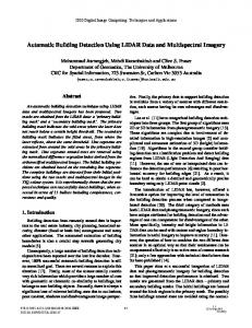
The work flow for our method for building extraction is depicted in fig. 1. The input to our method is given by three data sets that have to be generated from the raw data in a preprocessing step. The last pulse DSM is sampled into a regular grid by linear prediction using a straight line as the covariance function, so that the interpolation is carried out almost without filtering [8]. The first pulse DSM is also sampled into a regular grid. The normalised difference vegetation index (NDVI) is computed from the near infrared and a red band of the multispectral images we assume to be available [7]. These image data must be geocoded. We start by creating a DTM from the last pulse DSM by morphological grey scale opening using a square structural element. Initially, the size of the structural element corresponds to the size of the largest building available in the dataset. An initial building mask, basically a binary image of possible building pixels, is created mainly by thresholding operations. That building mask is morphologically opened to eliminate spurious and strangely shaped building areas, and then connected components of building pixels give an initial building regions. For these regions, we evaluate the surface roughness and the average NDVI. In the first iterations, very tight thresholds are applied to surface roughness, because we assume the largest buildings in the scene to consist of large planar surfaces. Thus, we obtain an intermediate set of building regions, only containing the largest and most salient buildings (corresponding to the current state of the DTM). After that, the whole procedure is repeated with a smaller structural element for morphological opening, but in the areas already classified as buildings, the DTM heights of the previous iteration are substituted for the results of the morphological filter. Thus, the buildings already detected are elim-
4
NDVI
DSM First Pulse
DSM Last Pulse Morphologic Filtering DTM
Thresholding of cues: height, size, NDVI, height differences first – last pulse Initial building regions Morphological operators, connected component analysis Evaluation of surface roughness and NDVI Building regions corresponding to current DTM Final Stage?
N
Y Final building regions
Fig. 1. The work flow for building detection.
inated, whereas the smaller size of structural element for morphological filtering helps to obtain a finer approximation for the DTM, rendering possible the separation of smaller buildings. The whole procedure is repeated with a decreasing size of the structural element until a user-specified minimum size is reached. The results of the final iteration are identical to the results of building detection, basically represented by a list of building regions and a building label image. In section 3, we will have a closer look at the individual processing stages.
3 3.1
Stages of Building Detection Morphological Filtering of the DSM
We assume the DSM to be a matrix containing the heights z(i, j), with integer matrix indices i and j. For morphological filtering of the DSM, a structural element W , i.e., a digital image w(m, n) representing a certain shape, has to be defined. Restricting ourselves to symmetrical structural elements having constant values, thus w(m, n) = w(−m, −n) and w(m, n) = 0 ∀[m, n] ∈ W , morphological opening is performed by first carrying out an morphological erosion, z=
min z(i − m, j − n)
(1)
[m,n]∈W
followed by a morphological dilation, z = max z(i − m, j − n) [m,n]∈W
(2)
5
yielding the morphologically opened height matrix z(i, j) [12]. The resulting height matrix does not contain objects smaller than the structural element W . If W is chosen to be greater than the largest building in the data set, all buildings are removed by morphological opening; however, if W is too large, terrain details might be removed, too. If W is chosen rather small, the results of morphological filtering will be closer to the original height matrix and, thus, to the terrain, but larger buildings will remain in the data set. This is the reason why we apply morphological filtering in the hierarchical framework described in section 2. 3.2
Generation of the Initial Building Label Image
Morphological filtering provides us with an approximation for the DTM. As described in section 2, for buildings aready detected, the DTM generated by morphological opening in the previous iteration is substituted for the results of morphological filtering, so that large buildings that would be preserved by morphological filtering in the current iteration are eliminated beforehand. An initial building mask is created by thresholding the height differences between the last pulse DSM and the DTM (e.g., by hmin =2.5 m). This initial building mask still contains spurious regions, areas covered by vegetation, and terrain structures smaller than the structural element for morphological filtering. In addition, individual buildings might not be separated correctly. At this instance, the additional data sources can be used to improve these results. First, a large NDVI indicates areas covered by vegetation, so that pixels having an NDVI above a certain threshold are erased in the building mask. Second, as pointed out in section 1.1, the heights from first and last pulse data will differ mainly in areas covered by trees and if the laser beam accidentally hits the roof edge of a building. Thus, in most cases, large height differences between first and last pulse data indicate trees. Pixels having a height differece larger than a certain threshold are erased in the building mask, too. A binary morphological opening filter using a structural element of a size corresponding to the expected minimum size of a building part (e.g., 3 × 3 m2 ) is applied to the initial building mask to erase oddly shaped objects such as fences and to separate building regions just bridged by a thin line of pixels. A connected component analysis of the resulting image is applied to obtain the initial building regions. Regions smaller than a minimum area are discarded. 3.3
Classification of Building Candidate Regions
Some of the initial building regions correspond to groups of trees or to terrain structures smaller than the structural element. These regions can be eliminated by evaluating a surface roughness criterion derived by an analysis of the second derivatives of the DSM. In [4], a method for polymorphic feature extraction is described which aims at a classification of texture as being homogeneous, linear, or point-like, by an analysis of the first derivatives of a digital image. The thresholds required for that classification are derived automatically from the image
6
data. This method is applied to the first derivatives of the DSM using an integration kernel of a size corresponding to, e.g., 5 m in object space. Under these circumstances, “homogeneous” pixels correspond to areas of locally parallel surface normal vectors, thus, they are situated in a locally planar neighbourhood. “Linear” pixels correspond to the intersections of planes. Finally, “point-like” pixels are in a neighbourhood of great, but anisotropic variations of the surface normal vectors. This is typical for building corners and for trees. For evaluating surface roughness, the numbers of “homogeneous” and “point-like” pixels are counted in each initial building region. Buildings are characterised by a large percentage of “homogeneous” and by a small percentage of “point-like” pixels. By comparing these percentages to thresholds, non-building regions can be eliminated. The surface roughness criterion works well for large buildings and with dense LIDAR data [8]. If the point distance of the LIDAR data is larger than, e.g., 1 m, only few LIDAR points will be situated on small buildings, so that the percentage of “homogeneous” pixels is reduced, whereas the percentage of “point-like” pixels is increased. Thus, it makes sense to additionally evaluate the average NDVI for each building region to eliminate vegetation areas. Finally, vegetation areas still connected to buildings are eliminated. By morphological opening, regions just connected by small bridges are separated. The resulting binary image is analyzed by a connected component analysis which results in a greater number of regions, and the terrain roughness criterion is evaluated again. Pixels being in regions now classified as containing vegetation are erased in the initial building label image. Thus, in vegetation areas originally connected to buildings, only the border pixels remain classified as “building pixels”. Again, morphological opening helps to erase these border pixels [8].
4 4.1
Experiments Description of the Data Set
The test data set was captured over Faifield (Victoria) using an Optech ALTM 3025 laser scanner. Both first and last pulse were recorded, the average point distance being about 1.2 m. We derived DSM grids at a resolution of 1 m from these data. Intensity data were available, too. We used an area of 2 × 2 km2 for our test. For that area, a true colour digital orthophoto with a resolution of 15 cm was available. The orthophoto was created using a DTM, so that the roofs and the tree-tops were slightly displaced with respect to the LIDAR data. Unfortunately, the digital orthophoto did not contain an infrared band. We circumvented this problem by resampling both the digital orthophoto and the (infrared) LIDAR intensity data to a resolution of 0.5 m and by computing a “pseudo-NDVI-image” from the LIDAR intensities and the green band of the digital orthophoto. Apart from problems with georeferencing caused by the displaced tree canopies in the orthophoto, there were also problems with shadow areas in the orthophoto, so that the “pseudo-NDVI-image” did not provide as valuable an information as the NDVI image was supposed to be. Still, it helped in classification. The input data for our test are shown in fig. 2.
7
Fig. 2. The Fairfield data set. Upper row, left: The DSM (black: low areas, white: high areas). Upper row, right: The colour orthophoto. There are industrial buildings in the northern central regions and residential houses in the west and south-west. Second row, left: The “pseudo-NDVI-image”. Second row, right: The height differences between first and last pulse data (black: large differences). Total area: 2000 × 2000 m2 .
4.2
Results
Fig. 3 shows the results of morphological opening of the DSM in fig. 2 using structural elements of two different sizes (150 m and 25 m). Using the large structural element, all buildings can be eliminated, but the terrain shape is not well preserved, so that the residential buildings in the lower part of the scene are merged. This can be seen in fig. 4, showing the initial building mask derived using the left DTM in fig. 3 (height threshold: 2 m). Using a smaller structural element, more terrain details are preserved, but the large buildings are still
8
Fig. 3. The results of morphological opening of the DSM using structural elements of 150 × 150 m2 (left) and 25 × 25 m2 (right).
contained in the data. However, using our hierarchic approach, these buildings can be eliminated beforehand, as described in section 2. The results of texture classification are presented in fig. 5 (filter kernel size: 3 × 3 pixels). Note the co-incidence of clusters of “point-like” pixels and vegetation areas such as those along the creek passing through the scene diagonally,
Fig. 4. The initial building mask corresponding to the left DTM in fig. 3. The residential buildings on a small hill at the southern border are merged.
Fig. 5. The classification results of polymorphic feature extraction. White: “homogeneous”, light grey: “linear”, black: “point-like”.
9
which is used to eliminate trees. In the first iteration, starting from the initial building mask in fig. 4, we only accept regions larger than 2500 m2 , containing less than 0.30% of “point-like” and at least 70% of “homogeneous” pixels, thus, large regions consisting of mostly planar roof planes. As the industrial buildings had a high reflectivity in the infrared part of the spectrum, the threshold for the “pseudo-NDVI” was kept at 75%. 85 mostly large building structures are detected in the first iteration (left part of fig. 6).
Fig. 6. Buildings extracted in the first (left) and third (right) iterations.
Altogether three iterations were carried out, using structural elements of 150 m, 75 m, and 25 m. In the final iteration, regions larger than 25 m2 , containing less than 85% of “pointlike” and at least 1% of “homogeneous” pixels were accepted. These relatively loose settings of the threshold were a consequence of the LIDAR resolution, with only few points and, thus, few “homogeneous” pixels on the roofs of the smaller buildings. 1589 buildings were detected (right part of fig. 6). The parameters for classification were chosen in a way to minimise the number of missed buildings, accepting a larger rate of false alarms. Less than Fig. 7. Boundary polygons super1% of the buildings were not detected. imposed to the orthophoto. Fig. 7 shows the orthophoto of a part of the test area super-imposed by the boundary polygons of the buildings. There remain some trees in the data, and some of the buildings are still merged, especially if the distance between them is small. However, as almost all the buildings are contained in the data, it might be possible to improve the results of classification by considering additional cues derived, for instance, from the colour images.
10
5
Conclusion and Future Work
We have presented a hierarchic method for building detection from LIDAR data and multispectral images, and we have shown its applicability in a test site of heterogeneous building shapes. In our test, we put more emphasis on detecting all buildings in the test data set than on reducing the false alarm rate because in the future we want this method to be the module for initial segmentation in a framework using more sophisticated methods of data fusion similar to those described in [7], replacing the rather heuristic methods used up to now. In order to further improve the segmentation results and to split building regions erroneously merged, the results of a segmentation of the orthophoto could be considered. Using the NDVI computed from real infrared images rather than the “pseudo-NDVI” used in this test might also help to improve the results.
Acknowledgements This work was supported by the Australian Research Council (ARC) under Discovery Project DP0344678. The Fairfield data set was provided by AAM Geoscan, Kangaroo Point, QLD 4169, Australia (www.aamgeoscan.com.au).
References 1. Brenner, C.: Dreidimensionale Geb¨ auderekonstruktion aus digitalen Oberfl¨ achenmodellen und Grundrissen. PhD Thesis, Institute of Photogrammetry, Stuttgart University, DGK-C 530 (2000). 2. Brunn, A., Weidner, U.: Extracting buildings from digital surface models. IAPRS XXXII(3-4W2) (1997) 27–34. 3. Briese, C., Pfeifer, N., Dorninger, P.: Applications of the robust interpolation for DTM determination. IAPSIS XXXIV/3A (2002) 55–61. 4. Fuchs, C.: Extraktion polymorpher Bildstrukturen und ihre topologische und geometrische Gruppierung. PhD Thesis, Institute of Photogrammetry, Bonn University, DGK-C 502 (1998). 5. Klein, L.: Sensor and Data Fusion. Concepts and Applications. SPIE Optical Engineering Press (1999). 6. Kraus, K.: Principles of airborne laser scanning. Journal of the Swedish Society for Photogrammetry and Remote Sensing 2002:1 (2002) 53–56. 7. Lu, Y. H. and Trinder, J.: Dempster-Shafer data fusion theory for automatic extraction buildings in 3D reconstruction. ASPRS Workshop Anchorage, Alaska (2003). 8. Rottensteiner, F. and Briese, C.: A new method for building extraction in urban areas from high-resolution LIDAR data. IAPSIS XXXIV/3A (2002) 295–301. 9. Schenk, T. and Csatho, B.: Fusion of LIDAR data and aerial imagery for a more complete surface description. IAPSIS XXXIV/3A (2002) 310–317 10. Vosselman, G., Dijkman, S.: 3D building model reconstruction from point clouds and ground plans. IAPSIS XXXIV(3W4) (2001) 37–43. 11. Vosselman, G.: On the estimation of planimetric offsets in laser altimetry data. IAPSIS XXXIV/3A (2002) 375–380. 12. Weidner, U.: Geb¨ audeerfassung aus digitalen Oberfl¨ achenmodellen. PhD Thesis, Institute of Photogrammetry, Bonn University, DGK-C 474 (1997).