Forth, I also want to thank my committee member, Dr. John Fowler, who is ...... back to 1986, when STABB (âShift to A Better Biasâ) is proposed by Utgoff (1986), ...
Building Energy Modeling: A Data-Driven Approach by Can Cui
A Dissertation Presented in Partial Fulfillment of the Requirements for the Degree Doctor of Philosophy
Approved April 2016 by the Graduate Supervisory Committee: Teresa Wu, Co-Chair Jeffery D. Weir, Co-Chair Jing Li John Fowler Mengqi Hu
ARIZONA STATE UNIVERSITY May 2016
ABSTRACT Buildings consume nearly 50% of the total energy in the United States, which drives the need to develop high-fidelity models for building energy systems. Extensive methods and techniques have been developed, studied, and applied to building energy simulation and forecasting, while most of work have focused on developing dedicated modeling approach for generic buildings. In this study, an integrated computationally efficient and high-fidelity building energy modeling framework is proposed, with the concentration on developing a generalized modeling approach for various types of buildings. First, a number of data-driven simulation models are reviewed and assessed on various types of computationally expensive simulation problems. Motivated by the conclusion that no model outperforms others if amortized over diverse problems, a metalearning based recommendation system for data-driven simulation modeling is proposed. To test the feasibility of the proposed framework on the building energy system, an extended application of the recommendation system for short-term building energy forecasting is deployed on various buildings. Finally, Kalman filter-based data fusion technique is incorporated into the building recommendation system for on-line energy forecasting. Data fusion enables model calibration to update the state estimation in realtime, which filters out the noise and renders more accurate energy forecast. The framework is composed of two modules: off-line model recommendation module and online model calibration module. Specifically, the off-line model recommendation module includes 6 widely used data-driven simulation models, which are ranked by meta-learning recommendation system for off-line energy modeling on a given building scenario. Only a selective set of building physical and operational characteristic features is needed to i
complete the recommendation task. The on-line calibration module effectively addresses system uncertainties, where data fusion on off-line model is applied based on system identification and Kalman filtering methods. The developed data-driven modeling framework is validated on various genres of buildings, and the experimental results demonstrate desired performance on building energy forecasting in terms of accuracy and computational efficiency. The framework could be easily implemented into building energy model predictive control (MPC), demand response (DR) analysis and real-time operation decision support systems.
ii
DEDICATION To my mom and dad, who have always been emotionally supportive.
iii
ACKNOWLEDGMENTS First, I would like to thank my advisor Dr. Teresa Wu for persevering with me throughout my study and research process for completing the degree. I sincerely appreciate her mentorship, guidance and cultivation, which makes my Ph.D. study one of the most valuable experiences in my life. Second, I would like to thank my co-advisor, Dr. Jeffery D. Weir, and my committee member, Dr. Mengqi Hu, who have always been generously given their time and expertise on my research through years. They have also offered me a great help on my paper writing and presentation skills. Third, I would like to thank my committee member, Dr. Jing Li, who has been supportive when I encountered difficulties in my research and guided me with valuable suggestions. Forth, I also want to thank my committee member, Dr. John Fowler, who is willing to step in and become my committee member given short notice. In addition, I have benefited greatly from his knowledge in the field of simulation. In addition, I’m grateful to my lab mates, who have shared their knowledge, expertise and experience with me and helped me with not only academic but also daily life problems. Finally, I must thank as well the department, friends, faculty, students, colleagues, and other staff who assisted, advised, and supported my research and writing efforts over the years.
iv
TABLE OF CONTENTS Page LIST OF TABLES ............................................................................................................ vii LIST OF FIGURES ........................................................................................................... ix CHAPTER 1
INTRODUCTION .................................................................................................. 1 Background ................................................................................................. 1 Literature Review........................................................................................ 2 Research Scope ......................................................................................... 13 Dissertation Organization ......................................................................... 18
2
A RECOMMENDATION SYSTEM FOR META-MODELING ON DATADRIVEN SIMULATIONS ................................................................................... 20 Introduction ............................................................................................... 21 Background ............................................................................................... 26 Proposed Framework ................................................................................ 39 Experiments and Results Analysis ............................................................ 47 Discussion and Conclusion ....................................................................... 57
3
SHORT-TERM BUILDING ENERGY MODEL RECOMMENDATION SYSTEM: A META-LEARNING APPROACH ................................................. 61 Introduction ............................................................................................... 62 Building Energy Model Recommendation System................................... 72 Experiments and Results ........................................................................... 83 v
CHAPTER
Page Discussion and Conclusion ....................................................................... 96
4
ON-LINE CALIBRATION OF DATA-DRIVEN MODELS FOR BUILDING ENERGY CONSUMPTION FORECASTING .................................................... 99 Introduction ............................................................................................. 100 Methodology ........................................................................................... 107 Experiments and Results ......................................................................... 116 Conclusions and Future Work ................................................................ 128
5
CONCLUSION AND FUTURE WORK ........................................................... 131 Summary ................................................................................................. 131 Conclusion and Future Work .................................................................. 132
6
REFERENCES ................................................................................................... 136
vi
LIST OF TABLES Table
Page
1. Summary on the Advantages and Disadvantages of the Three Types of Models 11 2. Performance Statistics of Meta-learners ............................................................... 52 3. Top Recommended Meta-model Given by Different Meta-learners (K-Kriging, SSVR, R-RBF, M-MARS, A-ANN, P-PR) ............................................................ 53 4. (Approximate) Computational Cost Comparison between the Traditional Trialand-Error Approach and Meta-learning Approach on each test problem ............. 54 5. Summary Statistics of Three Feature Selection Techniques: SVD, Stepwise Regression and ReliefF ......................................................................................... 57 6. Ten Selected Building Operational Features and two Categorical Variables ....... 75 7. Building Physical Features ................................................................................... 79 8. Test Case I: Statistics on Meta-learning SRCC, Success Rate and # of Successes across 48................................................................................................................ 88 9. Test case II: Statistics on Meta-learning SRCC, Success Rate and # of Successes across 48 Problems ............................................................................................... 91 10. Comparison between Ground Truth and Recommendation System on Mean of Best NRMSE across 48 Problems on Each Test Case .......................................... 92 11. Mean and Standard Deviation of the Computational Cost (in seconds) of the Six Models across 48 Problems .................................................................................. 93 12. Performance Rankings (T) of the Six Forecasting Models and the Predicted Rankings from BEMR (B) on Single Day and One Week Tests .......................... 95
vii
Table
Page
13. Ten Selected Building Operational Features and two Categorical Variables ..... 114 14. Performance of Each Recommended Model ...................................................... 119 15. Summary Statistics of the Distribution of Process Noise of the Baseline Model and the Corresponding SSM ............................................................................... 124 16. the Performance of Baseline, SSM and Kalman Filtering on Energy Consumption Forecast ............................................................................................................... 127 17. The Absolute Errors of Each Kalman Filtering Results ..................................... 128
viii
LIST OF FIGURES Figure
Page
1. Diagram of Concepts of Physics-based, Data-driven and Hybrid Model (http://energy.imm.dtu.dk/models/grey-box.html). .............................................. 10 2. Flowchart of Research Scope................................................................................ 18 3. A Schematic Diagram of Rice’s Model with Algorithm Selection Based on Features of the Problem. ....................................................................................... 37 4. A Pseudo Code of Meta-learning Based Recommendation System for Metamodeling. .............................................................................................................. 39 5. Uni-modal Function: Sphere Function.................................................................. 47 6. Multi-modal Function: Rotated Weierstrass Function. ......................................... 48 7. Composition Function: Composed of Three Multimodal Functions. ................... 48 8. Multiple Comparison Test on Mean NRMSE of Six Meta-models of Different Sample Sizes. ........................................................................................................ 51 9. Framework of Building Energy Model Recommendation (BEMR) System. ....... 72 10. “hv-block” Cross-validation Illustration. .............................................................. 77 11. Cross-validation of Training Data Split. ............................................................... 78 12. Test Case I: Bar Chart of Mean of Best NRMSE across 48 Problems on Each Test Case. ...................................................................................................................... 85 13. Weekly Cooling Electricity Load (Kwh) Time Series Plot of (a) Large Office in San Francisco, CA; (b) Large Office in Phoenix, AZ; (c) Full Service Restaurant in Phoenix, AZ. ..................................................................................................... 86 14. Test Case I: Bar Chart of Meta-learning Success Rate. ........................................ 87
Figure
Page
15. Test Case I: Bar Chart of Meta-learning SRCC.................................................... 87 16. Test case II: Bar Chart of Mean of Best NRMSE across 48 Problems on Each Test Case. ...................................................................................................................... 89 17. Box Plot of Mean of NRMSE on Test Cases I&II................................................ 90 18. Test case II: Bar Chart of Meta-learning Success Rate. ....................................... 91 19. Test case II: Bar Chart of Meta-learning SRCC. .................................................. 91 20. Energy Resource Station at Iowa Energy Center. ................................................ 94 21. Complete Kalman Filter Operations. .................................................................. 108 22. Workflow of the Proposed Framework of On-Line Forecast Model. ................. 112 23. One-day Ahead Forecast Comparison Plots with Different Measurement Noise. ............................................................................................................................. 120 24. Time Series Comparison Plot among ANN Simulation Model, the State Space Model (SSM) and the Real Data (10% noise). ................................................... 122 25. Simulation Error Time Series of ANN and SSM (10% noise). .......................... 124 26. Control Input to the SSM Model. ....................................................................... 125 27. Kalman Filter Energy Estimation of the Building. ............................................. 126 28. Comparison Plot Between KF Estimation of Energy Consumption and Real Energy Consumption. ......................................................................................... 126 29. Framework of Data-driven Building Energy Modeling...................................... 132
x
CHAPTER 1 INTRODUCTION 1.1 Background The U.S. Energy Information Administration (EIA) (Architecture 2030 2011) states that buildings consume nearly 50% of the total energy and around 30% of the consumption in buildings is used by heating, ventilating and air conditioning (HVAC) in the United States (Xiwang Li, Wen, and Bai 2016). Historical data shows, from 1996 to 2006, the electricity consumption of the US grows 1.7% annually, and the total growth will reach to 26% by 2030 (Parks 2009). This drives the need to develop high-fidelity energy models for building systems. Since the early 20th century, load simulation and forecasting has been a conventional and important activity in electric utilities across a number of applications, such as financial planning, operations and controls, and resource allocations, etc. Extensive methods and techniques have been developed, studied, and applied to load simulation and forecasting, while many challenging issues are still remaining unsolved. In terms of modeling design, how to achieve modeling accuracy and computational efficiency at the same time. In terms of model selection, how to select the appropriate models among a number of candidates. And in terms of modeling robustness, how to make the model adaptive to various uncertainties. We conclude there is a lack of systematic and integrated approach of building energy modeling framework. This chapter discusses the current practices in building load simulation and forecasting, introduces the fundamentals and classifications of building energy models, discusses the relations between forecasting and simulation, proposes a number of 1
research questions, and provides with an integrated energy modeling framework solution for performing building load forecasting tasks.
1.2 Literature Review As is known, there does not exist a universal forecast model that could satisfy all forecasting needs (T. Hong 2010). As a result, over the past decades, different types of building energy models have been developed for different purposes. Besides business needs, e.g., consumption analysis, control and operation optimization, pricing strategies, etc., the availability of the resources, e.g., weather forecast data, sensor data, economical information, etc., also affects the design and selection of forecasting model development. Based on the forecast horizon and updating cycle, the existing building energy forecasting could be categorized as short term load forecasting (STLF), medium term load forecasting (MTLF), and long term load forecasting (LTLF) (T. Hong 2010). STLF focuses on the load forecasting on daily basis and/or weekly basis, and MTLF and LTLF are based on monthly and yearly collected data for transmission and distribution (T&D) planning (H . Lee Willis 2004), and financial planning, which assist with medium to long term energy management, decision making on the utilities project and revenue management. STLF is important for real-time energy operations and maintenance. For daily operations, system operators can make switching and operational decisions, and schedule maintenance based on the patterns obtained during the load forecasting process (H. Wang et al. 2016). STLF is inherently connected to other types of forecasts by scaling and adjusting the parameters and elements in the model. Thus, it could be viably 2
transformed into MTLF or LTLF, by adding features, such as economics and land use, and extrapolating the model to longer horizons. To better assist the operations and control strategies development, this study mainly focuses on STLF approach, which provides the buildings with accurate load forecasts for daily and weekly based energy system management. The building energy simulation models could also be categorized as: “physicsbased” (white-box) models (Al-Homoud 2001; Katipamula and Lu 2006), “data-driven” (black-box) models (Ekici and Aksoy 2009; Aydinalp, Ugursal, and Fung 2004; Dong, Cao, and Lee 2005; Mihalakakou, Santamouris, and Tsangrassoulis 2002; Ozturk et al. 2004) and “hybrid” (grey-box) models (Q. Zhou et al. 2008; J. E. Braun and Chaturvedi 2002; Wen 2003). Extensive studies exist in the literature on these three types of building energy modeling approaches, which are closely reviewed in this Section.
1.2.1 Physics-based Models Physics-based (or white box) models are built based on detailed physical principles for modeling the building components, and sub-systems. It can make predictions on whole buildings and their sub-systems behaviors. They are known to be excellent dynamic models due to their detailed dynamic equations built from system physics. The set of numerous mathematical representations forms a simulation engine which simulates the building operation mechanisms and calculates the building energy consumption (Scotton et al. 2013). The number of parameters that need to be estimated in the physics-based model is typically large, because each and every detail of the 3
description of all the processes is involved in the system. Therefore, these types of simulation tools are usually elaborate and accurate. A number of white box software tools are available for both whole building and sub-system simulation, such as TRNSYS (Klein 2010) and EnergyPlus (Energy 2010). EnergyPlus is develop by Department of Energy of US and has been widely used as a whole building energy simulation tool for building energy research. It is known to be highly accurate simulation program used by engineers, architects, and researchers for modeling energy and water use in buildings. It allows the building professionals construct the building performance models on which optimization task could be conducted for design and operation strategies that render less energy and water usage. However, to build such elaborate system is not trivial task, which requires domain expertise on building architecture and thermal dynamic theories, involving with deep knowledge about detailed information and parameters of buildings, energy system and outside weather conditions. Moreover, to identify the modeling parameters takes long time and the simulation running process requires high-performance computing capability. The time-consuming model development and low-speed simulation process make it challenging to apply physics-based model on applications such as real-time energy consumption modeling and on-line model predictive control (MPC). As a result, the elaborate physics-based building energy models are more suitable for simulation purposes, where the objective is to estimate and observe the system response and behavior in a long-term time span.
4
1.2.2 Data-driven Model Data-driven models, also known as black box models, are defined as the models in which internal workings of the system are not described, but simply solves a numerical problem without reference to any underlying physics. This usually takes the form of a set of transfer parameters or empirical rules that relate the output of the model to a set of inputs. In simulation terminology, data-driven model is sometimes referred to as “metamodel”, “black box model” or “surrogate model”, which is a “model of the model” (J. P. Kleijnen 2008). Meta-model is often built when physics-based simulation is not computationally easily implemented. It simplifies the simulation in two ways: its response is determined by a set of simpler equations, and the run time is generally much shorter than the original simulation (Barton and Meckesheimer 2006). Therefore, metamodels are often used to approximate and replace the complex simulation models in computer-based engineering design and design optimization. Data-driven models could be categorized into statistical techniques, e.g., multivariate regression, and machine learning algorithms, e.g., Artificial Neural Network (ANN) (McCulloch and Pitts 1943). A comprehensive review of meta-modeling applications in engineering design is given by (T. W. Simpson et al. 2001). They review several of data-driven modeling techniques including design of experiments, response surface methodology, Taguchi methods, neural networks, inductive learning, and Kriging, and conclude with recommendations for the appropriate use of approximation techniques. Artificial neural networks consists of interconnected "neurons" which can train itself and make deduction from inputs. Support Vector Machine for regression 5
(SVR) (Clarke, Griebsch, & Simpson, 2005; Drucker, Chris, Kaufman, Smola, & Vapnik, 1997) is derived from support vector classification to find an optimal generalization of the training data set. A thorough review on popular data-driven models will be given in Chapter 2. Data-driven models are based on analyzing the data about a system, in particular finding connections between the system state variables (input, internal and output variables) without explicit knowledge of the physical behavior of the system. These methods represent advances on conventional empirical modelling and allow for solving numerical prediction problems, reconstructing highly nonlinear functions, performing classification, grouping of data and building rule-based systems (Solomatine and Ostfeld 2008). Data-driven modeling does not normally contain any physical knowledge regarding the system, and the physical parameters are partially hidden in the model parameterization. Therefore, data-driven modeling is desirable for short-term predictions. Black box models are useful when an answer to a specific problem is required while the flexibility to change aspects of a model and see the effect is not. The required flexibility of a model depends upon its long-term objectives as part of the design process. If the purpose of the model is only to provide quick, approximate answers, based on a predetermined set of input parameters, then a black box model is appropriate.
1.2.3 Hybrid Models A hybrid model, also known as “grey box” model, is built from partial theoretical structure and physical knowledge of the process combining with data to complete the 6
model (Bohlin 2006). To maintain the physical interpretation of the model, it would be suitable to use physical formulation and apply an estimation method, where the parameterization is obtained from data. The parameters in the model are physically interpretable and estimated by statistical methods. Grey box model is mixture of white and black model, since the basic model structure is inherited from the white box models, usually in the form of ordinary differential equations, but the parameter estimation and the uncertainty assessment are obtained using statistical methods. In a grey box model, certain elements within the model can be approximated by rules. The modeling development could be summarized as a three-step process: First, a simplified physics model for a system is developed as a foundation; Second, physical parameters are determined from the description of the system geometry and materials; Last, other model parameters are identified by user-defined algorithms from data. In building energy simulation, thermoelectricity analogy structure and lumped parameter models for energy devices are typical simplified physics based models (J. Braun and Chaturvedi 2002; Henze, Felsmann, and Knabe 2004). The model parameters are determined from the building systems properties and design factors, such as the energy device performance coefficient and thermal capacity of building envelope. Common methods for parameter determination include, such as, regression methods, optimization prediction error approach and maximum likelihood method, etc. For example, Resistance and Capacitance (RC) network model is one of the most common grey box models, which models building energy consumptions with a simplified physical representation for thermal flows in building. It can be used to predict the building heating and cooling load 7
(J. Braun and Chaturvedi 2002), as well as to estimate building temperatures (Oldewurtel et al. 2012; Lee and Braun 2008). Compared to white box model, it has less number of parameters to determine and compared to black box models, it requires less training data. However, determining the parameters of RC model still requires expertise on building internal design and structure, and knowledge on thermal dynamics, along with optimization and searching algorithms (S. Wang and Xu 2006).
1.2.4 Forecasting and Simulation It is worthwhile discussing about these two technical terminologies, forecasting and simulation, for clarification on their inner connections and differences. Forecasting is the process of predictions on the future based on past and present data and analysis of trends. For example, to predict weather conditions by extrapolating/interpolating previous data. Prediction is a similar, but more general term. Both forecasting and prediction might work on time series, cross-sectional or longitudinal data. Simulation is the imitation of the operation of a real-world process or system over time (Banks et al. 2004). The simulation model represents the key characteristics or behaviors/functions of the physical system or process. The model represents the system itself, whereas the simulation represents the operation of the system over time. Simulation allows one to accurately specify a system through the use of logically complex, and often non-algebraic, variables and constraints. It is widely used for modeling of human systems or natural systems for gaining insight into the functions (R. D. Smith and Chief Scientist 1999). Moreover, by simulation, it is possible to show the courses of actions and corresponding effects 8
provided alternative conditions of the systems. Simulation is also used when the real system cannot be engaged, because it may not be easily obtainable, or it is being designed but not yet realized, or it may simply does not exist (Sokolowski and Banks 2008). Forecasting and simulation are correlated, due to their inter-connected mechanisms and functionalities. Forecasting could be realized through simulations. For example, most of the weather forecasts use the information published by weather bureaus, which has their own complicated numeric computer simulation models to predict weather by taking many parameters into account. Therefore, simulation is an approach for realization of forecasting, while forecasting is an application of simulation. The main objective of this thesis is to develop high-fidelity models for forecasting building energy, thus, the models are generally referred to simulation models. Consequently, we focus on developing high-fidelity simulation models to be applied for forecasting purpose.
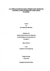
1.2.5 Summary We summarize the characteristics of physics-based, data-driven and hybrid models from different aspects including the model complexity, flexibility and accuracy and validity. It is then followed by our proposed modeling approach, combining with our business need and resource availability. The comparison diagram of physics-based model, data-driven model and hybrid model, developed by Madsen et al., is illustrated in Figure 1, which depicts the main components of the three models. 9
Physical knowledge
Prior Knowledge
Detailed subsystems
Data
Physics-based model
Hybrid model
Database
Input-Output relation Data-driven model
Figure 1 Diagram of Concepts of Physics-based, Data-driven and Hybrid Model (http://energy.imm.dtu.dk/models/grey-box.html).
As we discussed, it is important to choose the right type of model, based on the business need and available resources. Using the wrong type of model can result in failure of deliverables and waste of time and money. Therefore, the advantages and disadvantages of the three types of models are summarized in Table 1, which provides guideline on identifying model applicability.
10
Table 1 Summary on the Advantages and Disadvantages of the Three Types of Models Model Type
White box
Grey box
Black box
Advantages High flexibility: everything is modelled on a low level, so the behavior can be changed in line with the actual physics; Closeness to reality: provides the closest match to the real device.
Moderate flexibility; Closeness to reality: Partially built based on physics, and provides robust and accurate predictions under different operating conditions.
Low complexity: consists of a set of rules and equations that are easy to evaluate and can run very rapidly; Minimal required manpower and computing power.
Disadvantages High complexity: contains no or few approximations, resulting in most complex model; High manpower: Requires domain expertise; High computing overheads: requires fast computers and large amounts of memory. Moderate complexity: both physics and data are required to estimate the model; Moderate manpower and computing overhead: Requires building information and domain expertise. Lack of flexibility: bounded to the training building operating conditions; Interpretation ability: lack of any form of physical meanings.
Examples
EnergyPlus simulation model
Resistance and Capacitance (RC) model
Artificial Neural Network
From Table 1, it can be concluded that different types of models have different properties and thus different applicability. The two major researching objectives of recent studies on building simulation modeling are increasing simulation speed and maintaining simulation accuracy (Xiwang Li and Wen 2014a). Therefore, the research objective of this study is to develop an integrated computationally efficient and high-fidelity building energy modeling framework, which could provide real-time accurate fast approximations 11
of the building energy systems with high degree of adaptivity and minimum computing efforts. The developed model could be cheaply implemented into building energy operation optimization, sensitivity analysis, what-if analysis and real-time engineering decisions. Moreover, in choosing the appropriate modeling approach, we also consider the following requirements: 1) Forecasting horizon: The model should be designed to assist in short term modeling (hourly based or daily based). In order to adapt the developed model with real time building operation and decision controls, a fast and real-time evaluation of the system is required. 2) Required level of flexibility: The model needs not to be highly flexible, because our research scope focuses on real-time building energy modeling, in facilitating the building operation and control design optimization. The update cycle granularity is generally within hourly-basis or daily basis. As a result, the design operation bounds are usually covered by the training data. A quick and accurate approximation model is preferable than a cumbersome time-consuming model. 3) The resource availability: Sometimes, the selection of the type of model is limited by the available computing power and manpower. Domain experts’ knowledge is needed to build detailed white box model, which is not always available. In such a case, a simplified model is needed. Based on the above considerations, in this research, we mainly focus on datadriven modeling approach for the building energy model development. Several key issues are involved with data-driven simulation modeling, such as selection of key 12
characteristics about the relevant system behaviors, acquisition of valid resource information, the assumptions within the simulation and the use of simplifying approximations, and fidelity and validity of the simulation outcomes. We summarize our research questions as follows:
The choice of the modeling functional form, i.e., the assumptions within the simulation and the use of simplifying approximations;
The choice of modeling inputs, i.e., key characteristics about the system behaviors;
Data acquisition and data reliability, i.e., acquisition of valid resource information;
Computational efficiency of the model;
The design of experiments: sampling strategy, parameter tuning, validation method, etc.;
Model adaptivity to uncertainties and generalizability to different building scenarios;
Assessment of the adequacy of the fitted model, i.e., fidelity and validity of the simulation outcomes;
These research questions are elaborately discussed and addressed in Chapter 2, 3 and 4.
1.3 Research Scope The overall research objective is to develop an integrated computationally efficient and high-fidelity building energy modeling framework with high degree of adaptivity and generalizability and minimum computing efforts. To fulfill this objective, we set our modeling targets to various building scenarios, rather than some specific building types. We argue that a single simulation modeling assumption may not be 13
adequate for serving the purpose of modeling various types of building energy systems. Therefore, a number of data-driven simulation models are first reviewed and assessed on various types of “black-box” problems. Motivated by the conclusion that no model outperforms others if amortized over diverse types of problems (Cui et al. 2014), we propose an integrated recommendation system for data-driven model selection on the cross-sectional data, which are depicted by various features derived from the design space. To test the feasibility of the proposed framework on the building energy system, we further extend the application of the recommendation system for forecasting on various building energy time series data using the same set of data-driven models. Finally, Kalman filter-based data fusion technique is incorporated into the building recommendation system for on-line energy forecasting. The proposed building energy simulation and forecasting framework is desired to be an integrated, intelligent and adaptive system, where human involvement is lessened, computational efficiency is improved and automatic decision making on model selection is realized. The research topics and proposed solutions associated with the following Chapters along with a brief summary is given below. Research Topic 1: What are the most appropriate data-driven models for a given simulation problem? Proposed Solution: We propose a meta-learning based recommendation system for metamodeling on cross-sectional data. We first evaluate different meta-models on various black-box problems, and find that the performance of each model depends on the problems studied. Therefore, we 14
propose a general framework of a meta-model recommendation system by applying meta-learning technique for computationally expensive simulation tasks. 44 benchmark problems are tested using the proposed framework which includes uni-modal, multimodal and composition functions. Not only traditional statistical features, but also novel geometrical features are developed for problem characterization. Two types of metalearning algorithms, instance-based learning and model-based learning, are implemented and compared based on two evaluation criteria, Spearman’s ranking correlation coefficient and hit ratio. In addition, feature reduction techniques, including Singular Value Decomposition, Stepwise Regression and ReliefF, are applied on the feature space to further improve the meta-learning performance. The experiments show that the proposed framework is efficient and effective in making recommendation on metamodels for any given simulation problem. Research Topic 2: What are the most appropriate forecasting models on energy consumption forecasting for a specific building? Proposed Solution: We propose a meta-learning based recommendation system for building energy forecasting using data-driven models. Continued from the study on cross-sectional data, we want to further explore the applicability of the recommendation system to the building energy time series data. Therefore, we propose a framework of forecasting model recommendation system by applying the meta-learning technique on various computationally expensive building simulations. 48 benchmark building simulation models are tested using the proposed framework. In addition, a careful design of experiments on the modeling process is 15
elaborated, including feature engineering on building variables, training data selection and cross-validation on time series data. The meta-features are derived not only from the building electricity load time series, but also from the building design and operational variables and building physical description variables, in order for comprehensive characterization on various building scenarios. Based on the first study, a model-based meta-learning algorithm, specifically, an artificial neural network, is applied to model the relationship between the meta-features and the ranking derived from the meta-models’ performance. In addition, due to high dimensionality of the proposed meta-feature space, advanced feature reduction technique, Singular Value Decomposition, which is concluded to be efficient and effective in the first study, is applied on the meta-feature space to improve the meta-learning performance and reduce computational cost. The resulting high hit ratio (90%) indicates the successful implementation of the recommendation system on forecasting models for various building scenarios. Research Topic 3: How to develop on-line data fusion for data-driven model calibration with system uncertainties? Proposed Solution: We propose to develop an on-line data fusion system based on system identification and Kalman filter for calibrating the recommended model. Buildings are dynamical systems with noisy conditions and stochastic physical and occupancy characteristics. The fidelity of the static model may deteriorate as the system is continuously affected by outside disturbance and sensor noise. Therefore, online calibration using data fusion techniques are needed for improving the accuracy. To address this issue, sequential on-line data fusion for building energy model calibration is 16
a viable approach and in building research and practice, the Kalman filter is the most commonly used method. However, Kalman filter requires state space form of the system for state estimation. We propose to implement subspace-based system identification method, specifically, canonical variate analysis (CVA) for identifying the parameters of the given model as a state space representation upon which Kalman filtering can be applied. As a result, we propose a three-stage generalized framework for online calibration of data-driven models which may be state-space free. In the first stage, an appropriate data-driven model is recommended by the building model recommendation system developed in the previous research for off-line energy modeling. In the second stage, CVA is applied to transform the off-line model into a state space representation. In the third stage, Kalman filter is applied for on-line model calibration by real-time data fusion of the measurements. The proposed forecast model is tested on the energy consumption data of a commercial building simulation model, where three levels, small, medium and large of Gaussian noises are added to the system as measurement noises. The experimental results show that the proposed Kalman filtering data fusion model significantly improves the forecasting accuracy on average of 22%. In summary, the research scope of this dissertation is given in Figure 2. The IIIphase research steps provide with a comprehensive and integrated system methodology for high-fidelity, efficient and intelligent building energy forecasting.
17
Phase I: Recommendation system of metamodels for blackbox simulations problems
Phase II: Recommendation system of forecasting models for building energy time series data
Phase III: On-line calibration of data-driven models for building energy forecasting
Figure 2 Flowchart of Research Scope.
1.4 Dissertation Organization The rest of this dissertation is organized into three interrelated chapters that address building energy forecasting model selection and calibration, followed by the conclusion Chapter 5. Chapter 2 discusses the proposed meta-learning based recommendation system for meta-modeling on cross-sectional data. 44 black-box benchmark problems are tested using the proposed framework. Two types of metalearning algorithms, instance-based learning and model-based learning, are implemented and compared based on two evaluation criteria, Spearman’s ranking correlation coefficient and hit ratio. Advanced feature reduction techniques are applied on the feature space to further improve the meta-learning performance. Furthermore, encouraged by the promising result obtained from Chapter 2, we implement the recommendation system using meta-learning approach on the building energy forecasting problems in Chapter 3. 48 benchmark building simulation models are tested using the proposed framework of forecasting model recommendation system. Various meta-features are derived from multiple data sources. An artificial neural network is applied to model the relationship between the meta-features and the ranking derived from the meta-models’ performance. 18
In addition, advanced feature reduction technique, Singular Value Decomposition, which is concluded to be efficient and effective in Chapter 2, is applied on the meta-feature space to improve the meta-learning performance and reduce computational cost. Finally, in Chapter 4, we implement on-line data fusion to further calibrate the recommended forecast model, which could be derived from Chapter 3. Subspace-based system identification method is adopted to identify the parameters of the given data-driven simulation model as a state space representation upon which Kalman filtering can be applied. The proposed data fusion framework is tested on the consumption data of a commercial building simulation model. Chapter 5 summarizes the dissertation with conclusion remarks and discussions on future work.
19
CHAPTER 2 A RECOMMENDATION SYSTEM FOR META-MODELING ON DATA-DRIVEN SIMULATIONS Various meta-modeling techniques have been developed to replace computationally expensive simulation models. The performance of these meta-modeling techniques on different models are varied which makes existing model selection/recommendation approaches (e.g., trial-and-error, ensemble) problematic. To address these research gaps, we propose a general meta-modeling recommendation system using meta-learning which can automate the meta-modeling recommendation process by intelligently adapting the learning bias to problem characterizations. The proposed intelligent recommendation system includes four modules: 1) problem module, 2) meta-feature module which includes a comprehensive set of meta-features to characterize the geometrical properties of problems, 3) meta-learner module which compares the performance of instance-based and model-based learning approaches for optimal framework design, and 4) performance evaluation module which introduces two criteria, Spearman’s ranking correlation coefficient and hit ratio, to evaluate the system on the accuracy of model ranking prediction and the precision of the best model recommendation, respectively. To further improve the performance of meta-learning for meta-modeling recommendation, different types of feature reduction techniques, including singular value decomposition, stepwise regression and ReliefF, are studied. Experiments show that our proposed framework is able to achieve 94% correlation on model rankings, and a 91% hit ratio on best model recommendation. Moreover, the 20
computational cost of meta-modeling recommendation is significantly reduced from an order of minutes to seconds compared to traditional trial-and-error and ensemble process. The proposed framework can significantly advance the research in meta-modeling recommendation, and can be applied for data-driven system modeling.
2.1 Introduction The growing complexity of real-world systems drives research to develop simulation models to imitate the underlying functionality of the actual system (Banks et al. 2004). In general, the models can be categorized into three groups: physics-based modeling, data-driven modeling and a hybrid of the two. Physics-based models simulate the behavior of a real system based on the fundamental physics of each component and the interactions of the components, thus it can provide a high-fidelity description of the systems. However, the development of such models requires domain expertise for setting up and implementation. In addition, it suffers from high computational cost. A hybrid model is built upon the physics-based model using statistical tools to estimate the model parameters (Kristensen, Madsen, and Jørgensen 2004). It again, requires partial knowledge of the underlying system as a prior, which may not be easily obtained. Recently, the data-driven modeling approach has emerged as an alternative to model the system purely from the data available. A data-driven model, also known as a meta-model or surrogate model, is a “model of the model” (J. P. C. Kleijnen 1995). It is constructed using data which can provide fast approximations of the objects and has been used for
21
design optimization, design space exploration, sensitivity analysis, what-if analysis and real-time engineering decisions. Extensive research has explored a number of meta-models, e.g., Kriging (Matheron 1960), support vector regression (SVR) (Clarke, Griebsch, & Simpson, 2005; Drucker, Chris, Kaufman, Smola, & Vapnik, 1997), radial basis function (RBF) (Dyn, Levin, and Rippa 1986), multivariate adaptive regression splines (MARS) (Friedman 1991), artificial neural network (ANN) (McCulloch and Pitts 1943) and polynomial regression (PR) (Gergonne 1974), just to name a few. A comprehensive review of the meta-modeling applications in computer-based engineering design and optimization can be found in (Simpson, Peplinski, Koch, & Allen, 1997; Wang & Shan, 2007). As expected, the general conclusion from these studies is that the performances of the metamodels vary depending on the problems investigated. This is also confirmed by (Clarke, Griebsch, and Simpson 2005) and (Cui et al. 2014). Therefore, researchers have taken a trial-and-error approach, that is, investigating a number of different meta-models among which the best performer (evaluated against metrics, e.g., accuracy) is selected. It is not until recently that research started to explore the use of an ensemble, an optimal combination of several models. The distinct challenge these approaches (trail-and-error and ensemble) face is the expensive computational costs. Taking a large-scale metamodel based design optimization problem as an example, where thousands or even millions of fitness evaluations are triggered in support of the optimization process, building several meta-models or an ensemble might be computationally unaffordable.
22
In this research, we propose a meta-model recommendation system using a metalearning technique to identify the appropriate meta-models for engineering simulation problems which are known to be computationally expensive. Please note meta-learning is not new, it has been studied in machine learning fields, e.g., gene expression classification (Souza, Carvalho, and Soares 2008), failure prediction (Lan et al. 2010), gold market forecasting (Zhou, Lai, & Yen, 2012) and recommendation of classification algorithms on educational datasets (Romero, Olmo, and Ventura 2013). The idea of metalearning is that the information gained from learned instances shall be valuable to study future instances. To the best of our knowledge, most existing meta-learning systems handle the learning process on instances with a large volume of data records provided. As a result, the overall underlying structure of the instances can be well captured by the features extracted from the dataset. In this research, we are motivated to develop metamodel recommendation expert system for simulation purpose. Therefore, several unique challenges arise:
How to intelligently select sample data for meta-modeling?
In identifying the exemplar meta-model for a specific new problem, researchers have proposed instance-based (e.g., k-nearest-neighbors) vs. model-based (e.g., artificial neural network) meta-learning algorithms. To develop a meta-learning based metamodeling recommendation for simulation, which approach is appropriate?
Given the dataset, existing research tends to collect as many meta-features as possible which may lead to a large yet redundant set of meta-features. Which feature reduction technique is appropriate to reduce the dimensionality of the meta-features? 23
To answer these questions, our proposed recommendation system is designed with four modules: the problem space with an intelligent sampling module, a metafeature space module, an algorithm space module, and a performance space module. The problem space module is the repository of the problems being studied; intelligent sampling is launched to identify the representative dataset. The problem space is to be updated accordingly as new problems emerge. From the derived dataset, the meta-level features describing the characteristics of the problems/datasets are to be captured. Dimension reduction techniques, which include singular value decomposition (SVD) (Fallucchi, Zanzotto, & Rome, 2009; Simek et al., 2004), stepwise regression (Draper & Smith, 1981; Efroymson, 1960; Hocking, 1976) and the ReliefF method (Kira & Rendell, 1992; Kononenko, Šimec, & Robnik-Šikonja, 1997) may be applied to process the high dimensional meta-features. The algorithm space module consists of the meta-models to be chosen from and the performance space provides the metric(s) on which the metamodel is evaluated (multiple metrics may apply depending on the problem scope). To test the applicability of the proposed recommendation system: (1) 44 benchmark functions with distinct characteristics and properties, are collected from IEEE CEC 2013&2014 (Liang & Qu, & Suganthan, 2013a, 2013b); (2) Latin hypercube sampling is applied for the generation of a representative dataset for each problem; (3) 15 meta-features (statistical and geometrical) are derived from the generated dataset, and three feature reduction methods (SVD, stepwise regression, ReliefF) are then applied to reduce the dimensionality of the features, respectively; (4) Six meta-models are of interest including Kriging, SVR, RBF, MARS, ANN and PR; (5) Two types of meta-learning algorithms 24
(instance-based and model-based) are applied and compared, for exploration on appropriate designs; (6) Normalized root mean square error (NRMSE) is used as the accuracy measurement of each meta-model studied in the algorithm space module; (7) The performance of the proposed meta-learning framework is first assessed using the Spearman’s ranking correlation coefficient (Brazdil, Soares, & Costa, 2003; de Souto et al., 2008), a nonparametric measure of statistical dependence between derived rankings and ideal rankings. A second assessment metric, hit ratio, is introduced which is defined as the percentage of matches between the recommended best performer to the true best performer. Experiments show that our proposed framework is able to achieve 94% correlation on rankings, and a 91% hit ratio on best performer recommendation (40 out of 44 problems). In summary, the contributions of the proposed recommendation system are fourfold: 1) To the best our knowledge, this may be the first attempt to apply meta-learning on meta-modeling for automating the surrogate modeling process on computationally expensive simulation tasks. 2) The proposed generalized meta-model recommendation framework can significantly reduce the computational cost in the traditional trial-anderror or ensemble modeling process. 3) A comprehensive set of meta-features is proposed to characterize the properties of various black box problems. Different types of feature reduction techniques, including singular value decomposition, stepwise regression and ReliefF are studied to improve the recommendation system performance. 4) The proposed recommendation system is validated on a large number of benchmark cases, which is shown to be able to significantly improve the meta-modeling process, both on 25
the efficiency of model construction and the quality of the meta-model selection. The resulting intelligent expert system can benefit extensive research applications where automatic model selection is desired. This Chapter is organized as follows: Section 2.2 reviews background of metamodeling and meta-learning; In Section 2.3, the proposed methodology is elaborated; Section 2.4 describes the design of experiments and discusses results obtained; Finally, Section 2.5 draws the conclusions.
2.2 Background This section gives a general review on meta-modeling and meta-learning. “Meta”, meaning an abstraction from a concept is used to complete or add to that concept. Metamodeling refers to the modeling of a model, while meta-learning refers to the learning of the learning process. As a matter of fact, both deal with meta-level learning, while in different domains.
2.2.1 Meta-modeling The meta-modeling process involves model fitting or function approximation to the sampled data of design variables and responses from the detailed model (Ryberg, Bäckryd, and Nilsson 2012). To demonstrate the idea of our proposed framework, one parametric technique (PR), and five non-parametric techniques (Kriging, SVR, RBF, MARS and ANN) are chosen due to their extensive use in meta-modeling. Each is reviewed in the following section. For parametric techniques, a chosen functional 26
relationship between the design variables and the response is presumed. While nonparametric techniques, also known as distribution free methods, rely less on a priori knowledge about the form of the true function but mainly on the sample data for function construction.
2.2.1.1 Kriging Kriging (also known as Gaussian process regression) is an interpolation method that assumes the simulation output may be modeled by a Gaussian process. It gives the best linear unbiased prediction of simulation output not yet observed. It generates the prediction in the form of a combination of a global model with local random noise: 𝑦(𝑥) = 𝑓(𝑥)𝛽 + 𝑍(𝑥),
(1)
where x is the input vector, 𝛽 is the weight vector, and Z(x) is a stochastic process with zero mean and stationary covariance of 𝐶𝑂𝑉[𝑍(𝑥𝑖 ), 𝑍(𝑥𝑗 )] = 𝜎 2 𝑅(𝑥𝑖 , 𝑥𝑗 ),
(2)
where 𝜎 2 is the process variance, 𝑅(𝑥𝑖 , 𝑥𝑗 ) is an n by n correlation matrix where n is the sample size of the training data. R is usually depicted by a Gaussian correlation function, 𝑒𝑥𝑝(−𝜃(𝑥𝑖 − 𝑥𝑗 )2 ) with parameter 𝜃. Kriging is one of the most intensively studied meta-models because it is flexible with a number of correlation functions and regression functions (with polynomial degree of 0, 1 or 2) to choose from. It is generally acknowledged that the Kriging model outperforms others on nonlinear problems. However, it is also noted that it is time consuming to implement Maximum Likelihood 27
Estimation of the correlation parameters in R, which is a multi-dimensional optimization problem (Jin, Chen, and Simpson 2001).
2.2.1.2 Support Vector Regression Support Vector Regression (SVR) is analogous to support vector classification, which attempts to maximize the distance between two classes of data by selecting two hyperplanes to optimally separate the training data. The mathematical form of SVR is: 𝑓(𝑥) = 〈𝜔 ∙ 𝑥〉 + 𝑏,
(3)
where 𝜔 is the norm vector to the hyperplane and 𝑏/‖𝜔‖ determines the offset of the hyperplane from the origin. The goal is to find a hyperplane that separates the data points optimally without error and separates the closest points with the hyperplane as far as possible. Thus, it can be constructed as an optimization problem: min 1/2|𝜔|2 𝑦 − 〈𝜔 ∙ 𝑥𝑖 〉 − 𝑏 ≤ 𝜀 s.t. { 𝑖 . 〈𝜔 ∙ 𝑥𝑖 〉 + 𝑏 − 𝑦𝑖 ≤ 𝜀
(4)
According to the duality principle, the nonlinear regression problem is given by: ∗ 𝑓(𝑥) = ∑𝑚 𝑖=1(𝛼𝑖 − 𝛼𝑖 ) 𝑘〈𝑥𝑖 ∙ 𝑥𝑗 〉 + 𝑏,
(5)
where 𝛼𝑖∗ and 𝛼𝑖 are two introduced dual variables, and 𝑘〈𝑥𝑖 ∙ 𝑥𝑗 〉 is a kernel function, e.g. Gaussian kernel. It is noted that there exists research demonstrating the outperformances of SVR (G. G. Wang and Shan 2007), yet, most so far have been empirical studies.
28
2.2.1.3 Radial Basis Function Radial Basis Function (RBF) is used to develop interpolation on scattered multivariate data. A RBF is a linear combination of a real-valued radially symmetric function, ∅(𝑥), based on distance from the origin, 𝑓(𝑥) = ∑𝑛𝑖=1 𝜃𝑖 ∅(‖𝑥 − 𝑥𝑖 ‖),
(6)
where 𝜃𝑖 is the unknown interpolation coefficient determined by the least-squares method, n is the number of sampling points and ‖𝑥 − 𝑥𝑖 ‖ is the Euclidean norm of the radial distance from design point 𝑥 to the sampling point 𝑥𝑖 . Fang, Rais-Rohani, Liu, and Horstemeyer (2005) found RBF performs well on highly nonlinear problems.
2.2.1.4 Multivariate Adaptive Regression Splines Multivariate Adaptive Regression Splines (MARS) is a form of regression analysis introduced by Friedman (1991). A set of basis functions, defined as constant, hinge function, or the product of two or more hinge functions, are combined in the weighted sum form, as the approximation of the response function. A MARS model is built with generalized cross validation regularization in a forward/backward iterative process. The general model of MARS can be written as: 𝑓(𝑥) = 𝛾0 + ∑𝑚 𝑖=1 𝛾𝑖 ℎ𝑖 (𝑥),
(7)
where 𝛾𝑖 is the constant coefficient of the combination whose value is jointly adjusted to give the best fit to the data, and the basis function ℎ𝑖 , can be represented as: 𝐾
𝑚 ℎ𝑖 (𝑥) = ∏𝑘=1 [𝑠𝑘,𝑚· (𝑥𝑣(𝑘,𝑚) − 𝑡𝑘,𝑚 )]𝑞+ ,
29
(8)
where 𝐾𝑚 is the number of splits given to the mth basis function, 𝑠𝑘,𝑚 =±1 indicates the right/left sense of the associated step function, 𝑣(𝑘, 𝑚) is the label of the variable, and 𝑡𝑘,𝑚 represents values (knot locations) of the corresponding variables. The superscript q and subscript + indicate the truncated power functions with polynomials of lower order than q. According to (Jin, Chen, and Simpson 2001), MARS procedure appears to be accurate due to its distribution free assumption compared to other algorithms.
2.2.1.5 Artificial Neural Network Artificial Neural Network (ANN) (Rosenblatt 1958) is a computational model inspired by an animal's central nervous system. It is apt at solving problems with complicated structures. Due to its promising results in numerous fields, ANN has been extensively applied in stochastic simulation meta-modeling (Fonseca, Navaresse, & Moynihan, 2003; Nasereddin & Mollaghasemi, 1999). An ANN model typically consists of three separate layers: the input layer, the hidden layer(s), and the output layer. The neurons across different layers are interconnected to transmit and deduce information. A typical ANN with three layers and one single output neuron has the following mathematical form: 𝑓(𝑥) = ∑𝐽𝑗=1 𝜔𝑗 𝛿(∑𝐼𝑖=1 𝑤𝑖𝑗 𝛿(𝑥𝑖 ) + 𝛼𝑗 ) + 𝛽 + 𝜀
(9)
where 𝑥 is a k-dimensional vector, the input unit represents the raw information that is fed into the network, 𝛿(∙) is the user defined transfer function, 𝑤𝑖𝑗 is the weight factor on the connection between the ith input neuron and the jth hidden neuron, 𝛼𝑗 is the bias in the 30
jth hidden neuron, 𝜔𝑗 is the weight on connection between the jth hidden neuron and the output neuron, 𝛽 is the bias of the output neuron, ε is a random error with a mean of 0, and I and J are the number of input neurons and hidden neurons. In supervised learning, the output unit is trained to simulate the underlying structure of the input signals and response. The trained structure is depicted by several parameters, the weights on each connection, the biases, the number of hidden layers, the transfer functions, and the number of hidden nodes in each hidden layer. It is worth mentioning that the performance of ANN is highly dependent on parameter tuning, and extensive research have been done on this regard (Bashiri & Farshbaf Geranmayeh, 2011; Packianather, Drake, & Rowlands, 2000).
2.2.1.6 Polynomial Regression Polynomial Regression (PR) is a variation of linear regression in which a nth order polynomial is modeled to formulate the relationship between the independent variable x and the dependent variable y. PR models have been applied to various engineering domains such as mechanical, medical and industrial (Barker et al., 2001; Greenland, 1995; Shaw et al., 2006). A second-order polynomial model can be expressed as: 𝑓(𝑥) = 𝛽0 + ∑𝑘𝑖=1 𝛽𝑖 𝑥𝑖 + ∑𝑘𝑖=1 𝛽𝑖𝑖 𝑥𝑖 2 + ∑𝑖 ∑𝑗 𝛽𝑖𝑗 𝑥𝑖 𝑥𝑗 + 𝜖
(10)
where 𝛽 is the constant coefficient, 𝑘 is the number of variables, and 𝜖 is an unobserved random error with zero mean. PR models are usually fit using the least squares method. One advantage of PR models is the straightforward hierarchical structure, where the 31
significances of different design variables are directly reflected by the magnitude of the coefficients in the model. This is especially useful when the design dimension is large, where only significant factors are kept in the model and thus reduce the possibility of over-fitting. However, when fitting on highly nonlinear behaviors, PR may suffer from numerical instabilities (Barton 1992).
2.2.1.7 Summary Wolpert (1996) showed that bias-free learning is futile. In fact, researchers have claimed that a learning process without any prior knowledge about the system’s nature may lead to random solutions. As a result, existing research concluded the performance of meta-models is problem dependent, which confirms the classical No Free Lunch Theorem (NFL) (D.H. Wolpert and Macready 1997), that is, no algorithm can outperform any other algorithm when performance is amortized over all functions. Therefore, traditional approaches take a trial-and-error manner where a number of different metamodels are separately built and the best one is finally chosen. A comparison study on polynomial, Kriging, RBF, and MARS meta-models was conducted by Clarke, Griebsch, & Simpson (2005), which concluded that SVR generally outperforms others on accuracy and robustness. In a separate study (Cui, Wu, Hu, Weir, & Chu 2014), in which Kriging, SVR and RBF were compared in terms of accuracy and robustness, it was found that Kriging overall performs the best. The discrepancy on the conclusions between the two studies shows that the meta-modeling performance not only depends on the test problems, but also is compounded by the design of experiments and the model parameter 32
settings. A Gaussian process meta-model was used as the surrogate model for the timeconsuming finite-element model on a simple flat steel plate and a full-scale arch bridge in (Wan and Ren 2015). The authors favored a Gaussian process meta-model because of its probabilistic, nonparametric features and high capability of modeling a complex physical system. However, Gaussian process is not the only one that bears these merits, e.g., ANN is also nonparametric and is of powerful capability on complex system modeling. The selection of a single meta-model is very risky in the sense that researchers may end up with a sub-optimal model solution given no justification on other models’ inappropriateness. Therefore, traditional research has also explored the application of ensemble (Acar 2015), the combination of several models, which takes advantage of each meta-model’s strength and mitigate the weakness, thus result in stronger than any standalone meta-model. A multi-objective design optimization using dynamic ensemble metamodeling method was conducted to seek the optimal designs of a proposed functionally graded foam-filled tapered tube in (Yin et al. 2014). The authors claimed that the ensemble metamodeling method performs better than a single static meta-model. However, as the ensemble is built by four different meta-models, including Kriging, SVR, RBF, and PR, the computational cost is much higher than building a single model, which was not addressed in this work. In effect, for large-scale problems, e.g., metamodel based design optimization, in which thousands of fitness evaluations are called in support of the optimization process, building several meta-models or ensemble for each evaluation might be impractical. To summarize, two approaches are mainly involved with traditional meta-modeling research: (1) subjectively select a single meta-model for the 33
given surrogate modeling tasks, regardless of applicability and adaptability; (2) Ensemble on several meta-models, but at the expense of higher computational cost. Therefore, there is a need of a meta-learning approach to effectively associating the algorithm performance with the problem.
2.2.2 Meta-Learning Meta-learning is a machine learning approach to explore the learning process and understand the mechanism of the process, which could be re-used for future learning. Compared to base-learning, which learns a specific task (e.g., credit rating, fraud detection, etc.) on the corresponding data, meta-learning is a learning process that continuously gains knowledge as tasks being accomplished by the base-learners accumulate. The main goal is to build a flexible automatic learning machine that can solve different kinds of learning problems by using meta-data such as, the learning algorithm properties, the characteristics of the learning problems, or patterns previously derived from the relationship between learning problems and the effectiveness of different learning algorithms, and hence to improve the performance of the learning algorithms. For a comprehensive review of meta-learning research and its applications, we refer the reader to (Giraud-Carrier 2008; P Brazdil et al. 2008; Vilalta and Drissi 2002). Here we provide a general overview of a meta-learning framework followed by a review of its application to regression algorithm selection/recommendation which is of interest in this research.
34
2.2.2.1 Meta-Learning – Rice’s Model The early contribution related to computer programming on meta-learning dates back to 1986, when STABB (“Shift to A Better Bias”) is proposed by Utgoff (1986), as the first system capable of dynamically adjusting a learner’s bias. Following Utgoff’s work, Rendell, Seshu, and Tcheng (1987) propose a variable bias management system (VBMS), which selects an algorithm (out of three), based on two meta-features: the number of training instances and the number of features. The StatLog project (Brazdil, Gama, & Henery, 1994) further extends VBMS by introducing a larger number of dataset characteristics, together with a broad class of candidate classification models and algorithms for selection. The first formal abstract model for algorithm recommendation corresponds to Rice’s model (Rice 1975). As shown in Figure 3, Rice’s model has four component spaces: (1) problem space P represents the datasets of learning instances; (2) feature space F includes the features or characteristics extracted from the datasets in P, as an abstract representation of the instances; (3) algorithm space A contains all the candidate algorithms considered in the context; (4) performance space Y is the performance measurement of an algorithm instance in A on a problem instance in P. This framework is well accepted for component-based learning since it is easily extensible with respect to any component, and is capable of strengthening learning capability over time (Marin Matijaš, Suykens, and Krajcar 2013). Specifically, given a problem 𝑥 ∈ 𝑃, the features 𝑓(𝑥) ∈ 𝐹 are mapped to the algorithm 𝑎 ∈ 𝐴 by selection algorithm 𝑆(𝑓(𝑥)), so as to maximize the performance 𝑦(𝑎(𝑥)) ∈ 𝑌. A general procedure for meta-learning 35
induction begins with a process of gaining experience: base-line learning. The instances 𝑥 ∈ 𝑃 are learned by all the candidate algorithms 𝑎 ∈ 𝐴, evaluated by the performance measures in 𝑦 ∈Y. The features 𝑓(𝑥) ∈ 𝐹 are called meta-features, which comprehensively depict the characteristics of the instances 𝑥 ∈ 𝑃. It later involves in the meta-level computation for algorithm recommendation 𝑆(𝑓(𝑥)). Similarly, the learned instance datasets are called meta-examples. As sufficient meta-examples are accumulated in P, the induction process proceeds to the stage of learning from experience: meta-level learning. A learning process is imposed to meta-features 𝑓(𝑥) of the meta-examples 𝑥 ∈ 𝑃, the new instance 𝑥𝑛𝑒𝑤 ∈ 𝑃, and the performance of the meta-examples 𝑦(𝑎(𝑥)). Finally, in the stage of applying learning knowledge: the meta-level algorithm recommendation, the new instance is provided with a recommendation on algorithm selection, guided by the learned knowledge by mapping the meta-features of the new to the old ones. In this way, when a new instance is encountered, the user does not need to try each one of the candidate algorithms, instead, the recommended algorithm may provide satisfactory solutions. It is noteworthy that the meta-learning system is dynamically updated, once an instance is meta-learned, it could be immediately absorbed as new gained experience that backs up future learning. As this is the case, in the long run, one can expect expertise of the meta-learner, which adaptively changes its bias according to the characteristics of each task, as the system grows more experienced with accumulated knowledge.
36
𝑥∈𝑃 Problem Space
Feature Extraction f
𝑓(𝑥) ∈ 𝐹 Feature Space
𝑎= 𝑎𝑟𝑔 𝑚𝑎𝑥 𝑦(𝑎(𝑥)) 𝑎∈𝐴
𝑦∈𝑌 Performance Space
𝑦(𝑎(𝑥)) Performance Measurement
𝑎 = 𝑆(𝑓(𝑥)) Algorithm Selection S 𝑎∈𝐴 Algorithm Space
Figure 3 A Schematic Diagram of Rice’s Model with Algorithm Selection Based on Features of the Problem. Based on the Rice’s model, the machine learning community has studied the application of meta-learning for classification problems where the classification algorithm which best labels each data instance to the classes is recommended. As we stated in Section 2.1, the meta-model for simulation is used to predict continuous outputs, thus regression algorithms shall be studied. A brief review on recommendation for regression problems is given in the next section.
2.2.2.2 Meta-Learning for Regression Problems The METAL project funded in 1998 by ESPRIT (a meta-learning assistant for providing user support in machine learning and data mining) is among the first few attempts to explore the application of meta-learning for regression problems. The project delivered the Data Mining Advisor (DMA), a web-based meta-learning system for the automatic selection of learning algorithms. In addition, Köpf, Taylor, and Keller (2000) tested the suitability of meta-learning applied to regression problems using primarily the StatLog features. The number of test regression problems is over 5,000, with various 37
sample sizes in the range of (110, 2,000), and 3 candidate regression models were considered. In 2002, Kuba, Brazdil, Soares, and Woznica investigated new features for regression problems, e.g., presence of outliers in the target, coefficient of variation, etc., providing a supplement to StatLog measures as tested by Köpf et al. (2000). Smith-Miles (2008) pointed out the potential of extending the algorithm selection problem to crossdisciplinary developments, and a unified framework was proposed to generalize the metalearning concepts for tasks such as regression, sorting, forecasting, constraint satisfaction, and optimization. Smith, Mitchell, Giraud-Carrier, & Martinez (2014) applied a collaborative filtering technique, meta-CF (MCF), for the meta-learning and hyperparameter selection. MCF does not rely on meta-features but only considers the similarity of the performance of the learning algorithms associated with their hyperparameter settings. MCF was validated on 125 data sets and 9 diverse learning algorithms, and shown to be a viable technique for recommending learning algorithms and hyperparameters. M. Smith & White (2014) proposed the machine learning results repository (MLRR), an easily accessible and extensible database for metalearning. MLRR was designed as a data repository to facilitate meta-learning and provide benchmark meta-data sets of previous experiment results, which is a downloadable resource for other researchers. As we discussed in Section 2.2.1, traditional meta-modeling approaches fail to provide an effective and efficient way for model selection, resulting in sub-optimal modeling solution and waste of computations. While more investigations have focused on meta-learning on cross-disciplinary studies, the applicability of meta-learning on meta38
model selection has yet to be fully defined and studied. In this study, we propose a generalized framework of meta-learning for recommending meta-models specifically designed for data-driven simulation modeling to investigate the suitability of the approach and improvement it could achieve.
2.3 Proposed Framework 2.3.1 Recommendation System for Meta-Modeling- A Generalized Framework The proposed framework is built upon Rice’s work (Figure 3) with two main advancements: First, feature reduction component is added to the framework. Second, we expand the meta-learning algorithm into a ranking based method including model-based learners and instance-based learners, to strengthen the recommending capability of the system. The pseudo code of the proposed framework is presented in Figure 4.
Step 0: Given new instance 𝑥𝑛𝑒𝑤 ∈ 𝑃, meta-examples 𝑥 ∈ 𝑃, feature reduction d, meta-learner algorithm R, accuracy performance measurement 𝑦 ∈ 𝑌 Step 1: Conduct feature extraction 𝑓(𝑥𝑛𝑒𝑤 ) Step 2: Conduct feature reduction 𝑑(𝑓(𝑥𝑛𝑒𝑤 )) Step 3: Meta-learning: find rankings {𝑎1 , 𝑎2 , … , 𝑎𝑘 }, where 𝑎 ∈ A, k=number of algorithm candidates, such that 𝑦(𝑎𝑘−1 (𝑥𝑛𝑒𝑤 )) ≥ 𝑦(𝑎𝑘 (𝑥𝑛𝑒𝑤 )) Case meta-learner R OF Model-based algorithm: 𝑎 = 𝑅(𝑑(𝑓(𝑥)), 𝑑(𝑓(𝑥𝑛𝑒𝑤 )), 𝑦(𝑥)) Instance-based algorithm: 𝑎 = 𝑅(𝑑(𝑓(𝑥)), 𝑑(𝑓(𝑥𝑛𝑒𝑤 ))) End Case Step 4: Return the final rankings of recommendation:{𝑎1 , 𝑎2 , … , 𝑎𝑘 }
Figure 4 A Pseudo Code of Meta-learning Based Recommendation System for Metamodeling.
39
2.3.2 Meta-Features Before meta-learning is applied, one task to fulfill is to identify available “features of instances that can be calculated and that correlate with hardness/complexity” (Smith-Miles 2008). The idea behind this is to use learning algorithms to extract a unified body of knowledge from the dataset, which adequately represents the entire dataset for meta-level induction learning. Because the meta-learning algorithm (meta-learner) is sensitive to the underlying structure of the data, the determination and selection of appropriate features is a crucial step. In this research, the statistical and geometrical meta-features are derived. A total of 15 meta-features are proposed, of which the definitions and calculations are given below. Some of the features are extensively used in meta-learning on classification (Romero, Olmo, & Ventura, 2013; Sun & Pfahringer, 2013). For example, the basic statistical characterizations of the dataset, such as mean, median, standard deviation, skewness and kurtosis. Moreover, geometrical measurements for data characterization, such as the gradient-based features on response values (1-4), outlier ratio (12), ratio of local extrema (13 & 14) and biggest difference (15) are derived. For a thorough review on meta-features specifically for regression problem characterization, we refer the reader to (Köpf et al., 2000; Pavel Brazdil et al., 1994). Given N sample data points, for the ith sample point, let 𝐺𝑖 be the gradient and 𝑓𝑖 be the response of the point, point j is the nearest neighbor of point i in Euclidian space. 𝐺𝑖 is calculated as: 40
𝐺𝑖 = 𝑓𝑖 − 𝑓𝑗 , i≠ 𝑗.
(11)
1) Mean of Gradient of Response Surface Point: Mean of absolute values of gradient, 𝐺̅ , which evaluates how steep and rugged the surface is, by looking into its rate of change on the sample data, 𝐺̅ = 1⁄𝑁 ∑𝑁 𝑖=1|𝐺𝑖 |.
(12)
2) Median of Gradient of Response Surface Point: Median of absolute values of gradient. 3) SD of Gradient of Response Surface Point: Standard deviation of gradient, SD (G), which evaluates the variation of the rate of change on the sample data, ̅ 2 SD (G) =√1⁄(𝑁 − 1) ∑𝑁 𝑖=1(𝐺𝑖 − 𝐺 ) .
(13)
4) Max of Gradient of Response Surface Point: Maximum of absolute values of gradients on all response surface points, 𝐺𝑚𝑎𝑥 , which gives an upper bound of rate of change on the sample data, a measure of the degree of sudden change on the surface. ̅ 2 SD (G) =√1⁄(𝑁 − 1) ∑𝑁 𝑖=1(𝐺𝑖 − 𝐺 ) .
(14)
5) Mean of Function values: Mean of response values, 𝑓 ,̅ which evaluates the general magnitude of the surface 𝑓 ̅ = 1⁄𝑁 ∑𝑁 𝑖=1 𝑓𝑖 .
41
(15)
6) SD of Function values: Standard deviation of response values, 𝑆𝐷 (𝑓), which evaluates how bumpy the surface is by looking into each value’s deviation from the mean. ̅ 2 𝑆𝐷 (𝑓) = √1⁄(𝑁 − 1) ∑𝑁 𝑖=1(𝑓𝑖 − 𝑓 ) .
(16)
7) Skewness of Function values: Skewness of response values, 𝛾1 (𝑓), which evaluates the lack of symmetry on the surface 𝛾1 (𝑓) = 𝐸{[(𝑓𝑖 − 𝑓)̅ ⁄𝑆𝑡𝑑. (𝑓𝑖 )]3 }, 𝑖 = 1, … , 𝑁.
(17)
8) Kurtosis of Function values: Kurtosis of response values, 𝛾2 (𝑓), which evaluates the flatness relative to a normal distribution 𝛾2 (𝑓) = 𝐸[(𝑓𝑖 − 𝑓 )̅ 4 ]/(𝐸[(𝑓𝑖 − 𝑓)̅ 2 ])2, 𝑖 = 1, … , 𝑁.
(18)
9) Q1 of Function values: 25% quartile of response values, which is the lower quartile of function values. 10) Q2 of Function values: 50% quartile of response values, which is the median of function values. 11) Q3 of Function values: 75% quartile of response values, which is the upper quartile of function values.
12) Outlier Ratio: Ratio of outliers of response values, which measures percentage of extreme values among all. An iterative implementation of the Grubbs Test (Grubbs 1950), which is a statistical test used to detect outliers is applied in this study. 42
13) Ratio of local minima: Ratio of local minima within a given neighborhood, which measures the percentage of local fluctuations. Note local extrema can differentiate problems with a bumpy response surface and with a flat response surface. The neighborhood is defined within 5 nearest neighbors in this study. 14) Ratio of local maxima. ̅𝑝 , which 15) Biggest difference: Averaged local biggest difference of function values, 𝐷 evaluates the average bumpiness by looking into the difference between “valley” and “peak” on each local area ̅𝑝 = 1⁄𝑠 ∑𝑠𝑝=1 𝐷𝑝 , 𝑝 = 1, … , 𝑠, 𝐷
(19)
where s is the number of local areas, and 𝐷𝑝 is the difference between “valley” and “peak” on area p. This measurement gives an estimate on the magnitude of the bumpiness for each response surface. 100 local areas are defined in this study, by dividing the whole design surface into smaller sub areas.
2.3.3 Meta-Learners Meta-learning algorithms are generally categorized into two groups: instancebased learning and model-based learning (M Matijaš 2013). The former learning method assumes the meta-modeling techniques exhibit similar performance on similar problems, where the similarity is measured by some distance metric, e.g., Euclidean distance. While for the latter, one assumes that an underlying model governs the way that algorithms perform on different problems. 43
2.3.3.1 Instance-based Meta-Learner The k-Nearest Neighbor ranking approach is commonly selected as an instancebased learner, due to its efficient and effective performance in numerous applications. One naive approach is to solely learn from the nearest neighbor of the target problem, by calculating the Euclidean distance between the target problem i and the meta-examples: 𝑑𝑖𝑠𝑡(𝑖, 𝑗) = √(𝑥𝑖 − 𝑥𝑗 )2, j=1,…,m,
(20)
where 𝑥𝑖 is the meta-feature vector of i, and m is the number of meta-examples. The nearest neighbor is found by comparing all the distance measures and target the minimum. We call it the 1-NN method. The k-NN method involves the nearest neighbors search step and a ranking generation step. We first select the k nearest neighbors by calculating the similarity between the test problem and the meta-examples, based on the meta-features. Next, the performance is calculated to make the recommendation. The cosine similarity is calculated as follows: 𝑠𝑖𝑚(𝑖, 𝑗) = 𝑐𝑜𝑠(𝑥𝑖 , 𝑥𝑗 ) =
𝑥𝑖 ∙𝑥𝑗 √‖𝑥𝑖 ‖2 ×√‖𝑥𝑗 ‖
2
, j=1,…,m.
(21)
The ranking of the algorithm a on the target problem i is predicted as 𝑟𝑖,𝑎 =
∑𝑗∈𝑁(𝑖) 𝑠𝑖𝑚(𝑖,𝑗)𝑟𝑗,𝑎 ∑𝑗∈𝑁(𝑖) 𝑠𝑖𝑚(𝑖,𝑗)
where 𝑁(𝑖) represents the set of k-NN of problem i.
44
,
(22)
2.3.3.2 Model-based Meta-Learner The rank position values of each algorithm are the target (response) in the metalearning models. A regression-based learner assumes an underlying model between the meta-features and the algorithm rankings, which could be trained by the meta-example datasets. In addition, due to the correlations among the various meta-features, a nonlinear model might be more appropriate. In this study, we choose ANN as it is superior on nonlinear function modeling (Fonseca, Navaresse, & Moynihan, 2003) and more robust to noisy and redundant features (Goodarzi et al. 2009). 2.3.4 Performance Space The accuracy metrics reflect the degree of closeness of the meta-model measurement outputs 𝑦̂ to true output y. One global measurement for meta-modeling accuracy used in the performance space Y (see Figure 3) is Normalized Root Mean Square Error (NRMSE), ∑𝑁 ̂ 𝑖 )2 𝑖=1(𝑦𝑖 −𝑦
𝑁𝑅𝑀𝑆𝐸 = √
𝑁
/(𝑦𝑚𝑎𝑥 − 𝑦𝑚𝑖𝑛 ).
(23)
Since the focus of this research is to make a recommendation on the meta-modeling algorithms from the algorithm space, we choose to make the recommendation based on the ranks derived from the NRMSE measures. Ranking is a relative measure which is scale-free and case-wise independent. Since different problems are of different levels of difficulty to be modeled, this may result in varied magnitudes of NRMSE measurements. The use of a relative measure, in this study, rank, shall better facilitate the 45
recommendation process. Given the predicted rankings, two evaluation metrics are introduced:
The Spearman’s rank correlation coefficient (Neave and Worthington 1989) which is employed to measure the agreement between recommended rankings and ideal rankings. For two samples of size N, the coefficient of the recommended ranks 𝑥𝑖 and the ideal ranks 𝑦𝑖 is computed as ∑𝑁 𝑑2
𝑖=1 𝑖 𝜌 = 1 − 6· 𝑁(𝑁 2 −1),
(24)
where 𝑑𝑖 = 𝑥𝑖 − 𝑦𝑖 , is the difference of ranks of two samples. The value of 1 represents perfect agreement while −1, perfect disagreement. A correlation of 0 means that the rankings are not related, which would be the expected score of the random ranking method.
Hit ratio: the percentage of exact matches between ideal best performer and recommended best performer among all problems. This is to evaluate the “precision” of the meta-learning algorithms. As a matter of fact, in the case of the meta-model recommendation, users are more concerned if the recommended best performer (top 1) matches the ideal one, so only one meta-model is built and computational efficiency is ensured. Therefore, besides the Spearman’s rank correlation coefficient, the hit ratio is also proposed to comprehensively compare the performance of different meta-learners.
46
2.4 Experiments and Results Analysis To test the performance of our proposed framework, 44 benchmark functions are collected from IEEE CEC 2013&2014. There are 8 uni-modal functions which have only one global optimum (valley/peak), 28 multi-modal functions which have many local optima (valleys/peaks), and 8 composition functions which are composed of uni-modal and multi-modal functions. For illustration purpose, three 3-dimensional plots for 2dimensional example test functions are given in Figure 5-Figure 7 (x, y-axis are the independent (input) variables, and z-axis is the dependent (output) variable).
Figure 5 Uni-modal Function: Sphere Function.
47
Figure 6 Multi-modal Function: Rotated Weierstrass Function.
Figure 7 Composition Function: Composed of Three Multimodal Functions. Note in this study, 10 dimensional functions are studied. These functions are treated as simulation models without prior knowledge for analysis. To simulate stochastic behavior of real world systems, we purposely add uncertainties to the inputs and the outputs of the functions. Specifically, parametric uncertainty (variability on each input 48
variable) and residual uncertainty (variability on the outputs) are considered. Random numbers generated within 10% of each input variable range depicts parametric uncertainty. For the residual uncertainty, a random number is added to the training data output, which is generated from a Normal distribution~𝑁(0, 𝜎 2 ), where 𝜎2 equals to 10% times the logarithm of the difference between the maximum and minimum of the training output for each black-box function. Since it is expected that with the existence of uncertainties, the same input does not generate the same output, 25 simulation replicates are conducted. An average value of the 25 output replicates (𝑦̅) is taken as the output for training data while the input for training data takes its nominal value (𝑥), which is the value without noise contamination. And the same operation is applied to the test data. Three successive experiments are conducted. In the first experiment on metamodeling, different sizes of training data generated from the benchmark functions are tested on the six meta-models. Meta-models’ performances are sensitive to the number of training data, which will impact the accuracy of model recommendation on metalearning. Thus we need to decide the appropriate sample size for promising and stabilized meta-modeling accuracy performance. Once the sample size is settled, we implement experiments involving two types of meta-learner models, artificial neural network and kNN in the second experiments to explore the performance of the meta-learners. In the third experiment, feature (meta-feature) reduction techniques are studied.
49
2.4.1 Experiment I – Identification of Meta-Modeling Training Size The objective of this experiment is to identify the appropriate size of the training data to be collected from the simulation. In this experiment, Latin hypercube sampling (LHS) is chosen as the sampling technique on each function of which the design space is set within the range of [-100,100]. LHS is a statistical sampling method used in construction of computer experiments for its good uniformity and coverage from a multidimensional distribution. It is widely used because the sample size is not strictly determined by the number of dimensions of the simulation design space (Zhang et al. 2012). Moreover, given the sample size is small, it is shown that LHS makes simulations converge faster than traditional random sampling strategies, e.g., Monte Carlo sampling (Matala 2008). The six meta-modeling techniques are separately trained on 10-dimensional training datasets of five different training sizes, 80, 100, 150, 300 and 400. In order to avoid over fitting, we implement 5-fold cross-validation on the training process (Kohavi 1995). 1,000 data points is randomly generated over the design space, which is treated as the testing data set. The grid search method (Chang and Lin 2011) is implemented on the six meta-models to select the optimal parameters that give the minimum validation error. The test data is applied to the optimally trained model to obtain its generalization error. A multiple comparison test is conducted on the mean estimation of NRMSE of the six metamodels, across the five experiments. As is shown in Figure 8, we observe that the slope of performance improvement is steep from training size 80 to 200, while it changes slowly after 200. Thus the “elbow” point of training size is identified at 300. In the following experiment, all the meta-models are trained with a sample size equal to 300. 50
Figure 8 Multiple Comparison Test on Mean NRMSE of Six Meta-models of Different Sample Sizes.
2.4.2 Experiment II - Meta-Learning for Meta-Modeling The objective of this experiment is to compare the instance-based meta-learner vs. the model-based meta-learner. In this set of experiments, we adopt a leave-one-out strategy, that is, of the 44 problems, 43 are used as a training set, and the remaining one is used to test the resulting meta-learner, which is repeated 44 times (Prudencio and Ludermir 2004). The average recommendation performance measured by Spearman’s rank correlation coefficients and hit ratio are reported. For each meta-learner, the Spearman’s correlation coefficient is first calculated on each test problem by comparing the learned ranking and ideal ranking of the six meta-models. When all the coefficients are gathered, they are averaged over 44 problems. The hit ratio is calculated as the ratio
51
of the total number of matches on the recommended best performers among the 44 problems. In this experiment, k-NN is chosen as the instance-based meta-learner, equations (21) and (22) are applied to identify the exemplar problem for the new studied problem which is then used to identify the appropriate algorithm. ANN is chosen as the modelbased meta-learner which takes the following parameter settings: the hidden layer size is tuned within the range of [10, 20], and the transfer functions are selected between radial basis and log sigmoid. We apply 10-fold cross validation with 70% split to training and 30% to validation for prevention of over-fitting. Six ANN models are built on six sets of the rankings of each meta-model across all 44 training problems. Based on the preliminary experiment, we found the k-NN method with k set to 3 is suitable. Table 2 summarizes the overall results of the meta-learners’ recommendation performance on the 44 test problems. In Table 3, the top recommended meta-model given by the metalearners for each test problem is summarized (the highlighted model is marked as inconsistent with the true best model). Table 2 Performance Statistics of Meta-learners Meta-learner Spearman’s Correlation Coefficient Hit Ratio ANN 0.8831 86.36% (38/44) 1-NN
0.5486
81.82% (36/44)
3-NN
0.5603
84.09% (37/44)
As can be seen in Table 2, ANN (model-based meta-learner) outperforms k-NN (1-NN and 3-NN, the instance-based meta-learner) on both Spearman’s correlation coefficient and Hit ratio. Though all three meta-learners are able to recommend the 52
appropriate algorithm for each problem (38, 36, 37 out of 44 test functions), ANN is better at identifying the rankings overall (measured by the Spearman’s correlation coefficient). We believe that this may be due to the fact that the instance-based metalearner solely relies on the features that characterize the problems. If the features do not adequately represent the picture of the data, it is difficult to find the true similarity between the problems, thus making the learners ineffective on recommending good models. While the model-based meta-learner is a supervised learning approach as it derives the model to relate the meta-features to the meta-model performance. As a result, it may be more tolerant to the noises from the meta-features. In addition, we observe that the performance of 1-NN is lower than 3-NN which indicates that as the number of neighbors increase, the accuracy of k-NN learning improves. Therefore, we conclude that model-based meta-learner generally outperforms instance-based meta-learner.
Table 3 Top Recommended Meta-model Given by Different Meta-learners (K-Kriging, S-SVR, R-RBF, M-MARS, A-ANN, P-PR) Problem # True Best ANN 1-NN 3-NN Problem # True Best ANN 1-NN 3-NN
1 P P P P 23 K K K K
2 P P R P 24 K K K K
3 R R K K 25 R K K K
4 K K K K 26 K M M K
5 K K K K 27 R K K K
6 K K K K 28 R M K K
7 R R R K 29 P P P P
8 S S S S 30 P P P P
9 K K K K 31 P P P P
10 P P P P 32 A A A A
11 K K K K 33 S S S S
12 K A K K 34 K K K K
13 A A A A 35 P P P P
14 K K K K 36 P P P P
15 K K K K 37 P P P P
16 S S S S 38 K K K K
17 P P P P 39 K K K K
18 P P P P 40 K K K K
19 M K K K 41 P P P P
20 S S R R 42 P P P P
21 S S S S 43 K K K K
22 K K K K 44 S S S S
Table 4 summarizes the (approximate) computational cost of the two approaches on each test problem on an Intel i5 CPU 16G computer. Here ANN, the meta-learner 53
example, takes slightly longer time to develop the model compared to the instance-based meta-learner. As seen, the computational efficiency of meta-modeling could be significantly improved from an order of an hour to a minute, by summing up the computational time of 44 functions.
Table 4 (Approximate) Computational Cost Comparison between the Traditional Trialand-Error Approach and Meta-learning Approach on each test problem Traditional Trial-and-Error Approach Learning Tasks
Learning Cost
Meta-modeling with Kriging, SVR, RBF, MARS,ANN and PR
5~10 min.
Meta-learning Approach Feature Extraction Meta-learning (ANN) and one metamodeling with recommended algorithm 0.05 sec. + 3~5 sec. + 1~1.5 min.
2.4.3 Experiment III- Feature Reduction Techniques Comparison The objective of this experiment is to explore the potential improvements that could be made by employing a feature reduction technique on the meta-learning process. The features defined in Section 2.3.2 are tentatively selected in the hope that they could effectively represent the dataset. However, it is not guaranteed that all of them are useful. As it is well accepted that redundant and irrelevant features deteriorate the model performance, we propose to use advanced feature reduction techniques to address the noise the curse of dimensionality issues. Three commonly used feature reduction
54
techniques are studied including singular value decomposition (SVD), stepwise regression and ReliefF.
SVD is of interest in this research due to its known performance in tolerating data noise (Simek, 2003; Simek et al., 2004; Phillips, Watson, Wynne, & Blinn, 2009; Chakroborty & Saha, 2010). It is a factorization of a real matrix 𝑋 ∈ 𝑅 𝑚×𝑛 , 𝑚 ≥ 𝑛, 𝑋 = 𝑈𝑆𝑉 𝑡 ,
(25)
where 𝑈 ∈ 𝑅 𝑚×𝑚 and 𝑉 ∈ 𝑅 𝑛×𝑛 are orthogonal matrices and 𝑆 ∈ 𝑅 𝑚×𝑛 is a diagonal matrix. A rank-k (𝑘 ≪ 𝑚𝑖𝑛(𝑚, 𝑛)) matrix 𝐶 is defined as the best low-rank approximation of matrix 𝑋 if it minimizes the Frobenius norm of the matrix (𝑋 − 𝐶), which is known as the Eckart–Young theorem (Eckart and Young 1936). This approximation matrix can be computed by SVD factorization and keeping the first k columns of 𝑈, truncating 𝑆 to the first k diagonal components, and keeping the first k rows of 𝑉 𝑡 . This results in noise reduction by assuming the matrix 𝑋 is low rank, which is not generated at random but has an underlying structure. In this research, the optimal rank of the reduced matrix is solved by the random projection method. The optimal rank is identified as 3 resulting in a feature space dimension reduction from 44 by 15 (44 test functions, 15 meta-features) to 44 by 3 (44 test functions, 3 derived SVD “meta-features”).
Stepwise regression carries out an automatic procedure on the choice of predictive variables when building regression models. It’s a wrapper method which uses a predictive model to score feature subsets. The stepwise regression is set up with 55
bidirectional elimination, with p-value threshold equal to 0.1. As a result, 7 metafeatures are selected: (1) max of gradient of response surface point, (2) standard deviation of gradient of response surface point, (3) mean of function values, (4) skewness of function values, (5) kurtosis of function values, (6) Q2 of function values, and (7) outlier ratio.
The ReliefF algorithm examines the difference between features of nearby instances and iteratively updates the weight of each feature, where features are selected with higher averaged weight. Due to the sensitivity of ReliefF to the settings of number of nearest neighbors, we tentatively set the k-value as 5, 10, 15, and 20, and the ranks of the features are averaged across different k values. The averaged ranks decide which features will be selected in the final model. As a result, 10 meta-features are selected: (1) mean of gradient of response surface point, (2) max of gradient of response surface point, (3) median of gradient of response surface point, (4) standard deviation of gradient of response surface point, (5) standard deviation of function values, (6) kurtosis of function values, (7) Q1 of function values (8) Q2 of function values, (9) Q3 of function values, and (10) outlier ratio. Since we conclude the model-based meta-learner (ANN) outperforms the
instance-based meta-learner, in this experiment, we choose ANN as the test case to evaluate the efficacy of the feature reduction techniques. The summary statistics of the three methods is given in Table 5. It is observed that both Spearman’s Correlation Coefficient and hit ratio are improved by using feature reduction, where SVD achieves the best performance. Moreover, the number of successful best performer 56
recommendations increases to 40, resulting in a hit ratio of 90.90%, using SVD. The performance of the reduced ANN model using stepwise regression and ReliefF do not observe significant difference, and compared to SVD, they are both slightly inferior. We contend that SVD may perform well when noise exists as stated by (Baker 2005). The second conclusion we draw from this experiment is, given the 15 meta-features derived, there is redundancy among the features, therefore employing feature reduction techniques has proved to be valuable in improving the recommendation system performance. Table 5 Summary Statistics of Three Feature Selection Techniques: SVD, Stepwise Regression and ReliefF Spearman’s Correlation Coefficient
Hit Ratio
Singular Value Decomposition
0.9351
90.90% (40/44)
Stepwise Regression
0.9060
88.64% (39/44)
ReliefF
0.8956
88.64% (39/44)
Without Feature Selection
0.8831
86.36% (38/44)
Feature Selection Methods
2.5 Discussion and Conclusion In this Chapter, we develop a meta-learning framework of a meta-model recommendation system for computation-intensive simulation problems. It addresses the problem of meta-model selection, where appropriate meta-models are recommended for surrogate modeling in substitute for physical models. The learned relationships could be used to make predictions on model rankings for unseen problems. Specifically, we propose a number of novel meta-features such as the gradient-based features for characterizing the geometrical properties of the response surface. Next, we explore the 57
use of different meta-leaners (instance-based vs. model-based). The Model-based learner outperforms the instance-based learner which may be due to the fact that the model-based learner is a supervised method which takes both of the meta-features and the model performance into consideration in the learning process. We further explore the contribution of feature reduction techniques and conclude SVD may significantly reduce the dimensionality of the feature space while retaining the core information, which not only expedites the meta-learning process, but also improves the overall performance. To demonstrate the applicability and efficacy of the proposed recommendation system, 44 benchmark problems have been tested, including uni-modal, multi-modal and composition problems covering a wide range of feature domains. To evaluate the predictive capability of the proposed framework, we have also implemented various popular meta-modeling methods in the literature, including Kriging, SVR, RBF, MARS, ANN and PR. Computational experiments clearly show that the proposed system significantly improves the computational efficiency on meta-modeling and is consistently capable of recommending appropriate models across the 44 benchmark test cases. The results indicate our proposed framework is able to serve as an alternative approach for traditional meta-modeling tasks, especially when the number of candidate meta-models is large and little prior knowledge of the problems is available. Regarding to practical advantages and research contribution in expert and intelligent systems, the proposed recommendation system in this work can be used to facilitate the development of various expert systems, such as decision making and support systems. The proposed meta-learning based recommendation system augments 58
the traditional trial-and-error meta-modeling method to a structured and automated form suitable for computer manipulation, opening up many possibilities for using it. The generic system is able to automate and optimize the modeling process without human involvement and excessive computations. It emulates the human’s decision-making ability, which is to reason about knowledge based on past experience to solve complex problems. Specifically, it consists of two components: the knowledge base, which represents facts and rules, and the inference engine, which applies the rules to the known facts to deduce new facts. This work provides practical guidelines in the design, development, implementation, and testing of a meta-model recommendation expert system for simulation engineering and machine learning. Due to these theoretical contributions and advantages, the recommendation system can be applied to the simulation industry to reduce the cost and improve modeling and operation efficiency. Moreover, it is advised to facilitate simulation optimization applications where surrogate modeling is of significant implementation in support of effective model construction and computational cost saving. While promising, we want to note there is room for improvement. For example, extended efforts on feature characterization on the meta-models for knowledge extraction can be explored. In addition, the ranks used for recommendation are derived from a single NRMSE measure. This may be extended to include multi-criteria metrics, e.g., robustness and computational cost. We believe there is room for improvement on extendibility of candidate models and test case sets, as this study uses a subset of the possible meta-models and test problems available in the literature. Inclusion of other 59
meta-models and test cases may extend the expert system knowledge base. We plan to extend our proposed framework reported in this Chaper with these future research directions. For future research suggestions in expert and intelligent systems, the proposed model recommendation system can benefit by automatically identifying the appropriate models for a given task. Therefore, the meta-learning could not only be used in a metamodeling application, but can also be used in optimization with meta-heuristic algorithms, where hundreds of algorithms are available but little insight has been gained regarding which algorithms perform well on which problems. Similarly, the idea could further inspire or enhance a number of research applications, such as classification, forecasting and general regression tasks, where model selection and model recommendation is of urgent need. For example, in the research fields of complex systems such as aircraft design, the task is a sophisticated system engineering one where multiple disciplines are often involved, such as, aerodynamics, multi-objective optimization, and computationally-intensive processes. Due to the computational efficiency and automatic learning capability of meta-learning, it can be applied in both the optimization process for algorithm selection and the computationally-intensive process for meta-model recommendation. This is especially true when the number of design parts are large, and the parts can be described by shared common features.
60
CHAPTER 3 SHORT-TERM BUILDING ENERGY MODEL RECOMMENDATION SYSTEM: A META-LEARNING APPROACH High-fidelity and computationally efficient energy forecasting models for building systems are needed to ensure optimal automatic operation, reduce energy consumption, and improve the building’s resilience capability to power disturbances. Various models have been developed to forecast building energy consumption. However, given buildings have different characteristics and operating conditions, model performance varies. Existing research has mainly taken a trial-and-error approach by developing multiple models and identifying the best performer for a specific building, or presumed one universal model form which is applied on different building cases. To the best of our knowledge, there does not exist a generalized system framework which can recommend appropriate models to forecast the building energy profiles based on building characteristics. To bridge this research gap, we propose a meta-learning based framework, termed Building Energy Model Recommendation System (BEMR). Based on the foundation of Chapter 2, which is applied on cross-sectional data, this Chapter aims to extend the application of proposed recommendation system on time series data. Using the building’s physical features as well as statistical and time series meta-features extracted from the operational data and energy consumption data, BEMR is able to identify the most appropriate load forecasting model for each unique building. Three sets of experiments on 48 test buildings and one real building are conducted. The first experiment is to test the accuracy of BEMR when the training data and testing data cover 61
the same condition. BEMR correctly identified the best model on 90% of the buildings. The second experiment is to test the robustness of the BEMR when the testing data is only partially covered by the training data. BEMR correctly identified the best model on 83% of the buildings. The third experiment uses a real building case to validate the proposed framework and the result shows promising applicability and extensibility. The experimental results show that BEMR is capable of adapting to a wide variety of building types ranging from a service restaurant to a large office, and gives excellent performance in terms of both modeling accuracy and computational efficiency.
3.1 Introduction According to the U.S. Energy Information Administration (EIA), buildings consume nearly half (48%) of the total energy and produce almost 45% of CO2 emissions in the United States (Architecture 2030 2011). This drives the need to develop highfidelity and computationally efficient energy forecasting models for building systems to ensure optimal automatic operation, reduce energy consumption, and improve the building’s resilience capability to power grid disturbances (Xiwang Li, Wen, and Bai 2016). Existing building energy models are in general categorized as: physics-based models, hybrid models and data-driven models (Li and Wen 2014). Physics-based models employ the physical concepts and knowledge of the low level devices and aggregate the mathematical expressions to model the building system. It heavily relies on domain expertise and often is computationally prohibitive (Eisenhower et al. 2012). Hybrid 62
models use simplified physical descriptions combined with parameter identification algorithms to predict energy consumption. Nevertheless, without a description of the building geometry and materials, it is difficult to estimate the model parameters. In contrast, the emerging technology advancements in the energy industry make it possible to collect massive amounts of data from sensors and meters, which enable data-driven modeling to unfold the underlying knowledge (Yu, Wang, and Lai 2009). As most industrial, institutional, and commercial buildings built after 2000 include a building automation systems (BAS), there is a growing interest to mine valuable information and derive additional insights from data collected. The data-driven approach motivates and drives the building energy research in various aspects including estimation of energy consumption (Solomon et al. 2000; Crespo Cuaresma et al. 2004; W.-C. Hong 2011), real-time performance validation and energy usage analysis (Salsbury and Diamond 1996), and energy saving operational control (Xiwang Li and Wen 2014b; Hu 2015; Hu and Cho 2014). A significant advantage of the data driven approach lies in that it considerably reduces the design cycle iteration time for building design and operations, which includes not only simulation, but also analysis of results and optimization of actions based on these results. It allows for fast realizations of the design and operation tasks for any building scenario in an industrial context. Based on the updating cycle and horizon, the load forecast models can also be categorized into short term load forecasting (STLF), medium term load forecasting (MTLF), and long term load forecasting (LTLF) (T. Hong 2010) .
STLF focuses on the load forecasting on daily basis and/or weekly basis, and MTLF and LTLF are based on monthly and yearly collected data for 63
transmission and distribution (T&D) planning (H . Lee Willis 2004),and financial planning, which assist with medium to long term energy management, decision making on the utilities project and revenue management. STLF is important for real-time energy operations and maintenance. For daily operations, system operators can make switching and operational decisions, and schedule maintenance based on the patterns obtained during the load forecasting process (H. Wang et al. 2016). To better assist the operations and control strategies development, this study develops a novel STLF methodology for buildings, which provides accurate load forecasts for daily and weekly based energy system management. The model, however, could be viably transformed into MTLF or LTLF, by adding features of economy and land use, and extrapolating the model to longer horizons. Various data-driven methods have been studied and implemented for building load forecasting including 1) statistical methods such as autoregressive, moving average, exponential smoothing (Hagan and Behr 1987), state space (Hyndman et al. 2002; Baldi et al. 2016), polynomial regression (Mavromatidis, Bykalyuk, and Lequay 2013), and 2) machine learning methods such as neural networks (Hippert, Pedreira, and Souza 2001) and support vector regression (W.-C. Hong 2011; Touretzky and Patil 2015). Statistical regression models simply build the correlation between the energy consumption and the simplified influential features such as weather parameters. These empirical models are developed from historical performance data to train the models. Machine learning models are good at building non-linear models and are especially effective on complex applications. 64
A regression-based approach was tested on the peak and hourly load forecasts of the next 24 hours using Pacific Gas and Electric Company’s (PG&E) data (Papalexopoulos and Hesterberg 1990). The regression model was thoroughly tested and concluded to be superior to the existing system load forecasting algorithms used at PG&E. In another study, five methods (autoregressive integrated moving average (ARIMA) modeling; periodic AR modeling, an extension for double seasonality of HoltWinters exponential smoothing; an alternative exponential smoothing formulation; and a principle component analysis (PCA) based method) were compared on 10 load series from 10 European countries on an hourly interval and 24-hour horizon (Taylor and McSharry 2007). They concluded that the double seasonal Holt-Winters exponential smoothing method outperformed the others. Another interesting study by Ahmed, Atiya, Gayar, & El-Shishiny (2010) explored machine learning methods. Eight machine learning models for time series forecasting on the monthly M3 time series competition data (around a thousand time series) were investigated. These eight are multilayer perceptron, Bayesian neural networks, radial basis functions, generalized regression neural networks, K-nearest neighbor regression, CART regression trees, support vector regression, and Gaussian processes. They concluded that the best two methods turned out to be the multilayer perceptron and the Gaussian process regression. Chirarattananon and Taveekun (2004) developed a model for building energy consumption forecasting based on overall thermal transfer value and concluded that the model does not present good generalizability on some types of buildings, especially on hotels and hospitals. Yik, Burnett, and Prescott (2001) predicted the energy consumption for a group of different 65
types of buildings using a number of physical parameters such as air conditioning system type, year the building was built and geographical information. The resulting model showed high correlation to the detailed simulation model. One novel data-characteristicdriven modeling methodology for nuclear energy consumption was proposed in (Tang, Yu, and He 2014), in which two steps, data analysis and forecasting modeling, were involved in formulating an appropriate forecasting model in terms of the sample data’s own data characteristics. Experimental results showed that “data-characteristic-driven modeling” significantly improves prediction performance compared to all other benchmark models without consideration of data characteristics. However, only time series data characteristics and univariate forecasting models were explored in this study. One observation from these extensive studies is model performance varies and is highly dependent on the characteristics of the building systems, which leads the researchers come to inconsistent conclusions regarding the performance of various forecasting models. This concurs with what was found by (Armstrong 1984): he thoroughly reviewed twenty-five years of research and concluded that no algorithm is best for all load forecasting tasks. He suggested that the identification of which methods should be chosen with respect to the situations should be done via experimental studies. Noting that a building system is stochastic, nonlinear and complex (Lüet al. 2015), research so far has mainly focused on an approach of trial-and-error or one-sizefits-all. In the cases where little prior knowledge of the building systems is available, previous studies either develop multiple models and identify the outperformer among them, which is computationally expensive and impractical for real-time building energy 66
management and operations, or subjectively presume one model fits any type of building, suffering from high-bias modeling. In short term building load forecasting, the main goal is to minimize the forecasting error with computationally-efficient solutions. Building management control tasks can range from real-time load forecasting and user behavior analysis to predictive building control. For these tasks, the meter data are usually generated at a rate ranging from per minute to per hour. Due to the dynamics of building energy systems and for real-time supervisory purposes, the control and operations should be updated dynamically by analyzing the time series data. This impedes the trial-anderror modeling approach in that the computational complexity for constructing multiple models is unaffordable, especially in the case where data volume is large. In a broader scope, a reduction of the forecasting error ensures the power systems stabilize in balance and assists power market design, operation, and security of supply (M Matijaš 2013). These drive the need for a general framework for short term building load forecasting, which satisfies both the time constraint driven by real-time building operations and control, and the fidelity constraint which calls for high-accuracy load forecasting. The general building load forecasting framework would be beneficial in dealing with heterogeneous building load forecasting tasks for most commercial utilities and market participants. Taking into account the above, we develop a Building Energy Model Recommendation (BEMR) system for short term load forecasting motivated by the metalearning concept. Meta-learning has gained increasing attention and has been successfully applied in diverse research fields including gene expression classification (Souza, Carvalho, and Soares 2008), failure prediction (Lan et al. 2010), gold market forecasting 67
(Zhou, Lai, & Yen, 2012), and electric load forecasting (Marin Matijaš 2013), just to name a few. Meta-learning is a machine learning algorithm that explores the learning process and understands the mechanism of the process, which can be re-used for future learning. The objective is to build a self-adaptive automatic learning mechanism that connects the meta-data (e.g., the characteristics of the problems) with the model performance. As a result, the best performing model can be identified via the meta-data directly and thus significantly saving the model training process. Earlier efforts on meta-learning for forecasting mainly focused on rule-based approaches. For example, (Collopy and Armstrong 1992) weighted four candidate models using 99 derived rules from human experts’ analysis. The weight of each model is modified based on the features of the time series. One potential issue of this approach is the knowledge acquired from human experts may not be easily accessible. Prudêncio & Ludermir (2004) used a decision tree on a stationary time series with two candidate algorithms, exponential smoothing with a neural network, and NOEMON, on the M3competition time series, for ranking three candidate models: random walk, Holt’s smoothing, and auto-regressive. They concluded both case studies revealed satisfactory results, taking into account the quality in the selection and the forecasting performance of the selected models. Wang, Smith-Miles, & Hyndman (2009) generated a decision tree on the induced rules from univariate time series data characteristics, where four algorithms: Random walk, smoothing, ARIMA, and neural network, were selected as candidates. They were able to draw recommendations and suggestions on the conceptive, categorical and quantitative rules. The meta-learning system based on a large pool of 68
meta-features proposed by (Lemke and Gabrys 2010) was shown to outperform many approaches of the NN3 and NN5 competition entries. Marin Matijaš, Suykens, & Krajcar (2013) proposed a meta-learning system for load forecasting based on multivariate time series, in which 65 load forecasting tasks in Europe were tested and lower forecasting errors were observed compared to 10 well-known forecasting algorithms. Note that the literature reviewed above all attempt to gain knowledge from time series data to generate rules which define the relationship between the meta-features and the model performance. While promising for the problems examined, building systems are inherently nonlinear, diverse and complex due to the heterogeneity among multiple interconnected factors, e.g., internal factors, social factors and weather factors (Lüet al. 2015). For buildings, especially large and complex ones, simplifications of model formulations and lack of physical knowledge may lead to poor forecast accuracy. Therefore, the meta-knowledge characterization should not solely be collected from the building’s operational data, such as energy consumption univariate time series, but also the building’s physical features. We conclude that a generalized intelligent system for building energy model recommendation, which incorporates both building data-characteristic and physicalcharacteristic meta-features is currently lacking and this research attempts to fill this gap motivated by the research success from (Cui et al. 2015). Specifically, we employ a twostage meta-learning approach for BEMR. It first trains multiple models on the existing buildings to obtain the model performance. Next, the features and/or meta-features are derived from the existing building instances in association with the respective 69
performances for making recommendations on the new building. The BEMR framework developed in this study can be used on development and selection of models for building energy modeling and forecasting, as well as building optimal operation and real-time control. In developing BEMR, the first notable challenge is that building data is of high dimension in both the temporal and spatial domains. Building energy consumption is influenced by many factors: internal factors such as building structure and physical characteristics, the sub-system components like equipment schedule and operations on HVAC systems, occupants and their behavior, and external factors such as natural environments, weather conditions, and economies. Therefore, meta-features are introduced to depict the operational data, and the physical features of the buildings are gathered as additional descriptive knowledge. We hypothesize the inclusion of the heterogeneous features should increase the generalization of BEMR for diverse buildings in different operating conditions. Next, six statistical and machine learning data-driven models are explored and included in BEMR: Kriging, support vector regression (SVR), radial basis function (RBF), multivariate adaptive regression splines (MARS), artificial neural network (ANN) and polynomial regression (PR). These models are chosen due to their extensive use in surrogate modeling applications (G. G. Wang and Shan 2007) and their good theoretical and experimental performance on energy system applications (Anna Ściążko 2011; Zhao and Magoulès 2012). The third effort in BEMR is to collect the building instances as the training sources. Considering that both the building type (internal factors) and climates (external factors) have effects on energy consumption 70
profiles, 48 (8 building types on 6 climate zones) simulated commercial and residential reference buildings developed by the Department of Energy (DOE) are collected. Last, ANN is chosen as the meta-learner to develop the associations between the meta-features derived from the building instances and the model performance so the best model is identified. Three sets of experiments are conducted using leave-one-out cross validation. The first experiment is to test the performance of BEMR on regular short term daily and weekly forecasting. Experiment results show that among the 48 buildings, BEMR is able to identify the best model for 43 buildings (accuracy: 90%) and the difference of the mean of the normalized root mean square error (NRMSE) from the ground truth is within 2%. The second experiment is to validate the robustness of BEMR when the test data is only partially covered by the training data, and we call it extrapolation validation. Among the 48 buildings, 40 (accuracy: 83%) correct model recommendations are made and the difference of mean NRMSE from the ground truth is within 3%. Moreover, the computational cost of the system is significantly lower than traditional trial-and-error approaches, which decreases forecast time from the order of minutes to seconds. The third experiment is to validate the proposed framework on a real building case, which is located in Ankeny, IA. The result shows that the proposed BEMR is capable of making reliable recommendations for a real building energy forecast. The Chapter is constructed as follows: Section 3.2 introduces the proposed methodology; Experiments and results are discussed in Section 3.3; finally, a discussion of the conclusion is given in Section 3.4.
71
3.2 Building Energy Model Recommendation System In this research, we propose a Building Energy Model Recommendation System (BEMR) for short-term building energy consumption forecasting. BEMR is a two stage framework. As shown in Figure 9, the first stage is to establish the instance repository to connect the learning instances with a forecasting models’ performance; next, both building physical features and operational meta-features are derived and connected with the model performances so the model recommendation can be made.
Stage 1 Operational features and load data
Training data (specification & lag data)
Crossvalidation (hv-block CV)
Testing
Model 1 Model 2 … Model n
Stage 2 Statistical& time series features
Model Performance Meta-learning
Recommendation system
New problem
Meta-feature extraction
Recommendations
Physical features Meta-feature generation
Figure 9 Framework of Building Energy Model Recommendation (BEMR) System.
3.2.1 Stage I: Building Learning Instance Repository Eight types of commercial and residential buildings are selected from the DOE simulated reference buildings which are identified as the most prevalent building types (Deru et al. 2011) in the United States. Considering the significant impact of climate on the energy consumption profile, each building type is simulated at each of six selected locations which correspond to the climate zones discussed in ASHRAE 90.1 -2004 72
(ASHRAE. 2004). These locations are San Francisco, CA; Boulder, NV; Phoenix, AZ; Houston, TX; Miami, FL; and Baltimore, MD. As a result, the building repository includes a total of 48 simulated buildings (8 types, in 6 locations). The corresponding TMY3 (typical meteorological year) weather data sets (Wilcox and Marion 2008) are adopted as the weather data source for the simulation models.
3.2.1.1 Training Data Selection The STLF process heavily relies on the weather information and ambient environment. When the parameters are estimated, the weather information is extrapolated to forecast the load. Much research (Touretzky and Patil 2015; Eisenhower et al. 2012) has looked at the most suitable features for load forecast problems. They try to explain the causality of the electric load consumption. In STLF, the electric load is generally driven by nature and human activities. Nature is usually represented by weather variables, e.g., temperature and humidity, while the human activities are usually represented by the calendar variables, e.g., occupancy and business hours. High-dimensional feature spaces result in unnecessary complication in building forecasting models and thus impede the optimization process. To alleviate this concern, our features are selected based on the work of Eisenhower et al. (2012), in which the sensitivity analyses were conducted to identify the most influential features for the energy output generated from the EnergyPlus simulation models. They were adopted to develop the meta-model and the following optimization model for energy management operations. Seven top influential variables, which are all temperature and human activity related, were selected to build a reduced 73
form of meta-models. On the foundation of their work, 12 operational features are initially selected from over 600 features in the simulation models, including (1) outdoor air dry bulb temperature; (2) outdoor air relative humidity; (3) outdoor air flow rate; (4) diffuse solar radiation rate; (5) direct solar radiation rate; (6) zone people occupant count; (7) zone air temperature; (8) zone air relative humidity; (9) zone thermostat cooling set point temperature; (10) building equipment schedule; (11) building light schedule; (12) HVAC operation schedule. In addition, since periodicity is one main characteristic in electricity load time series, two categorical variables, Day and Time are added to the study. Given these 14 features, we then conduct principal component analysis (PCA) (Montgomery, Peck, and Vining 2012) to explore the multicollinearity among the features for robust forecasting model development. It is observed that feature 11 (building light schedule) and feature 12 (HVAC operation schedule) are highly correlated with feature 9 (zone thermostat cooling set point temperature). Therefore, these two highly collinear variables are removed from the study. We further assess the correlation between each remaining feature and the response variable using Pearson’s correlation coefficient. It is observed that all the features are significantly correlated to the response variable (the absolute correlations are all above the threshold correlation, 0.195, to reject the null hypothesis that the two variables are not correlated). Note categorical variables are excluded in the multicollinearity test and the correlation test. Finally, ten building operational features and two categorical variables are selected (Table 6).
74
Table 6 Ten Selected Building Operational Features and two Categorical Variables Numbering 1 2 3 4 5 6 7 8 9 10 11 12
Building Variables Outdoor Air Drybulb Temperature (℃) Outdoor Air Relative Humidity Outdoor Air Flow Rate Diffuse Solar Radiation Rate (W/m2) Direct Solar Radiation Rate (W/m2) Zone People Occupant Count Zone Air Temperature (℃) Zone Air Relative Humidity Zone Thermostat Cooling Set Point Temperature (℃) Building Equipment Schedule Value Day of Week Time of Day
Variable Type [range] Continuous Continuous on [0,1] Continuous Continuous Continuous Integer Continuous Continuous on [0,1] Continuous Continuous on [0,1] Integer on [1,7] Integer on [1,48]
Besides the features discussed above, all the buildings (simulation models) apply typical equipment control strategies for chillers and fans. In fact, no matter how the subsystems/devices are controlled, their operations will be reflected in the training data. Our models should be able to capture these operation characteristics in the model training process. The objective of this study is to provide whole building level STLF models for building operation and control. As a result, only the building level features are selected. The detailed sub-system level and device level operation are not studied in this work. For the features, both specification data and lagged data are collected in the training data set. Specifically, let c be the periodicity of the seasonality, n be the number of lags, and t be the current time data index, then the specification data indices are t, t - c, t - 2c, while the lagged data indices are t -1, t -2,…, t – n. For example, assume the current time t is 12 pm on a day, possible lagged data indices are 11:30 pm, 11 pm, 10:30 pm, etc. (given data are collected every 30 minutes), and possible specification data indices are 12 pm in 75
the past few days (c=24 hrs.). This is motivated by the “Similar Days technique” in (Xunming Li, Sun, and Gong 2005) that a particular load on the same day of the week should behave similarly, given similar weather and other conditions. Several researchers have pointed out the superior performance of specification models over traditional models which are built solely on lagged data (Crespo Cuaresma, Hlouskova, Kossmeier, & Obersteiner, 2004).
3.2.1.2 Cross Validation It is worth noting that in traditional forecasting, a common practice is to reserve some data toward the end of each time series for testing, and to use earlier time series data for training. One potential issue is that the data are not fully made use of due to a lack of cross-validation, and the resulting model may suffer from over-fitting. Meanwhile, for time series data it may not be appropriate to directly apply traditional cross-validation, which randomly splits the data into training and testing datasets. Theoretical problems with respect to temporal evolutionary effects and data dependencies are encountered when the fundamental assumptions of cross-validation might be invalidated. Racine (2000) proposes “hv-block” cross-validation which is asymptotically optimal. It is consistent for temporally dependent observations in the sense that the probability of selecting the model with the best predictive ability converges to 1 as the total number of observations approaches infinity. The basic idea is to place restrictions on the relationship between the training set, validation set, the size of an h-block, and the
76
sample size. We can thereby obtain a consistent cross-validating model selection procedure for the process.
nt1
h
v
v h
nt2
zi Figure 10 “hv-block” Cross-validation Illustration. As shown in Figure 10, given an observation zi, we first remove v observations on either side of it to obtain a validation set of size 2v+1. We then remove another h observations on either side of this validation set with the remaining n-2v-2h-1 observations forming the training set. The value of v controls the size of the validation set with nv= 2v+1. The value of h controls the dependence of the training set of size nt= n-2h-nv and the validation set of size nv. For guidance on appropriate selection on h and v, please refer to (Racine 2000) for details. For illustration, Figure 11 shows the design for cross-validation on a single day test. Take Friday as an example, and let’s define it as F0, and the unit of lag being a day, with n being 6 days, and c being 7 days. Therefore, the training data consists of six days of lagged data (Thursday, Wednesday, Tuesday, Monday, and Sunday on the same week of test data, and Saturday from the previous week) and three days of specification data (three Fridays from the last three weeks, F1, F2, F3). Based on the “hv-block” crossvalidation approach, the training data are cross split into 4 training and validation folds. 77
In each fold, the size of validation data nv and the block h are set as one day, and the rest of data is kept aside as training data. F3
F2
F1
…
…
…
…
…
…
…
… training
Sat Sun Mon Tue Wed Thur F0
block
validation
test
Figure 11 Cross-validation of Training Data Split.
3.2.1.3 Forecasting Model Performance Evaluation In BEMR, six data-driven models are explored including Kriging, support vector regression (SVR), radial basis function (RBF), multivariate adaptive regression splines (MARS), artificial neural network (ANN) and polynomial regression (PR). To make the recommendation, the first step is to evaluate and validate the model performance using available building energy data. The performance is measured using Normalized Root Mean Square Error (NRMSE), which is given in Equation (23) in Section 2.3.4. In summary, stage I of the BEMR is providing the base repository which consists of 288 models (8 building types, 6 locations, 6 data driven models) and the respective forecasting performance (measured by NRMSE). This enables the implementation of the meta-learning strategy which is discussed in the next section. 78
3.2.2 Stage II: Meta-Level Learning 3.2.2.1 Meta-Feature Extraction Meta-features, which characterize the entire dataset for meta-level induction learning, are an abstraction of knowledge extracted from the dataset. Three types of metafeatures are devised, including physical features, statistical features and time series features. Table 7 summarizes the seven physical features of the buildings.
Table 7 Building Physical Features Feature 2 # Building Type
1 2 3 2 # of Area(m ) Roof stories Type 1 12 46,320 IEAD2
4 Wall Type Mass
5 Window Type Fixed
Steel Frame Mass
Fixed
Large Office Medium Office Small Office Supermarket Full Service Restaurant
3
4,982
IEAD2
1
511
1
4,181
Attic Roof IEAD2
1
511
51
Mass
22,422
Attic Roof IEAD2
Steel Frame Mass
61
11,345
IEAD2
Mass
4
3,135
IEAD2
Steel Frame
Hospital
Large Hotel Midrise Apartment 1
Plus Basement. 79
6 Cooling
7 Space Type
Chiller, watercooled Packaged DX3 Packaged DX3 Packaged DX3 Packaged DX3 Chiller, watercooled
Nonresidential
Nonresidential Fixed Nonresidential Fixed Nonresidential Fixed Nonresidential Fixed Residential for patient rooms Operable in Chiller, air- Residential guest rooms cooled for guest rooms Operable Packaged Residential DX3
2 3
Built-up flat roof with insulation entirely above the roof deck. Packaged Direct-expansion (DX) equipment Other than the seven physical meta-features, nine statistical meta-features similar
to (Matijaš, 2013; Lemke & Gabrys, 2010) are derived from the operational features from Table 6 and the energy consumption data: (S1) Min: e.g., the minimum of load over a time period. (S2) Max: e.g., the maximum of load over a time period. (S3) Mean: e.g., arithmetic average of load over a time period. (S4) SD: e.g., the standard deviation of load over a time period. (S5) Skewness: evaluates the lack of symmetry, taking the load as an example, Yi is the load of time period i, and 𝑌̅ is the mean of the load over a period of time, skewness is derived as:
E {[(𝑌𝑖 − 𝑌̅)⁄𝑆𝑡𝑑. (𝑌𝑖 )]3 }, 𝑖 = 1, … , 𝑁.
(26)
(S6) Kurtosis: evaluates the flatness relative to a normal distribution. Again, taking the load as an example
E [(𝑌𝑖 − 𝑌̅)4 ]/(𝐸[(𝑌𝑖 − 𝑌̅)2 ])2 , 𝑖 = 1, … , 𝑁. (S7) Q1: e.g., 25% quartile of load, which is the lower quartile of load. (S8) Q2: e.g., 50% quartile of load, which is the median of load. (S9) Q3: e.g., 75% quartile of load, which is the upper quartile of load.
80
(27)
In addition, considering the building system is dynamic and non-linear, we introduce four of time series meta-features to describe the temporal characteristics of the building energy data. (T1) Ratio of local extrema: Ratio of local minima and maxima within a given neighborhood, taking the load as an example, it measures the percentage of load oscillation. (T2) Non-linearity: A number of surrogate data is generated from the null hypothesis that the series is linear, and the derived estimate of the original time series data is compared to the ones generated from the surrogate data to check the non-linearity (Kugiumtzis 2000). (T3) Cut-off lag of ACF: The autocorrelation function (ACF) is the collection of the autocorrelation coefficients, which indicate the covariance between observations with any lag. In this study, a lag of 30 autocorrelation coefficients is calculated. (T4) Cut-off lag of PACF: Similarly, a lag 30 of the partial autocorrelation function (PACF) is used to derive the coefficients. As a result, we derive nine statistical meta-features for each of the ten building operational data and the energy consumption data (99 meta-features in total). Additionally, four of time series meta-features on the energy consumption data are derived. With the seven building physical features a total of 110 features (meta-features) are used for meta-learning.
81
3.2.2.2 Meta-Learner When constructing learning algorithm, a powerful artificial intelligence-based model is more preferable than traditional statistical models (Fonseca, Navaresse, and Moynihan 2003; Yu, Wang, and Keung 2008). Therefore, we use an ANN as the metalearner, considering correlation between the meta-features and nonlinear patterns brought by the complexity and heterogeneities of different building scenarios (noises within metafeatures) might impair the modeling power of the learner. The parameter settings of the meta-learner ANN are as follows: the hidden layer size is tuned within the range of [10, 20], and the transfer functions are selected between radial basis and log sigmoid. Note that the proposed meta-features are tentatively selected in hoping that they could effectively represent the dataset. However, the number of features is more than twice the number of problems, which may impair the predictive power of the meta-learner. This is known as the “Hughes effects” (Hughes 1968). As a result, we propose to use an advanced feature reduction technique to address the curse of dimensionality. Specifically, singular value decomposition (SVD) is of interest in this research due to its known performance on noise filtering and dimensionality reduction, which is introduced in Section 2.4.3.
3.2.2.3 BEMR Performance Evaluation Given the predicted rankings of the six models’ performance from the recommendation system, two evaluation metrics are introduced to evaluate the meta82
learning performance: The Spearman’s rank correlation coefficient (SRCC), defined in Equation (24) and success rate (i.e., hit ratio defined in Section 2.3.4). The success rate is to evaluate the “precision” of the meta-learning performance. As a matter of fact, in the case of forecasting, users are sometimes more concerned if the recommended best performer (top 1) matches the ideal one, so only one model is built and computational efficiency is ensured. Therefore, besides the Spearman’s rank correlation coefficient, the success rate is also proposed to comprehensively evaluate the performance of the metalearning system.
3.3 Experiments and Results In this study, we investigate the cooling electricity consumption of buildings in the summer time. Simulation data are obtained by simulating the reference building energy consumption models for one month in July. The data are generated at half-hour granularity using DOE’s EnergyPlus (Crawley, Drury B., Linda K. Lawrie, Frederick C. Winkelmann, Walter F. Buhl, Y. Joe Huang, Curtis O. Pedersen 2001) simulation software, which yields 48 data points on each day, 1,488 data points for a month. Three forecasting cases are tested respectively: (1) Single day and a one-week test, (2) an extrapolation test, and (3) a real building validation test.
83
3.3.1 Experiment I In this set of experiments, we test the performance of the proposed BEMR to forecast the building cooling load for each day of the last week and the whole last week of July, respectively. The single day test and one-week test correspond to short-term load forecasting on a daily basis and a weekly basis. In the one-week test, since the training data is scarce compared to the size of test case, we apply a traditional validation technique, where the first 80% of the data is used for training and the last 20% of the data is used for validation. Figure 12 displays a bar chart of the mean of the NRMSE measures of the best forecasting model across the 48 problems on each test case. Except for the test on Sunday, the means of the best NRMSE are evenly distributed from 0.020 to 0.035, while the best performance on Sunday is significantly worse than those on other days. To explain this observation, we may refer to the time series plot of the energy consumption in July. See Figure 13(a) for the weekly energy time series plot of the large office building in San Francisco, CA, which shows that the cooling load of Sunday is significantly less than other weekdays. The sudden decline may be due to the fact that most people don’t come to work on weekends thus less cooling load is required. On the other hand, due to its significantly different pattern from the weekdays, data available for forecasting the energy consumptions for Sunday is scarce. This implies more training data with similar patterns are needed for energy forecasting on weekends. Figure 13(b) shows the time series plot of the cooling load of the same type of building located in Phoenix, AZ. Compared to plot (a), similar daily and weekly quasi-periodic behaviors are 84
observed on the energy consumptions, with approximately constant variance and repeated patterns. However, the cooling load of the large office in Phoenix is on average one-tenth more than that in San Francisco, which is to be expected due to the hot summer in Phoenix. Figure 13(c), which displays the cooling load time series plot of a full service restaurant in Phoenix, AZ, shows a markedly different behavior. The daily cooling load presents a stable pattern while the weekly periodicity is not as significant. This is likely due to the fact that restaurants are usually open seven days a week. Moreover, it is observed that the magnitude of the energy consumption in a restaurant is significant lower than that in a large office. These validate our proposition that cooling energy consumption is impacted by combined social factors, weather conditions and building types.
0.10 0.082 0.08 0.06 0.04
0.025
0.026
M
T
0.035
0.033 0.025
0.024
Th
F
0.021
0.02 0.00 W
S
Sun
OneWeek
Figure 12 Test Case I: Bar Chart of Mean of Best NRMSE across 48 Problems on Each Test Case.
85
Cooling Electricity Load of Large Office in San Francisco, CA (kwh) 2000 1500 1000 500 0
a Cooling Electricity Load of Large Office in Phoenix, AZ (kwh) 2000 1500 1000 500 0
b Cooling Electricity of Full Service Restaurant in Phoenix, AZ (kwh)
100 50 0
c Figure 13 Weekly Cooling Electricity Load (Kwh) Time Series Plot of (a) Large Office in San Francisco, CA; (b) Large Office in Phoenix, AZ; (c) Full Service Restaurant in Phoenix, AZ. Figure 14 and Figure 15 present the meta-learning performance in terms of success rate and SRCC. Table 8 summarizes the statistics of the above two performance measures. The average success rate amounts to 90%, which means almost 43 out of 48 problems are correctly assigned with the best model. Again, Sunday has the lowest success rate due to its different patterns from other days. In another words, its metafeatures are less similar to others’ causing difficulty in meta-learning. It is also observed that all the performance measures on the one-week test are slightly better than those on 86
the single day, however, notice that the training cost for the one-week forecast is much higher than the single day forecast due to the higher training size. Be advised that there are always trade-offs between the computational cost and model performance, which is worth consideration when selecting the training and testing sizes. Please refer to Racine (2000) for a discussion on training, validation and testing sample size selection for time series forecasting using “hv-block” cross validation. In addition, the mean SRCC is around 96%, which implies high agreement between the predicted rankings of the recommendation system and the true rankings of the six forecasting models.
1.000
0.854
0.917
0.917
0.917
0.979
0.917
0.813
0.771
0.800 0.600 0.400 0.200 0.000 M
T
W
Th
F
S
Sun
OneWeek
Figure 14 Test Case I: Bar Chart of Meta-learning Success Rate.
1.00
0.954
0.931
0.958
0.963
0.960
0.971
0.945
0.982
M
T
W
Th
F
S
Sun
OneWeek
0.80 0.60 0.40 0.20 0.00
Figure 15 Test Case I: Bar Chart of Meta-learning SRCC.
87
Table 8 Test Case I: Statistics on Meta-learning SRCC, Success Rate and # of Successes across 48 Test Date Spearman Correlation Coefficient Success Rate # of Successes (out of 48)
M
T
W
Th
F
S
Sun
One Week Mean
0.954 0.931 0.958 0.963 0.960 0.971 0.945
0.982
0.958
0.854 0.813 0.917 0.917 0.917 0.917 0.771
0.979
0.900
47
43
41
39
44
44
44
44
37
3.3.2 Experiment II In this set of experiments, we test the extrapolation capability of the proposed BEMR. We sampled four days: Monday, Wednesday, Friday and Sunday of the last week, to forecast the building cooling load, while the training data is the building cooling load of the first week. Notice that by observing the energy data, some of the features of the last week are out of the range covered by the training data of the first week. For example, the average range of the difference between the maximum and minimum outdoor temperature among all the buildings in the first week is around [24, 35] ℃, while it is around [22, 39] ℃ in the last week. The temperature gap in the training data allows 88
us to test the extrapolation capability of the forecasting models and the recommendation system performance under uncertainties. Figure 16 displays a bar chart of the mean of the NRMSE measures of the best forecasting model across 48 problems on the second test case. An attractive finding is that the best forecasting performance on extrapolation is only slightly inferior to regular forecasting. This can be observed by noting that the difference between the mean values in Figure 12 and Figure 16 is around 0.01. This indicates the best forecasting model generally is able to give a reliable forecast even though a time gap exists between the forecast horizon and the energy data at hand. Therefore, energy users and utilities can have confidence in the extrapolation predictions to pre-plan and make decisions in advance, which enables energy savings and cost reductions. Figure 17 displays a box plot of the mean of the NRMSE on the single day, one week and extrapolation tests across six forecasting algorithms. It is observed that the variance of the mean NRMSE for the tests on one day tests of Friday, Saturday, Sunday and the Sunday extrapolation are greater than other days, which indicates that the performance of different forecasting models vary significantly to each other on these days. This may be caused by the dates being weekends, or quasi-weekend (Friday), when the energyusage patterns are different from regular weekdays.
89
0.10 0.09 0.08 0.07 0.06 0.05 0.04 0.03 0.02 0.01 0.00
0.082 0.088
Regular
0.043 0.025
M
0.033 0.031
0.024 0.030
W
F
Extrapolate
Sun
Figure 16 Test case II: Bar Chart of Mean of Best NRMSE across 48 Problems on Each Test Case. 0.5 0.45 0.4 0.35 0.3 0.25 0.2 0.15 0.1 0.05 0
Figure 17 Box Plot of Mean of NRMSE on Test Cases I&II. Figure 18 and Figure 19 present the meta-learning performance in terms of success rate and SRCC on the second test case. Table 9 summarizes the statistics of the above two performance measures. Similar to the comparison result on the best forecasting model performance, all three performance measures are slightly inferior to regular forecasting. The mean SRCC still remains above 94%, and the average successful recommendations are almost 40 out of 48, which is acceptable. Table 10 gives a comparison between the ground truth and the recommendation system of the three test cases based on the mean of the best NRMSE across 48 problems. 90
It is shown that the average discrepancy between the recommended model and the true best model performance is within an error of 0.02, which reveals the proposed system is highly capable of making correct recommendations.
1.00 0.90 0.80 0.70 0.60 0.50 0.40 0.30 0.20 0.10 0.00
0.8540.833
0.917 0.875
0.917 0.833
0.771 0.75
Regular Extrapolate
M
W
F
Sun
Figure 18 Test case II: Bar Chart of Meta-learning Success Rate.
1.00 0.90 0.80 0.70 0.60 0.50 0.40 0.30 0.20 0.10 0.00
0.954 0.924
0.958 0.95
0.960 0.965
0.945 0.925
Regular Extrapolate
M
W
F
Sun
Figure 19 Test case II: Bar Chart of Meta-learning SRCC. Table 9 Test case II: Statistics on Meta-learning SRCC, Success Rate and # of Successes across 48 Problems Test Date M_ext W_ext F_ext Sun_ext Mean Spearman Correlation Coefficient 0.924 0.950 0.965 0.925 0.941 Success Rate
0.833 91
0.833
0.875
0.750
0.833
# of Successes (out of 48)
40
40
42
36
40
Table 10 Comparison between Ground Truth and Recommendation System on Mean of Best NRMSE across 48 Problems on Each Test Case Test Date True Best
M 0.025
T 0.026
W 0.033
Th 0.025
F 0.024
S 0.035
Recommend 0.026
0.029
0.034
0.026
0.025
0.036
Test Date True Best
Sun OneWeek M_ext W_ext F_ext Sun_ext 0.082 0.021 0.043 0.031 0.030 0.088
Recommend 0.092
0.021
0.045
0.035
0.031
0.092
Table 11 summarizes the mean and standard deviation of the computational cost (in seconds) of the six models on an Intel i5 CPU 16G computer. As seen, PR is the most computationally efficient model, followed by RBF and Kriging. The least efficient algorithm is SVR, which takes more than 5 minutes on average to solve each problem. The variance of the computational costs among different models implies that a trial-anderror method is not an efficient approach for solving heterogeneous energy forecasting problems, especially when the number of problems at hand is large and the problems have different levels of complexity and heterogeneities. By summing the solution times of all six models, it is easy to see why a trial-and-error approach for these types of problems is costly. By introducing the automatic model recommendation using a metalearning approach, the computational cost for forecasting reduces from an order of minutes to seconds. 92
Table 11 Mean and Standard Deviation of the Computational Cost (in seconds) of the Six Models across 48 Problems Statistics Kriging
SVR
RBF MARS ANN
PR
Mean
2.75
324.94 0.68
202.79 10.44 0.28
Std.
0.27
151.29 0.08
119.22
1.50
0.08
The promising performance indicates that the proposed ANN based meta-learning recommendation system is capable of accurately recommending not only the best model but also the ranking of the models. This provides more freedom for users to select either one or several models, such as building an ensemble of multiple models (Cui et al. 2014). Moreover, it can be concluded that the meta-learning approach can achieve both high prediction accuracy and high computational efficiency on heterogeneous forecasting problems.
3.3.3 Experiment III In this experiment, we test and validate the proposed BEMR using a real commercial building at the Iowa Energy Center. The building operation data is acquired from ASHRAE 1312 (J Wen and Li 2012). The target is a small size commercial building with an experiment area and common office area. The total floor space of this building is 855.5 m2. The area of each test room is 24.7 m2. The percentage of exterior window area to exterior wall area is 54 % for each exterior zone. A built-up roof with insulation is 93
constructed above the roof deck. The zone thermometers are located on the center of the internal wall (shown as the blue box on the floor plan in Figure 20). The location of the sensor is 1.21 meters from the floor. Two Variable Air Volume (VAV) air handling units (AHU) are used for the two experiment systems (A and B) in the experiment area. Both of these AHUs are equipped with dual (supply and return) variable speed fans and are operated similarly to that in a typical commercial building. More details about this building can be found at (Price and Smith 2003). In the ASHRAE 1312 experiment, both AHU-A and AHU-B were used. However, AHU-A was used for faulty test and AHU-B was used for regular operation test. As a result, the summer (August and September) test data from AHU-B (system B) was used in this study. Similar to the subsystem operation schemes in experiment I and II, the chilled water temperature set point was 7.2 °C, the supply air temperature set point was 12.7 °C, the supply air pressure set point was 9.6 kPa, and the zone temperature heating and cooling set points at occupied hours (8 am to 6 pm) were 22.2 °C and 21.2 °C, respectively. The HVAC system was shut down during unoccupied hours.
94
Figure 20 Energy Resource Station at Iowa Energy Center (Price and Smith 2003).
We follow the exact same experimental settings, including the collection of operational features, the derivation of the meta-features, the training data selection and cross-validation. Again, the validation is conducted on both a single day test and oneweek test. Since the measurement data is collected between August and September, while the BEMR is built based on July, this could be viewed as an extrapolation test. The performance rankings of the six forecasting model along with the predicted rankings from BEMR are provided in Table 12.
Table 12 Performance Rankings (T) of the Six Forecasting Models and the Predicted Rankings from BEMR (B) on Single Day and One Week Tests Model
Mon
Tue
Wed
Thu
Fri
Sat
Sun
One Week
T
B
T
B
T
B
T
B
T
B
T
B
T
B
T
B
Kriging
1
1
2
2
2
2
2
1
1
1
3
2
3
4
1
1
SVR
5
5
5
5
6
5
5
4
3
4
2
3
1
2
6
6
RBF
4
3
4
3
5
6
4
5
5
6
6
6
6
5
5
5
MARS
2
6
6
6
4
4
3
3
6
5
1
1
3
3
1
2
ANN
6
4
3
4
1
1
6
6
2
2
5
5
2
1
4
3
PR
2
2
1
1
3
3
1
2
3
3
3
4
5
6
3
4
The statistics show that 2 out of 8 test cases (Thursday and Sunday) are assigned a sub-optimal model, while the assigned models are both ranked second according to the ground truth, which implies the BEMR generally provides reliable recommendations. In 95
conclusion, the validation experiment results on the real building indicate that the proposed BEMR is able to assist real building energy forecasting tasks with reliable and high quality solutions.
3.4 Discussion and Conclusion This Chapter is motivated to develop a computationally efficient data-driven approach to quickly identify appropriate algorithms for building energy load forecasting. We propose a recommendation system for short-term building forecasting model selection based on a meta-learning technique. This is an extensively studied automatic learning algorithm applied to meta-data in machine learning experiments. We propose various meta-features which characterize the building energy data: building electricity load time series features, building operational features and physical features. An Artificial Neural Network is applied to model the relationship between the meta-features and the ranking of each model derived from the performance on forecasting. In addition, due to the high dimensionality of the proposed meta-features, an advanced feature reduction technique, Singular Value Decomposition, is applied on the meta-feature space to improve the meta-learning performance and reduce computational cost. The resulting high spearman’s ranking correlation coefficient and success rate on the two test cases: single day and one week, and the extrapolation test, indicate the successful implementation of the recommendation system.
96
To demonstrate the applicability of the proposed recommendation system, 48 benchmark buildings have been tested, including 8 types of typical buildings located across 6 climate zones covering a wide range of building profiles. One real building is used to validate the system for assessment of the applicability and extensibility to real problems. To evaluate the forecasting capability of the proposed framework, we have also implemented various popular data-driven forecasting methods in the literature, including Kriging, SVR, RBF, MARS, ANN and PR. Regarding the practical advantages of this framework and its combination with energy supplies in the domain of building energy and power systems, the proposed recommendation system can be used to facilitate the development of a building energy expert system for real-time building operations management, decision making and support. Comparing this technique to the traditional approach, it is concluded that the meta-learning approach can achieve both high prediction accuracy and high computational efficiency on various genres of building forecasting problems. It augments the traditional trial-and-error meta-modeling method in that it enables an automated and optimized modeling process which requires little expert involvement and minimizes excessive computations. Based on past experience, the recommendation system emulates the human’s decision-making ability, which makes reasonable decisions and efficient calculations to solve complex problems. Specifically, it consists of a two stage learning process: the knowledge base is first constructed, which accumulates facts and rules about the problem domain, and then an inference engine is built to apply the rules from the known facts and deduce new facts. This work provides practical guidelines in the design, development, implementation, and testing of a 97
forecasting recommendation system for various short-term building energy forecasting problems. Specifically, it can help non-experts with forecasting model selection. Due to these theoretical contributions and advantages, we recommend its use to facilitate everyday building energy industrial applications and operations to reduce the cost and improve modeling and operation efficiency. In summary, the originality of this Chapter is three-fold:
The first contribution is the implementation of a two-stage meta-learning framework on various time-series problems in the domain of building energy modeling.
The second contribution stems from the proposed generalized automatic metalearning based expert system which requires little human involvement to support forecasting model recommendation.
To the best of our knowledge, this is the first recommendation system motivated from the machine learning domain for short term building forecasting based on various meta-features derived from both of building data-characteristics and physicalcharacteristic features. We acknowledge that conducting our analysis in the scope of STLF is a limitation
of this study. However, the proposed approach adequately demonstrates the applicability of the recommendation system on energy forecasting for various types of buildings across different climate zones. We envision that the STLF framework is viably transformable to MTLF and LTLF by adjusting the operational features and meta-features, and we reserve this for our future work. 98
CHAPTER 4 ONLINE CALIBRATION OF DATA-DRIVEN MODELS FOR BUILDING ENERGY CONSUMPTION FORECASTING Buildings are dynamical systems with noisy operating conditions and stochastic physical and occupancy characteristics. The fidelity of the static building model may deteriorate as the system is continuously affected by outside disturbances and the sensors are contaminated by noises. As the development of cheap sensor technology and cyber infrastructure, we can collect large volume of data to online calibrate the static model to improve the model accuracy and thus to achieve greater energy efficiency. In this research, we develop an online three-stage modeling framework to provide accurate energy consumption forecasting. In the first stage, an appropriate data-driven model is recommended using a building model recommendation system developed in our previous study for offline energy modeling. In the second stage, we propose to implement a subspace-based system identification method, specifically, canonical variate analysis (CVA) to identify the parameters of the given model as a state space representation to bridge the gaps between the offline and online modeling. In the third stage, a Kalman filter algorithm is applied for online model calibration. The proposed forecasting model is tested on a commercial building, where three levels, small, medium and large of Gaussian noises are added to the system as measurement noises. The experimental results show that the proposed Kalman filter based online forecasting model significantly improves the forecasting accuracy on an average of 22%. 99
4.1 Introduction In the United States, buildings consume 48% of the total energy [1]. To improve the building energy efficiency, extensive research has been conducted in the areas of building energy efficiencies and operational controls, such as smart control strategy for HVAC and model predictive controllers (MPC) (Ma et al. 2012), real-time energy model performance validation and energy usage analysis (Salsbury and Diamond 1996), and optimization techniques for building energy system design and planning (Hu, Weir, and Wu 2012). While it is estimated that proper building energy load control and operation can contribute up to 40% utility cost savings (J. E. Braun 1990), the biggest challenge to optimally control the buildings is to accurately predict the energy consumption. Overestimating the energy consumption may result in large energy waste and high cost, and the power supply may be disrupted if the energy consumption is underestimated (Ibrahim 2002). Due to the dynamics and uncertainties exist in the buildings, a highfidelity model is needed to characterize the complexities of the buildings and provide precise estimations of the building energy consumptions. The existing building energy models can be classified to three categories: physics-based (white-box) models, hybrid (grey-box) models, and data-driven (black-box) models (Xiwang Li and Wen 2014b). For example, EnergyPlus is one of the most comprehensive physics-based model to simulate the energy usage in buildings which is widely used by engineers, architects, and researchers (Crawley, Drury B., Linda K. Lawrie, Frederick C. Winkelmann, Walter F. Buhl, Y. Joe Huang, Curtis O. Pedersen 2001). However, its high computational cost 100
prohibits its adoption for model predictive controllers to optimize building energy consumption. Resistance and Capacitance (RC) network model which is a commonly used grey-box model is developed to model building energy consumptions with a simplified physical representation of thermal flows in buildings. It can be used to predict the building heating and cooling load (J. Braun and Chaturvedi 2002), as well as to estimate building temperatures (Oldewurtel et al. 2012; Lee and Braun 2008). The RC grey-box model requires less number of parameters compared with white-box models, and requires less training data compared with black-box models. However, quantifying the parameters of RC model still highly depends on experts’ knowledge on building internal structure design and thermal dynamic behavior, and requires effective optimization and searching algorithms (S. Wang and Xu 2006). This may hinder the usage of this method when detailed information and knowledge about parameters of buildings are lacking. A large volume of data can be collected as most industrial, institutional, and commercial buildings use building automation systems (BAS). This motivates researchers to investigate data-driven approach to mine valuable information and obtain managerial insights from collected data. The data-driven approach motivates and drives the building energy research in various aspects including estimation of energy consumption (Solomon et al. 2000; Crespo Cuaresma et al. 2004; W.-C. Hong 2011), real-time performance validation for building energy forecast and energy usage analysis (Salsbury and Diamond 1996), and energy efficient operation and control (Xiwang Li and Wen 2014b; Hu 2015; Hu and Cho 2014). A significant advantage of data-driven 101
approach lies in that it considerably reduces the design cycle iteration time for building design and operations, which includes not only simulation, but also analysis of results and optimization of actions based on these results (Solomon et al. 2000). It allows fast realizations of the design and operation tasks for various building scenarios, in an industrial context. Various data-driven methods have been studied and implemented for building load forecasting including 1) statistical methods such as Kriging (Matheron 1960), multivariate adaptive regression splines (MARS) (Friedman 1991), and polynomial regression (PR) (Gergonne 1974), and 2) machine learning methods such as radial basis function (RBF) (Dyn, Levin, and Rippa 1986), artificial neural network (ANN) (McCulloch and Pitts 1943) and support vector regression (Drucker et al. 1997). These models have demonstrated good theoretical and experimental performances on energy system applications (Anna Ściążko 2011; Zhao and Magoulès 2012). Although a number of data-driven models have been developed to model the building energy envelope and HVAC system, the uncertainties in the buildings and the dynamics in the environments make it very difficult to model the energy consumption with high fidelity. Buildings are dynamical systems with noisy operating conditions and stochastic physical and occupancy characteristics (Maasoumy et al. 2014). When realtime system is continuously affected by outside disturbances and the sensors are contaminated by noises, the models will produce predictions that diverge from or fail to simulate the real behaviors of the system. For an off-line discrete data-driven forecasting model, the modeling data is usually collected during a regular building operation process in a predefined time span. Without on-line calibration, a static model simply takes a 102
numerical form that relates the output of the model to a set of inputs with parameters/structures determined in a passive manner. In another word, the model response is deterministic rather than stochastic while forecasting, by nature, is a stochastic problem (T. Hong 2010). To address this issue, sequential data fusion to calibrate the data-driven model is a viable approach. The Kalman filter, which is a computationally efficient data fusion algorithm, facilitates optimal estimation for dynamic models has been commonly used in building research and practice (Kalman 1960). A RC model, in which the building is considered as a network of nodes is calibrated with an unscented Kalman filter (UKF) technique for building on-line parameter identification and state estimation (Maasoumy et al. 2014). A gray-box approach using an unscented Kalman filter based on a multi-zone thermal network is proposed and validated with EnergyPlus simulation data (Radecki and Hencey 2012). However, RC model is grey-box model and may not be easily developed in the lack of knowledge about system physics. A seasonal autoregressive moving average (SARIMA) based model is used to forecast energy demands and is calibrated by Kalman filter with simple manipulation of the model formation from autoregressive model to state space model (Ibrahim 2002). However, this model best accommodates single-input singleoutput (SISO) systems, in which only the energy consumption and the time dependencies are considered, which is impractical since buildings normally are multiple-input singleoutput (MISO) or multiple-input multiple-output (MIMO) in nature (Hasfjord 2014), in which building operating conditions, e.g., weather factors, environmental conditions, 103
cannot be ignored in the models. Moreover, the modeling process of time series model relies on expert’s decision on parameters settings, e.g., autocorrelation function (ACF) and partial autocorrelation function (PACF), which makes it difficult for system automation and generalization. Another data-driven approach, in which system identification model has been developed based on frequency domain spectral density analysis and eigensystem realization algorithm, is used to generate the state space model from the Markov parameters, followed by data fusion using a Kalman filter (Xiwang Li and Wen 2014a). This study demonstrates good performance of data-driven approaches on building energy forecasting and calibration. In summary, a general approach for building energy data fusion is to apply Kalman filter on the energy model for online calibration. However, to implement Kalman filter for online energy forecasting, a state space model is needed, which is usually derived from the system physics, or developed from some data-driven models, e.g., ARMA, which is easily transformable to state-space representation. However, various data-driven models of different formations and assumptions can be adopted for energy forecasting, such as Kriging, ANN, and PR, although some of the data-driven models are transformable to state-space representation, technical difficulties exist on the customizations with respect to the formulations and parameterizations, such as system order determinations. Therefore, given a selected forecast model, which is not necessarily to be state space form, there is a need to efficiently and effectively transform it to a statespace model representation for the Kalman filter to dynamically estimate the states.
104
To this end, we will develop a generalized approach for online calibration of datadriven model which can provide more accurate energy consumption forecasting. To bridge the gaps between offline and online forecasting models, we propose to implement a subspace-based system identification method to transform the static model to a statespace model which is applicable for Kalman filter. System identification is a process of developing or improving a mathematical representation of a system using data collected from a designed operation or an experiment in an active manner (Ljung 1987). Three basic subspace methods are Canonical Variate Analysis (CVA) (Larimore 1990), Numerical algorithm for Subspace State Space System Identification (N4SID) (Van Overschee and De Moor 1994), and Multivariable Output Error state SPace (MOESP) (Verhaegen and Dewilde 1992). These three methods have their unique features, but are all interpreted as a singular value decomposition of a weighted matrix with different weights for identifying the order and the extended observability matrix. Ruscio (Ruscio 1995) has shown that the N4SID algorithm in general does not give consistent estimates of the extended observability matrix, and thus gives poor results for deterministic input signals. Also, MOESP algorithm does not estimate the stochastic part of the model, while CVA estimates the Kalman gain and innovations covariance matrix directly from the data. In addition, the experiment based on Monte Carlo Simulation indicates that CVA demonstrates competitive performance for system parameter estimations, comparing with ARMAX (autoregressive-moving-average models with exogenous inputs terms). Therefore, this study adopts CVA as the subspace black-box estimation technique, which conditions the input to output data by projecting or performing a decomposition of the 105
system matrices and then conducts estimation using least squares (Van Overschee et al. 1996). As a result, we propose a three-stage generalized framework for online calibration of data-driven models which may be state-space free. In the first stage, an appropriate data-driven model is recommended by a building model recommendation system developed in our previous work (Cui et al. 2016) for off-line energy modeling. In the second stage, CVA is applied to transform the off-line model into a state space representation. In the third stage, Kalman filter is applied for on-line model calibration using real-time measurements collected from sensors. To evaluate the performance of the proposed framework, we test on a commercial building simulation model for one-day ahead forecasting with Kalman filter data fusion, under three levels of measurement noises. The experimental results show that the Kalman filter data fusion significantly improves the forecasting accuracy on the range of 8%~30%. In summary, the contributions of this research lie in that it realizes the on-line Kalman filter data fusion for a given forecast model with automatic transformation to state-space representation using system identification, which only requires moderate configuration complexity. Section 2 first gives a general introduction to the related methodologies, including Kalman filter basics and CVA subspace system identification method, followed by the proposed methodology; Section 3 elaborates the experiments and results; In section 4, conclusion and future work are discussed.
106
4.2 Methodology 4.2.1 Kalman Filter Basics In 1960, a recursive solution to the discrete data filtering problem was described by R.E. Kalman in (Kalman 1960). A brief and straightforward introduction to Kalman filter can be found in (Maybeck 1979). The Kalman filter generally tries to address the problem of estimating the state 𝑥 ∈ 𝑅 𝑛 of a discrete-time controlled process, governed by the linear stochastic difference equation xk = Axk−1 + Buk−1 + wk−1 ,
(28)
with a measurement 𝑧 ∈ 𝑅 𝑚 that is 𝑧𝑘 = 𝐻 𝑥𝑘 + 𝑣𝑘 .
(29)
The random variables 𝝎𝒌 and 𝒗𝒌 represent the process and measurement noise (respectively). They are assumed to be independent (of each other), white, and with normal probability distributions 𝑝(𝜔) ∼ 𝑁(0, 𝑄) 𝑝(𝑣) ∼ 𝑁(0, 𝑅) The 𝑛 × 𝑛 matrix A in the difference Equation (28) denotes the relations between the state at the previous time step k-1and the state at the current step k. The 𝑛 × 𝑙 matrix B 107
denotes the relations between the optional control input 𝑢 ∈ 𝑅 𝑙 and the state x. The 𝑚 × 𝑛 matrix H in the measurement Equation (29) denotes the relations between the state and the measurement 𝑧𝑘 . Equations (28) and (29) are also known as time update equations and measurement update equations. The time update equations obtain the a priori estimates of the next states by projecting forward (in time) the current state and error covariance estimates. The measurement update equations incorporate a new measurement into the a priori estimate of the next state to obtain an improved a posteriori estimate. A Kalman gain, K is computed as 𝐾𝑘 = 𝑃− 𝑘 − 𝐻 𝑇 (𝐻𝑃 − 𝑘 𝐻 𝑇 + 𝑅)−1,
(30)
where 𝑃− 𝑘 is a priori state estimate error covariance. K is responsible for minimizing the a posteriori estimate error covariance 𝑃𝑘 , as a gain or blending factor. The actual measurement is “trusted” more and more, as the measurement error covariance approaches zero, while the predicted measurement is trusted less and less. On the other hand, the actual measurement is trusted less and less as the a priori estimate error covariance approaches zero, while the predicted measurement is trusted more and more. A complete depiction of the operation of the Kalman filter is shown below (Figure 21).
108
Figure 21 Complete Kalman Filter Operations
4.2.2 Canonical Variate Analysis for State Space Modeling The Canonical Variate Analysis is a sub space system identification method that models, filters, and controls a process by approximating the memory or states of the process, i.e. by successive determination on the functions of the past which have the most information for prediction of the future (Larimore 1996). The CVA fundamentally determines a general state space model in which the states correspond to the Markov states of the process, which is a stochastic process that satisfies the Markov property. Markov property states that conditional probability distribution of future states of the process (conditional on both past and present states) depends only upon the present state, not on the sequence of events that preceded it. The computational modeling process has a number of major advantages over other model approximation methods: 1) It is a much more economical approximation by successively selecting the states of the process than say Fourier methods, which generally involves an infinite number of states for good approximation. 2) The CVA first determines the canonical states and the state space 109
models are then simply determined by regression. In contrast, other methods, e.g., RC models, determine a model of the system and then obtain estimates of the states by deriving the corresponding Kalman filter. 3) The CVA computation on the “optimal memory” is based on a singular value decomposition (SVD) which is one of the most numerically stable computational procedures. This ensures that the obtained state space representation is always well conditioned. Therefore, the CVA method is a viable tool for automatic implementation of system identification on building energy modeling including the automatic selection of the model state order (Hunter 1995). The procedure mainly involves the following tasks:
Determination of the canonical states of the process. The canonical states are orthogonal and optimal by selecting the first r canonical states given a reduced order model of order r.
The canonical states involve with the computation on state equations by simple regression.
Determination of optimal state order is based on the Akaike information criterion (AIC) (Akaike 1977).
The state equations may be obtained in a least squares sense using: 𝑥𝑡+1 = 𝐴𝑥𝑡 + 𝐵𝑢𝑡 + 𝐺𝑒𝑡 ,
(31)
𝑦𝑡 = 𝐶𝑥𝑡 + 𝐷𝑢𝑡 + 𝑒𝑡 .
(32)
110
In the above equations, 𝑥𝑡 , 𝑢𝑡 , and 𝑦𝑡 are known at any time t, and 𝑒𝑡 is white noise process which results from errors in the solution, and A, B, C, D, and G are determined using least squares. The subspace system identification method is particularly useful in the modeling of buildings and has been implemented in (Cigler and Privara 2010). The advantage of the algorithm lies in that it not only can provide an estimation of the system order but also can provide matrices of the state space description (Verhaegen and Dewilde 1992). Another advantage is its state space representation, making it suitable for Kalman filter calibration. CVA is able to automatically identify the system order and is problem independent. The state space derived from CVA can then be used in the data fusion framework discussed in the next section.
4.2.3 Proposed Online Model Calibration Framework for Building Energy Forecasting According to our previous study, the performances of the data-driven models vary depending on the problems investigated (Cui et al. 2014; Cui et al. 2015). To identify the best model, a common procedure is to conduct a trial-and-error approach, which might be computationally inefficient. This study adopts the recommendation system proposed in our previous work (Cui et al. 2016), which intelligently selects the best model among a number of candidates based on the characteristics of the given building case, without going through model training and validation process. The recommended off-line energy model could be viewed as a data-driven simulation model of the building energy system, as it is constructed from the historical data collected from the building energy system. 111
Meanwhile, it could be used as a forecasting model for predicting the energy consumption of the future. However, without on-line data fusion, this model shall provide poor forecast results because it does not adapt to system dynamics and noises. With the assistance of a CVA transformation, the simulation data from the data-driven model can be used for training the state space model. This enables data fusion with real-time noisy measurements from the sensors through Kalman filter based calibration. As a result, the proposed building energy forecasting framework is a 3-stage integrated system involving: 1) model selection, 2) model transformation, and 3) model calibration. The flowchart of the proposed framework is given in Figure 22 which works as follows: 1) Historical data is used to perform off-line, one-step simulation using a recommended data-driven model selected from the candidate models. The modeling error of the off-line simulation model is quantified to model the process noise in Kalman filter. 2) The simulation data is generated from the obtained off-line model on which CVA transformation is applied to build a state space model. 3) Kalman filter updates the system states of the building model, as the system measurements sequentially being observed.
112
Figure 22 Workflow of the Proposed Framework of Online Energy Forecasting Model
4.2.3.1 Stage I - Offline Model Selection Development of offline simulation model is a critical step because model formulation and structure plays an important role in model forecasting accuracy. We begin with training data selection, based on the work of (Eisenhower et al. 2012), in which the sensitivity analyses were conducted to identify the most influential features for the energy output generated from the EnergyPlus simulation models, 10 operational features are selected from over 600 features in the simulation models, including (1) 113
outdoor air dry bulb temperature; (2) outdoor air relative humidity; (3) outdoor air flow rate; (4) diffuse solar radiation rate; (5) direct solar radiation rate; (6) zone people occupant count; (7) zone air temperature; (8) zone air relative humidity; (9) zone thermostat cooling set point temperature; (10) building equipment schedule; In addition, since periodicity is one main characteristic in electricity load time series, two categorical variables, Day and Time are added to the study. Note these 12 features are also treated as system control inputs (denoted as u) in the state space model construction process (Equations (31) -(32)). The 12 features are described in Error! Reference source not found..
Table 13 Ten Selected Building Operational Features and Two Categorical Variables Building Variables
Variable Type [range]
1
Outdoor Air Drybulb Temperature (℃)
Continuous
2
Outdoor Air Relative Humidity
Continuous on [0,1]
3
Outdoor Air Flow Rate
Continuous
4
Diffuse Solar Radiation Rate (W/m2)
Continuous
114
5
Direct Solar Radiation Rate (W/m2)
Continuous
6
Zone People Occupant Count
Integer
7
Zone Air Temperature (℃)
Continuous
8
Zone Air Relative Humidity
Continuous on [0,1]
9
Zone Thermostat Cooling Set Point Temperature (℃)
Continuous
10
Building Equipment Schedule Value
Continuous on [0,1]
11
Day of Week
Integer on [1,7]
12
Time of Day
Integer on [1,48]
In this study, six data-driven models are explored including Kriging, support vector regression (SVR), radial basis function (RBF), multivariate adaptive regression splines (MARS), artificial neural network (ANN) and polynomial regression (PR). The performance is measured using Normalized Root Mean Square Error (NRMSE). The Building Energy Model Recommendation (BEMR) system proposed in (Cui et al. 2016) is implemented in this study for model selection, where the recommended model is used for model transformation and on-line calibration. 4.2.3.2 Stage II – State Space Model Transformation Given a sequential simulation data of the input, 𝑢𝑡 and energy consumption prediction 𝑦̂𝑡 from developed building model, the CVA method can transform the model into a state space model. Specifically, for a given choice k of rank (determined by AIC), the first k canonical variables are used as memory in the construction of a kth-order state space model. Given k is greater than or equal to the true state order of the system, the 115
canonical variables will provide an accurate estimate of the state. In Equations (31) and (32), assume 𝑥𝑡 is a kth-order Markov state and 𝑤𝑡 and 𝑣𝑡 are white noise processes that
are independent distributed with covariance matrices Q and R respectively. Given the state 𝑥𝑡 and data consisting of inputs 𝑢𝑡 and outputs 𝑦𝑡 over an interval of time t, the state space matrices A, B, C and D could be estimated by a multivariate least square regression estimation procedure.
4.2.3.3 Model Transformation Stage III – Online Model Calibration The data-driven model is regenerated to be a state space model based on SVD matrix factorization conducted in canonical variate analysis on the simulation data of the building energy forecast model. However, due to the truncation of the system, the state space model may not perform as accurate as the data-driven model. Therefore, the error between the state space model and the observations is considered as the process noise in Kalman filter. Upon the state space model, noisy measurements are used to update the energy forecasting. The procedures of Kalman filter are given in Figure 21. 4.3 Experiments and Results A simulated building system is used as a test bed for the proposed framework. Specifically, the building description, procedure of offline model performance evaluation, model identification and transformation, and online data fusion will be elaborated in detail in this section.
116
4.3.1 Experimental Settings of the Proposed Framework In this study, an EnergyPlus simulation model, developed by U.S. Department of Energy (DOE) (Deru et al. 2011), is used to generate energy data to train and validate the online building energy forecasting model. The simulation model has been validated with real buildings. A large-size commercial office building with 12 stories including basement is studied. It is constructed with nineteen zones, sixteen conditioned zones and three unconditioned zones, and the total floor area is 46,320 m2. The building location is selected in Phoenix, AZ, USA for this study, and the corresponding TMY3 (typical meteorological year) weather data set (Wilcox and Marion 2008) is adopted as the weather data source for the simulation model. The HVAC systems used in this building are variable-air-volume (VAV) air handling units (AHUs) with 2 water-cooled chillers. Heating is provided by gas boiler and as a result, we restrain our study on cooling load forecasting in this study. Simulation data are obtained by simulating the reference large office building energy consumption for one month in July. The data are generated at halfhour granularity using DOE’s EnergyPlus simulation software, which yields 48 data points on each day and 1,488 data points for a month. The historical data is obtained from the EnergyPlus simulation model results as the ground truth (real energy consumption), and we add respectively, small, 𝜎1 =5%, medium, 𝜎2 =10%, and large, 𝜎3 =20% of white Gaussian noise to the observed values as measurement noises. The observation data perturbed by the artificial random noise is depicted in Equation (33), which resembles the real-world system contaminated by various unknown disturbances, e.g., sensor errors, 117
𝑅 = (𝑦̅ ∗ 𝜎 ∗ 𝑟𝑎𝑛𝑑 )2 ,
(33)
̅ is the mean of simulation output of the energy consumption and 𝑟𝑎𝑛𝑑 is a where 𝒚 random value drawn from the standard normal distribution. Due to model approximation, both off-line black-box forecasting model and the state space model present modeling errors, which are inevitable model uncertainties. These uncertainties are then quantified as the process noise incorporated into the Kalman filter calibration procedures, in order for quantitatively capturing the discrepancy between the model and the real system. It is depicted as, 𝑄 = 𝐼 ∗ 𝑠𝑡𝑑.2 ,
(34)
where 𝐼 is an 𝑛 × 𝑛 identity matrix, and 𝑠𝑡𝑑. is the standard deviation of the model simulation error.
4.3.2 Offline Data-driven Model Recommendation The building model recommendation system makes recommendations among six models, Kriging, SVR, RBF, MARS, ANN, PR. According to the extrapolation test in our study in (Cui et al. 2016), BEMR is capable of making reliable recommendations under uncertainties. We consider the data ranging from July-1 to July-14 (two weeks) as training set and the recommended models are tested on July-15 (Monday). The performance of the recommended models under different levels of the measurement noises is given in Error! Reference source not found.. For the measurement noise equal 118
to 5% and 10%, ANN is recommended as the best model, and as a result, it is selected as the baseline model for developing the state space model with CVA method. While when measurement noise equals to 20%, Kriging is recommended and thus it is chosen as the baseline model. The performance results also indicate that one model is not necessarily to perform consistently well as the uncertainty increases, because the robustness of the models varies. Figure 23 shows the discrepancy between the forecast data on July-15 and the real data, with three incremental measurement noises. It is observed that when noise is between 5% and 10%, ANN model in general could capture the abrupt change of the system dynamics as the operation of the system switch between on and off. However, as the measurement noise continues to increase, it is difficult for the Kriging model to closely track the system dynamics for the entire day. Also, as shown in Figure 23, in most of time, the forecast on the testing data set continually underestimates the real energy consumption.
Table 14 Performance of Each Recommended Model Noise
NRMSE
Model
NRMSE(𝝈𝟏 =5%)
0.0538
ANN
NRMSE(𝝈𝟐 =10%)
0.0625
ANN
NRMSE(𝝈𝟑 =20%)
0.0868
Kriging
119
Figure 23 One-day Ahead Forecast Comparison Plots with Different Measurement Noise
4.3.3 CVA estimation on black-box for state space modeling To realize on-line data fusion, a state space model using CVA system identification method is applied on the static black-box model. We first simulate the 120
energy system using the trained ANN model for one week from July-8 to July-14. Then based on the simulation data, a state space model is identified using the CVA method. Here we take 𝜎2 =10% as an example to illustrate the model development process. Based on Equations (31) and (32), the identified model is a 3rd-order state space model with the following parameters in canonical form: A=(
0 1 0 0 0 1 ), −0.73 0.65 0.84
B −17.21 −3.39 1.02 0.20 −0.33 92.56 24.56 −296.22 528.84 −458.73 2020.27 97064.93
= ( −5.09 −7.95 −1.05 −0.22 −0.06 −47.15 4.86 232.22 −67.47 −10.22 1779.33 85307.63), −14.96 −1.23 0.83 0.15 −0.51 54.05 10.61 −320.74 668.99 −1030.80 714.66 34360.56
−0.02 G = ( 0.13 ), −0.03 which is the estimated Kalman gain, 1 𝑇 C = (0 ) , 0 D = 𝟎. The estimated states x is 3rd-order, in which the 3 state variables are factorized from the past input and output data. They represent the “memory” of the past information that are most important for prediction of the output y in the future. They could also be viewed as the optimally selected 3 linearly combined canonical variables that are the optimal choices for reduced order states, which best represent the critical information of the past data. The output y is the energy consumption forecast based on the derived SSM, which 121
is one-dimensional. Therefore, the Kalman filter measurement noise covariance is simply considered as the variance of the measurement noise. A time series comparison plot is given in Figure 24, presenting the discrepancy from ANN simulation model and the state space model (SSM) to the real data. It is shown that SSM generally captures the dynamics of the ANN simulation model, however, it fails to track the abrupt change of the system dynamics (marked as dotted circle in red), when the operations on the HVAC systems switch between on and off. This might be due to the fact that ANN is superior for modeling non-linear relations between the multi-variates and the response variable, while SSM in general is a linear model which is governed by linear stochastic difference equations. To mitigate this discrepancy, we can consider this inadequacy as the model uncertainty, i.e., 𝑤𝑡 , and model it into the process update equation in the SSM. While this inadequacy dose not fully depict the overall model uncertainty from the SSM to the real system since it only accounts for the discrepancy to ANN simulation model, which is also an approximation model from the real system. Therefore, ANN simulation error will also be considered and incorporated with the SSM model error.
122
Figure 24 Time Series Comparison Plot among ANN Simulation Model, the State Space Model (SSM) and the Real Data (10% noise) It is known that energy load profiles of weekdays and weekend present significant different patterns, thus they should be modeled separately (Xunming Li, Sun, and Gong 2005) (Crespo Cuaresma et al. 2004). Since the test day is Monday, for estimating the model errors of the ANN model and SMM, only the simulation data of July-8 to July-12 (Monday to Friday) are used. Figure 25 shows the simulation error time series of the two models, and it is observed that CVA presents error with higher variance than ANN. This echoes with Figure 24 that CVA is less capable on modeling system dynamics than ANN due to its limited ability on nonlinearity modeling. We perform Kolmogorov-Smirnov (K-S) tests to determine if the ANN error sample and CVA error sample are from normal distribution, respectively. According to the tests, at 5% significance level, both of the errors are estimated as normally distributed. Specifically,
𝑤𝐴𝑁𝑁 ~𝑁(−12.45, 27.432 ) ,
𝑤𝑆𝑆𝑀 ~𝑁(0.55, 76.642 ). Because the modeling of baseline model and SSM is 123
independent with each other, here we assume the two errors are also independent. In the following data fusion procedure, these two independent Gaussian noises are combined to account for the process noise of the system. From the estimated parameters in the errors, we can observe that ANN generally underestimates the energy load given a negative estimated mean, while the standard deviation of SSM is large since it is not as capable as ANN to capture the non-linear dynamics of the system. It can also be inferred that ANN is a high-bias low-variance model in this case, while SSM on the contrary, is a low-bias but high-variance model. A good model is appreciated by bearing both of low bias and low variance, while it is very difficult to obtain such a “perfect” model in real application. Data fusion with Kalman filter could mitigate this concern since it assimilates the real-time observations into the prediction process which iteratively provides statistically “optimal” estimates of the present states to correct the bias and filter out noise to reduce the variance. Follow the same procedures, we develop the SSM for the other two sets of contaminated observations, each with the measurement noise of 5% and 20%. The process noise of the baseline model and the corresponding SSM for three measurement noise conditions are summarized in
Table 15. It is observed that as the measurement noise increases, both the baseline and SSM process noise tend to increase.
124
Figure 25 Simulation Error Time Series of ANN and SSM (10% noise)
Table 15 Summary Statistics of the Distribution of Process Noise of the Baseline Model and the Corresponding SSM Baseline
SSM
𝜎1 =5%
𝑤𝐴𝑁𝑁 ~𝑁(−8.40, 25.642 )
𝑤𝑆𝑆𝑀 ~𝑁(0.25, 68.272 )
𝜎2 =10%
𝑤𝐴𝑁𝑁 ~𝑁(−12.45, 27.432 )
𝑤𝑆𝑆𝑀 ~𝑁(0.55, 76.642 )
𝜎3 =20%
𝑤𝐾𝑟𝑖𝑔𝑖𝑛𝑔 ~ 𝑁(−16.86, 31.192 )
𝑤𝑆𝑆𝑀 ~ 𝑁(0.85, 82.322 )
4.3.4 Data Fusion with Kalman Filter In order to obtain the best initial parameter values for the Kalman filter algorithm, we first estimate the SSM based on baseline model simulation data. Figure 26 shows the outside disturbance on the building system as control input to the SSM model. We can see that the building energy system operation strategies have significant impacts on the energy consumption profiles. 125
Figure 26 Control Input to the SSM Model The energy estimation of the building with measurement noise of 10%, using KF is depicted in Figure 27. It is observed that the KF estimated energy consumption is generally consistent with the real consumption, while the static SSM (the prior estimates of the state) fails to render good forecast in the first 8 hours, which results in high variance prediction (note there are even negative energy consumption predictions, which are not realistic). According to the estimated parameters of the SSM simulation error, it is known that SSM has high variance on prediction, which leads to unrealistic predictions in the first 8 hours. As the system control inputs switch to high mode (shown in Figure 26 starting from time 15), the SSM starts to catch up the system dynamics and provides more accurate predictions. However, it still somewhat underestimates and overestimates the load (shown in red circle). Compared to SSM, the KF calibrated model does much better job as it closely follows up the real energy consumption trend.
126
Figure 27 Kalman Filter Energy Estimation of the Building Figure 28 shows a comparison plot between the KF estimation of energy consumption and the real energy consumption. While comparing to the corresponding ANN plot (10% noise) in Figure 23, we see significant forecast accuracy improvement by using the Kalman filter data fusion than simply relying on static ANN model.
Figure 28 comparison plot between KF estimation of energy consumption and real energy consumption 127
The performance of static baseline model, static SSM and Kalman filter on energy consumption forecast for July-15, under three measurement noise conditions is given in Table 16. The Kalman filter results give the best accuracy performance for each experiment, with an average of 22.23% improvement compared to static baseline model. The mean and standard deviation of the absolute prediction errors of each Kalman filters are given in Table 17. It is observed that as the measurement noise increases, the Kalman filter estimation error generally increases, where the absolute prediction error mean increases from 2.8% to 7.0% of the mean half-hour energy consumption. This is due to the fact that, given a higher measurement noise, the baseline model’s performance will also be deteriorated. While the process noise is derived from the error of the baseline model along with the SSM estimation error, this means, when measurement noise is higher, the process noise is also getting higher. Although the Kalman gain can act as a blender effect for tuning the model estimations between the process and measurement updates, however, given both process and measurement noises are deteriorated, the Kalman filter’s performance may also deteriorate. Therefore, when the measurement noise is too high, if the baseline model is built from data-driven approach, the data fusion performance may not be as good as the performance based on the model built upon system physics. Data-driven model is highly relying on the training data quality of the system, this is one of the drawbacks of the data-driven models. Therefore, to ensure high fidelity modeling and high quality data fusion, we need to control measurement noise in a reasonable range. According to this experiment result, 5%-10% of the Gaussian noise is acceptable. 128
Table 16 NRMSE Performance of Baseline, SSM and Kalman Filter on Energy Consumption Forecast Noise Level
Static Baseline
Static SSM
Kalman
Improvement%
Filter 5%
0.0538
0.1021
0.0392
27.14%
10%
0.0625
0.1032
0.0431
31.04%
20%
0.0868
0.1544
0.0794
8.53%
Table 17 Mean and Standard Deviation of Absolute Forecasting Errors of Kalman Filter Results Noise Level
noise=5%
noise=10%
noise=20%
mean
42.08
45.90
104.82
std.
28.51
31.41
78.08
4.4 Conclusions and Future Work A three-stage modeling technique of building energy consumption online forecasting is proposed in this study. The proposed method tries to augment the static forecasting model into a dynamic state space model, in which CVA bridges the gap for the static model of arbitrary form transforming into state space form. This facilitates the Kalman filter data fusion forecast that assimilates the real-time measurements and refines the state estimate. The contributions of the proposed method include: 129
Realization for on-line Kalman filter data fusion for arbitrary forecast model.
Automatic system identification from static forecast model into dynamic state space model representation.
Minimal configuration complexity in applying this algorithm for any building case, due to its generalizability on arbitrary forecast model. The proposed forecast model is tested on the consumption data of a commercial
building simulation model. The one-day ahead forecasting using the estimated state space model in conjunction with Kalman filter data fusion is performed. The CVA makes approximation of the data-driven model in state space form on which Kalman filter is applied for data fusion. Three levels of measurement noises are added to the consumption data for testing the data fusion performance. The experimental results show that the Kalman filter data fusion significantly improves the forecasting accuracy on the range of 8%~30%. It is also concluded that as the measurement noise increases, the data fusion modeling performance deteriorates. This is because that both of the forecast model and state space model are developed from data-driven approach, which highly relies on accurate training data. We suggest that measurement noise should be controlled within a certain level to prevent from inaccurate forecasting results, especially for data-driven forecasting approach, otherwise physics-based models or hybrid models are preferable. Finally, it is safe to say that the proposed framework provides a more flexible approach compared to other offline modeling procedures. It is a suitable technique for online forecasting with arbitrary forecast model which requires data fusion smoothing of
130
measurement noises. It is an automatic and effective algorithm that can tackle system output uncertainty properly. Currently, the proposed framework only considers measurement noise of the output, while other uncertainties, e.g., input uncertainties, are not tackled. Moreover, we assume the system parameters remain unchanged while only system states are calibrated based on measurement noise. In our future work, we intend to update the system parameters concurrently with state estimation, which is known as dual-estimation procedure, to further improve the system’s adaptive capability to system dynamics and a wide range of uncertainties.
131
CHAPTER 5 CONCLUSION AND FUTURE WORK 5.1 Summary In this dissertation, a generalized high-fidelity data-driven building energy modeling framework is proposed. As shown in Figure 29, a recommendation system for data-driven model selection is first developed. Various types of “black box” simulation problems are investigated followed by the building applications. The proposed system demonstrates satisfactory performance in recommending appropriate models, resulting accurate and efficient predictions on both of cross-sectional data and time series data (e.g., building energy). We note the building model performance may deteriorate given the dynamical and stochastic nature of building energy systems. To address the issue, Kalman filter-based data fusion based on canonical variate analysis (CVA) subspace method is developed for on-line energy forecasting which significantly improves the prediction accuracy.
132
Figure 29 Framework of Data-driven Building Energy Modeling.
5.2 Conclusion and Future Work In general, the contributions of this work are manifold. The objective of Chapter 2 is to develop a recommendation system of meta-model for computation-intensive simulation problems. It addresses the problem of meta-model selection, where appropriate meta-models are recommended for surrogate modeling in substitute for physical models, based on a meta-learning technique. The contributions are:
The proposed system can be used to facilitate the development of various expert systems, such as decision making and support systems.
133
The proposed system augments the traditional trial-and-error meta-modeling method to a structured and automated form suitable for computer manipulation
The generic system is able to automate and optimize the modeling process with less human involvement and computations. The objective of Chapter 3 is to build a recommendation system for short-term
building forecasting model selection. This work provides practical guidelines in the design, development, implementation, and testing of a forecasting recommendation system for various short-term building energy forecasting problems. The originality of this Chapter is three-fold:
The first contribution is the implementation of a two-stage meta-learning framework on various time-series problems in the domain of building energy modeling.
The second contribution stems from the proposed generalized automatic metalearning based expert system which requires little human involvement to support forecasting model recommendation.
To the best of our knowledge, this is the first recommendation system motivated from the machine learning domain for short term building forecasting based on various meta-features derived from both of building data-characteristics and physicalcharacteristic features. The objective of Chapter 4 is to build an on-line model calibration model for the
data-driven building energy forecast model. A three-stage combined black-box-CVAKalman filter modeling technique of forecasting is proposed in this study. The proposed method tries to augment the static forecasting model into a dynamic adaptive system, in 134
which CVA bridges the gap for the static model of arbitrary form transforming into dynamic system form. The main contributions are:
The proposed framework provides a more flexible approach for data fusion compared to other physical modeling procedures.
It is an automatic and effective algorithm that can tackle system output uncertainty properly.
It is devised for minimum configuration complexity for its application on any building case, due to its generalizability on arbitrary forecast model. The framework may have several advantages: 1) It is a computationally efficient
model, because it is completely data-driven, which does not involve with physics modeling; 2) It is an intelligent expert system, because it is built from meta-learning based machine learning method, which is capable of recommending the appropriate models for any arbitrary building scenario; 3) It is an automatic self-adaptive learning system, because it is capable to learn from its past experience, which enables enlargement of the knowledge and data bases; 4) It is a high-fidelity forecasting engine, because it implements data fusion on the forecast model, which dynamically calibrates the model with real-time measurements. There are a number of research directions we intend to move forward, on the basis of the proposed framework. First, the current model is limited in the scope of short term load forecasting, we argue that it is viably extendable to incorporate medium term and long term load forecasting, by adjusting and reengineering the data sampling frequency, feature engineering and meta-feature selection. We envision that the extended building 135
modeling system is able to adapt itself to a wide range of forecasting problems, and provides with more powerful decision support. Second, in the current model, the model recommendations are simply derived from accuracy metric, which may not be adequate for selecting the most appropriate models. We plan to extend to include multi-criteria metrics, e.g., robustness and computational cost, for comprehensive assessment on the models’ performance. Third, the features we select to describe the building energy data is critical for success of recommendation system development. Therefore, feature engineering for knowledge extraction should be further studied to better understand and depict the building energy data. Forth, regarding data fusion, the proposed framework only considers measurement noise, while other uncertainties, e.g., input uncertainties, and model uncertainties, are not tackled. Moreover, we assume the system parameters remain unchanged while only system states are calibrated. In our future work, we intend to update the system parameters concurrently with state estimation, which is known as dualestimation procedure, to further improve the system adaptivity to system dynamics and a wide range of uncertainties.
136
REFERENCES Acar, Erdem. 2015. “Effect of Error Metrics on Optimum Weight Factor Selection for Ensemble of Metamodels.” Expert Systems with Applications 42 (5). Elsevier Ltd: 2703–9. doi:10.1016/j.eswa.2014.11.020. Ahmed, Nesreen K., Amir F. Atiya, Neamat El Gayar, and Hisham El-Shishiny. 2010. “An Empirical Comparison of Machine Learning Models for Time Series Forecasting.” Econometric Reviews 29 (5-6): 594–621. doi:10.1080/07474938.2010.481556. Akaike, Hirotugu. 1977. Canonical Correla Tion Analysis of Time Series and the Use of an Inf Orma Ti on Criterion. Computational Methods for Modeling of Nonlinear Systems. Vol. 126. doi:10.1016/S0076-5392(08)60869-3. Al-Homoud, Mohammad Saad. 2001. “Computer-Aided Building Energy Analysis Techniques.” Building and Environment 36 (4): 421–33. doi:10.1016/s03601323(00)00026-3. Anna Ściążko. 2011. “Surrogat Modeling Techniques Applied to Energy Systems.” University of Iceland & University of Akureyri. Architecture 2030. 2011. “2030 Challenge for Products: Critical Points.” http://architecture2030.org/files/2030products_cp.pdf. Armstrong, J Scott. 1984. “Forecasting by Extrapolation : Conclusions from Twenty-Five Years of Research” 14 (6). ASHRAE. 2004. “Energy Efficient Design of New Buildings Except Low-Rise Residential Buildings. ANSI/ASHRAE/IESNA Standard 90.1 -2004.” Atlanta, GA: American Society of Heating, Refrigeration, and Air-Conditioning Engineers. Aydinalp, Merih, V. Ismet Ugursal, and Alan S Fung. 2004. “Modeling of the Space and Domestic Hot-Water Heating Energy-Consumption in the Residential Sector Using Neural Networks.” Applied Energy 79 (2): 159–78. doi:10.1016/j.apenergy.2003.12.006. Baker, Kirk. 2005. “Singular Value Decomposition Tutorial.” The Ohio State University 2005: 24. doi:10.1021/jo0008901. Baldi, Simone, Shuai Yuan, Petr Endel, and Ondrej Holub. 2016. “Dual Estimation: Constructing Building Energy Models from Data Sampled at Low Rate.” Applied Energy 169. Elsevier Ltd: 81–92. doi:10.1016/j.apenergy.2016.02.019.
137
Banks, Jerry, John Carson, Barry L Nelson, and David Nicol. 2004. Discrete-Event System Simulation. PrenticeHall International Series in Industrial and Systems Engineering. http://books.google.com/books?id=wWFRAAAAMAAJ. Barker, P A, F A Street-Perrott, M J Leng, P B Greenwood, D L Swain, R A Perrott, R J Telford, and K J Ficken. 2001. “A 14,000-Year Oxygen Isotope Record from Diatom Silica in Two Alpine Lakes on Mt. Kenya.” Science (New York, N.Y.) 292: 2307–10. doi:10.1126/science.1059612. Barton, Russell R. 1992. “Metamodels for Simulation Input-Output Relations.” In Winter Simulation Conference, 9:289–99. doi:10.1145/167293.167352. Barton, Russell R., and Martin Meckesheimer. 2006. “Chapter 18 Metamodel-Based Simulation Optimization.” In Handbooks in Operations Research and Management Science, 13:535–74. doi:10.1016/S0927-0507(06)13018-2. Bashiri, M., and A. Farshbaf Geranmayeh. 2011. “Tuning the Parameters of an Artificial Neural Network Using Central Composite Design and Genetic Algorithm.” Scientia Iranica 18: 1600–1608. doi:10.1016/j.scient.2011.08.031. Bohlin, T. 2006. “Practical Grey-Box Process Identification: Theory and Applications.” Braun, James, and Nitin Chaturvedi. 2002. “An Inverse Gray-Box Model for Transient Building Load Prediction.” HVAC&R Research. doi:10.1080/10789669.2002.10391290. Braun, James E, and Nitin Chaturvedi. 2002. “An Inverse Grey-Box Model for Transient Building Load Prediction.” HVAC&R Research 8 (1): 73–99. Braun, James E. 1990. “Reducing Energy Costs and Peak Electrical Demand through Optimal Control of Building Thermal Storage.” In ASHRAE Transactions, 876–88. doi:10.1.1.164.579. Brazdil, P, CG Carrier, C Soares, and R Vilalta. 2008. Metalearning: Applications to Data Mining. Springer Science & Business Media. http://books.google.com/books?hl=en&lr=&id=DfZDAAAAQBAJ&oi=fnd&pg=P A1&dq=Metalearning+Applications+to+Data+Mining&ots=MTHLUcxOc&sig=CKnKOddhYCza74bINiDX3W3Or9g. Brazdil, Pavel, Joāo Gama, and Bob Henery. 1994. “Characterizing the Applicability of Classification Algorithms Using Meta-Level Learning.” In Machine Learning: ECML-94 SE - 6, edited by Francesco Bergadano and Luc De Raedt, 784:83–102. Lecture Notes in Computer Science. Springer Berlin Heidelberg. doi:10.1007/3-54057868-4_52. 138
Brazdil, PB, C Soares, and JP Da Costa. 2003. “Ranking Learning Algorithms: Using IBL and Meta-Learning on Accuracy and Time Results.” Machine Learning, 251– 77. http://link.springer.com/article/10.1023/A:1021713901879. Chakroborty, Sandipan, and Goutam Saha. 2010. “Feature Selection Using Singular Value Decomposition and QR Factorization with Column Pivoting for TextIndependent Speaker Identification.” Speech Communication 52 (9). Elsevier B.V.: 693–709. doi:10.1016/j.specom.2010.04.002. Chang, Chih-Chung, and Chih-Jen Lin. 2011. “LIBSVM: A Library for Support Vector Machines.” ACM Transactions on Intelligent Systems and Technology 2: 27:1– 27:27. doi:10.1145/1961189.1961199. Chirarattananon, Surapong, and Juntakan Taveekun. 2004. “An OTTV-Based Energy Estimation Model for Commercial Buildings in Thailand.” Energy and Buildings 36 (7): 680–89. doi:10.1016/j.enbuild.2004.01.035. Cigler, Jiri, and Samuel Privara. 2010. “Subspace Identification and Model Predictive Control for Buildings.” In 2010 11th International Conference on Control Automation Robotics & Vision, 750–55. doi:10.1109/ICARCV.2010.5707821. Clarke, S M, J H Griebsch, and T W Simpson. 2005. “Analysis of Support Vector Regression for Approximation of Complex Engineering Analyses.” Journal of Mechanical Design, Transactions of the ASME 127: 1077–87. http://www.scopus.com/inward/record.url?eid=2-s2.0-25144486629&partnerID=40. Collopy, F., and J. S. Armstrong. 1992. “Rule-Based Forecasting: Development and Validation of an Expert Systems Approach to Combining Time Series Extrapolations.” Management Science. doi:10.1287/mnsc.38.10.1394. Crawley, Drury B., Linda K. Lawrie, Frederick C. Winkelmann, Walter F. Buhl, Y. Joe Huang, Curtis O. Pedersen, Richard K. Strand et al. 2001. “EnergyPlus: Creating a New-Generation Building Energy Simulation Program.” Energy and Buildings 33 (4): 319–31. Crespo Cuaresma, Jesús, Jaroslava Hlouskova, Stephan Kossmeier, and Michael Obersteiner. 2004. “Forecasting Electricity Spot-Prices Using Linear Univariate Time-Series Models.” Applied Energy 77 (1): 87–106. doi:10.1016/S03062619(03)00096-5. Cui, Can, Mengqi Hu, Jeffery D. Weir, and Teresa Wu. 2015. “A Recommendation System for Meta-Modeling: A Meta-Learning Based Approach.” Expert Systems with Applications. doi:10.1016/j.eswa.2015.10.021.
139
Cui, Can, Mengqi Hu, Teresa Wu, and Jeffery D. Weir. 2016. “Short-Term Building Energy Model Recommendation System: A Meta-Learning Approach.” Applied Energy. Cui, Can, Teresa Wu, Mengqi Hu, Jeffery D. Weir, and Xianghua Chu. 2014. “Accuracy vs. Robustness: Bi-Criteria Optimizaed Ensemble of Metamodels.” Proceedings of the 2014 Winter Simulation Conference, 616–27. de Souto, Marcilio C. P., Ricardo B. C. Prudencio, Rodrigo G. F. Soares, Daniel S. a. de Araujo, Ivan G. Costa, Teresa B. Ludermir, and Alexander Schliep. 2008. “Ranking and Selecting Clustering Algorithms Using a Meta-Learning Approach.” 2008 IEEE International Joint Conference on Neural Networks (IEEE World Congress on Computational Intelligence), June. Ieee, 3729–35. doi:10.1109/IJCNN.2008.4634333. Deru, Michael, Kristin Field, Daniel Studer, Kyle Benne, Brent Griffith, Paul Torcellini, Bing Liu, Mark Halverson, Dave Winiarski, and Michael Rosenberg. 2011. “U.S. Department of Energy Commercial Reference Building Models of the National Building Stock.” Dong, Bing, Cheng Cao, and Siew Eang Lee. 2005. “Applying Support Vector Machines to Predict Building Energy Consumption in Tropical Region.” Energy and Buildings 37 (5): 545–53. doi:10.1016/j.enbuild.2004.09.009. Draper, NR, and H Smith. 1981. “Applied Regression Analysis 2nd Ed.” Technometrics 47: 380–380. doi:10.1198/tech.2005.s303. Drucker, Harris, Chris, Burges* L Kaufman, Alex Smola, and Vladimir Vapnik. 1997. “Support Vector Regression Machines.” In Advances in Neural Information Processing Systems 9, 9:155–61. Dyn, Nira, David Levin, and Samuel Rippa. 1986. “Numerical Procedures for Surface Fitting of Scattered Data by Radial Functions.” SIAM Journal on Scientific and Statistical Computing 7: 639–59. doi:10.1137/0907043. Eckart, Carl, and Gale Young. 1936. “The Approximation of One Matrix by Another of Lower Rank.” Psychometrika 1: 211–18. doi:10.1007/BF02288367. Efroymson, M A. 1960. “Multiple Regression Analysis.” Mathematical Methods for Digital Computers 1: 191–203. doi:10.1177/1753193411414639. Eisenhower, Bryan, Zheng O’Neill, Satish Narayanan, Vladimir a. Fonoberov, and Igor Mezić. 2012. “A Methodology for Meta-Model Based Optimization in Building Energy Models.” Energy and Buildings 47 (April): 292–301. doi:10.1016/j.enbuild.2011.12.001. 140
Ekici, Betul Bektas, and U Teoman Aksoy. 2009. “Prediction of Building Energy Consumption by Using Artificial Neural Networks.” Advances in Engineering Software 40 (5): 356–62. doi:10.1016/j.advengsoft.2008.05.003. Energy, Us Department Of. 2010. “EnergyPlus Engineering Reference: The Reference to EnergyPlus Calculations.” US Department of Energy, 1051. doi:citeulike-articleid:10579266. Fallucchi, Francesca, Fabio Massimo Zanzotto, and Politecnico Rome. 2009. “Singular Value Decomposition for Feature Selection in Taxonomy Learning Unsupervised Feature Selec-,” 82–87. Fang, H., M. Rais-Rohani, Z. Liu, and M.F. Horstemeyer. 2005. “A Comparative Study of Metamodeling Methods for Multiobjective Crashworthiness Optimization.” Computers & Structures 83 (25-26): 2121–36. doi:10.1016/j.compstruc.2005.02.025. Fonseca, Daniel J., Daniel O. Navaresse, and Gary P. Moynihan. 2003. “Simulation Metamodeling through Artificial Neural Networks.” Engineering Applications of Artificial Intelligence 16: 177–83. doi:10.1016/S0952-1976(03)00043-5. Friedman, Jerome H. 1991. “Multivariate Adaptive Regression Splines.” The Annals of Statistics 19: 1–67. doi:10.1214/aos/1176347963. Gergonne, J D. 1974. “The Application of the Method of Least Squares to the Interpolation of Sequences.” Historia Mathematica 1 (4): 439–47. doi:http://dx.doi.org/10.1016/0315-0860(74)90034-2. Giraud-Carrier, C. 2008. “Metalearning-a Tutorial.” Tutorial at the 2008 International Conference on Machine Learning and Applications, ICMLA., no. December. http://dml.cs.byu.edu/~cgc/docs/ICMLA2008Tut/ICMLA 2008.pdf. Goodarzi, Mohammad, Shreekant Deshpande, Vanangamudi Murugesan, Seturamâ€
B. Katti, and Yenamandraâ€
S. Prabhakar. 2009. “Is Feature Selection Essential for ANN Modeling?” QSAR & Combinatorial Science 28 (11‐12): 1487–99. doi:10.1002/qsar.200960074. Greenland, S. 1995. “Dose-Response and Trend Analysis in Epidemiology: Alternatives to Categorical Analysis.” Epidemiology (Cambridge, Mass.) 6: 356–65. Grubbs, Frank E. 1950. “Sample Criteria for Testing Outlying Observations.” The Annals of Mathematical Statistics 21: 27–58. doi:10.1214/aoms/1177729885. H . Lee Willis. 2004. Power Distribution Planning Reference Book. CRC press. 141
Hagan, Martin T, and Suzanne M Behr. 1987. “The Time Series Approach to Short Term Load Forecasting” PWRS-2 (3): 785–91. Hasfjord, Thomas. 2014. “Design and Implementation of a Kalman Filter Based Estimator for Temperature Control,” no. May. Henze, Gregor P., Clemens Felsmann, and Gottfried Knabe. 2004. “Evaluation of Optimal Control for Active and Passive Building Thermal Storage.” International Journal of Thermal Sciences 43: 173–83. doi:10.1016/j.ijthermalsci.2003.06.001. Hippert, H.S., C.E. Pedreira, and R.C. Souza. 2001. “Neural Networks for Short-Term Load Forecasting: A Review and Evaluation.” IEEE Transactions on Power Systems 16 (1): 44–55. doi:10.1109/59.910780. Hocking, R R. 1976. “The Analysis and Selection of Variables in Linear Regression.” Biometrics 32: 1–49. doi:10.2307/2529336. Hong, Tao. 2010. “Short Term Electric Load Forecasting.” Vasa. Hong, Wei-Chiang. 2011. “Electric Load Forecasting by Seasonal Recurrent SVR (support Vector Regression) with Chaotic Artificial Bee Colony Algorithm.” Energy 36 (9). Elsevier Ltd: 5568–78. doi:10.1016/j.energy.2011.07.015. Hu, Mengqi. 2015. “A Data-Driven Feed-Forward Decision Framework for Building Clusters Operation under Uncertainty.” Applied Energy 141 (2015). Elsevier Ltd: 229–37. doi:10.1016/j.apenergy.2014.12.047. Hu, Mengqi, and Heejin Cho. 2014. “A Probability Constrained Multi-Objective Optimization Model for CCHP System Operation Decision Support.” Applied Energy 116: 230–42. doi:10.1016/j.apenergy.2013.11.065. Hu, Mengqi, Jeffery D. Weir, and Teresa Wu. 2012. “Decentralized Operation Strategies for an Integrated Building Energy System Using a Memetic Algorithm.” European Journal of Operational Research 217: 185–97. doi:10.1016/j.ejor.2011.09.008. Hughes, G. 1968. “On the Mean Accuracy of Statistical Pattern Recognizers.” IEEE Transactions on Information Theory 14. doi:10.1109/TIT.1968.1054102. Hunter, Norman F. 1995. “A Comparison of State Model Estimation Using Canonical Variate Analysis and Eigensystem Realization Analysis.” Unclassified Docucment. Hyndman, Rob J., Anne B. Koehler, Ralph D. Snyder, and Simone Grose. 2002. “A State Space Framework for Automatic Forecasting Using Exponential Smoothing Methods.” International Journal of Forecasting 18 (3): 439–54. doi:10.1016/S0169142
2070(01)00110-8. Ibrahim, Mohamed. 2002. ENERGY FORECASTING USING MODEL PARAMETER ESTIMATION, issued 2002. J Wen, and S Li. 2012. “Tools for Evaluating Fault Detection and Diagnostic Methods for Air-Handling Units.” ASHRAE. Jin, R, W Chen, and TW Simpson. 2001. “Comparative Studies of Metamodelling Techniques under Multiple Modelling Criteria.” Structural and Multidisciplinary Optimization, 1–13. http://link.springer.com/article/10.1007/s00158-001-0160-4. Kalman, R E. 1960. “A New Approach to Linear Filtering and Prediction Problems.” Transactions ASME Journal of Basic Engineering. Katipamula, Srinivas, and Ning Lu. 2006. “Evaluation of Residential HVAC Control Strategies for Demand Response Programs.” ASHRAE Transactions 112 (1): 535– 46. Kira, K, and LA Rendell. 1992. “The Feature Selection Problem: Traditional Methods and a New Algorithm.” In AAAI, 129–34. doi:10.1016/S0031-3203(01)00046-2. Kleijnen, Jack P C. 1995. “Verification and Validation of Simulation Models.” European Journal of Operational Research 82: 145–62. doi:10.1016/0377-2217(94)00016-6. Kleijnen, Jack PC. 2008. Design and Analysis of Simulation Experiments. New York, New York, USA: Springer. http://books.google.com/books?id=GNrSUv2orosC&pgis=1. Klein, S. A. 2010. “A Transient System Simulation Program.” Madison. Kohavi, Ron. 1995. “A Study of Cross-Validation and Bootstrap for Accuracy Estimation and Model Selection.” IJCAI. http://frostiebek.free.fr/docs/Machine Learning/validation-1.pdf. Kononenko, Igor, E Šimec, and M Robnik-Šikonja. 1997. “Overcoming the Myopia of Inductive Learning Algorithms with RELIEFF.” Applied Intelligence 7: 39–55. doi:10.1023/A:1008280620621. Köpf, C, Charles Taylor, and Jorg Keller. 2000. “Meta-Analysis: From Data Characterisation for Meta-Learning to Meta-Regression.” Proceedings of the PKDD-00 Workshop on Data Mining, Decision Support, Meta-Learning and ILP, no. Ml. http://citeseerx.ist.psu.edu/viewdoc/summary?doi=10.1.1.26.8159. Kristensen, Niels Rode, Henrik Madsen, and Sten Bay Jørgensen. 2004. “A Method for Systematic Improvement of Stochastic Grey-Box Models.” Computers & Chemical 143
Engineering 28 (8): 1431–49. doi:10.1016/j.compchemeng.2003.10.003.
Kuba, Petr, Pavel Brazdil, Carlos Soares, and Adam Woznica. 2002. “Exploiting Sampling and Meta-Learning for Parameter Setting for Support Vector Machines.” In Proceedings of the Workshop de Minería de Datos Y Aprendizaje of {(IBERAMIA} 2002), 217–25. Kugiumtzis, D. 2000. “Surrogate Data Test for Nonlinearity Including Nonmonotonic Transforms.” Physical Review E - Statistical Physics, Plasmas, Fluids, and Related Interdisciplinary Topics 62 (1): 25–28. doi:10.1103/PhysRevE.62.R25. Lan, Zhiling, Jiexing Gu, Ziming Zheng, Rajeev Thakur, and Susan Coghlan. 2010. “A Study of Dynamic Meta-Learning for Failure Prediction in Large-Scale Systems.” Journal of Parallel and Distributed Computing 70 (6). Elsevier Inc.: 630–43. doi:10.1016/j.jpdc.2010.03.003. Larimore, Wallace E. 1990. “Canonical Variate Analysis in Identification, Filtering, and Adaptive Control.” Proceedings of the IEEE Conference on Decision and Control 2: 596–604. doi:10.1109/CDC.1990.203665. ———. 1996. “Statistical Optimality and Canonical Variate Analysis System Identification.” Signal Processing 52 (2): 131–44. doi:10.1016/01651684(96)00049-7. Lee, Kyoung ho, and James E. Braun. 2008. “Development of Methods for Determining Demand-Limiting Setpoint Trajectories in Buildings Using Short-Term Measurements.” Building and Environment 43 (10): 1755–68. doi:10.1016/j.buildenv.2007.11.004. Lemke, Christiane, and Bogdan Gabrys. 2010. “Meta-Learning for Time Series Forecasting and Forecast Combination.” Neurocomputing 73 (10-12). Elsevier: 2006–16. doi:10.1016/j.neucom.2009.09.020. Li, Xiwang, and Jin Wen. 2014a. “Building Energy Consumption on-Line Forecasting Using Physics Based System Identification.” Energy & Buildings 82: 1–12. doi:10.1016/j.enbuild.2014.07.021. ———. 2014b. “Review of Building Energy Modeling for Control and Operation.” Renewable and Sustainable Energy Reviews 37. Elsevier: 517–37. doi:10.1016/j.rser.2014.05.056. Li, Xiwang, Jin Wen, and Er-Wei Bai. 2016. “Developing a Whole Building Cooling Energy Forecasting Model for on-Line Operation Optimization Using Proactive 144
System Identification.” Applied Energy 164 (2016). Elsevier Ltd: 69–88. doi:10.1016/j.apenergy.2015.12.002.
Li, Xunming, Changyin Sun, and Dengcai Gong. 2005. “Application of Support Vector Machine and Similar Day Method for Load Forecasting.” In Advances in Natural Computation, 602–9. Springer. Liang, JJ, and BY Qu. 2013. “Problem Definitions and Evaluation Criteria for the Cec 2013 Special Session on Real-Parameter Optimization.” Computational Intelligence Laboratory, Zhengzhou University, Zhengzhou, China and Nanyang Technological University, Singapore, Technical Report, no. 12. http://www.ntu.edu.sg/home/EPNSugan/index_files/CEC2013/Definitions of CEC 13 benchmark suite 0117.pdf. Liang, JJ, BY Qu, and PN Suganthan. 2013. “Problem Definitions and Evaluation Criteria for the CEC 2014 Special Session and Competition on Single Objective Real-Parameter Numerical Optimization.” Computational Intelligence Laboratory, no. December 2013. http://web.mysites.ntu.edu.sg/epnsugan/PublicSite/Shared Documents/CEC-2014/Definitions of CEC2014 benchmark suite Part A.pdf. Ljung, Lennart. 1987. System Identification: Theory for User. Automatica. Vol. 11. doi:10.1016/0005-1098(89)90019-8. Lü, Xiaoshu, Tao Lu, Charles J. Kibert, and Martti Viljanen. 2015. “Modeling and Forecasting Energy Consumption for Heterogeneous Buildings Using a Physical– statistical Approach.” Applied Energy 144 (2015). Elsevier Ltd: 261–75. doi:10.1016/j.apenergy.2014.12.019. Ma, Jingran, Joe Qin, Timothy Salsbury, and Peng Xu. 2012. “Demand Reduction in Building Energy Systems Based on Economic Model Predictive Control.” Chemical Engineering Science 67 (1): 92–100. doi:10.1016/j.ces.2011.07.052. Maasoumy, M., M. Razmara, M. Shahbakhti, and A. Sangiovanni Vincentelli. 2014. “Handling Model Uncertainty in Model Predictive Control for Energy Efficient Buildings.” Energy and Buildings 77. Elsevier B.V.: 377–92. doi:10.1016/j.enbuild.2014.03.057. Marin Matijaš. 2013. “Electric Load Forecasting Using Support Vector.pdf.” Matala, Anna. 2008. “Sample Size Requirement for Monte Carlo Simulations Using Latin Hypercube Sampling.” Helsinki University of Technology, Department of Engineering Physics and Mathematics, Systems Analysis Laboratory. http://www.sal.tkk.fi/vanhat_sivut/Opinnot/Mat-2.4108/pdf-files/emat08.pdf. 145
Matheron, Georges. 1960. “Krigeage D’un Panneau Rectangulaire Par Sa Périphérie.” Note Géostatistique, no. 28.
Matijaš, M. 2013. “Electric Load Forecasting Using Multivariate Meta-Learning.” Fakultet Elektrotehnike I Računarstva, Sveučilište U Zagrebu. http://bib.irb.hr/datoteka/636228.Marin_Matijas_-_PhD_thesis.pdf. Matijaš, Marin, Johan a.K. Suykens, and Slavko Krajcar. 2013. “Load Forecasting Using a Multivariate Meta-Learning System.” Expert Systems with Applications 40 (11): 1–11. doi:10.1016/j.eswa.2013.01.047. Mavromatidis, Lazaros Elias, Anna Bykalyuk, and Hervé Lequay. 2013. “Development of Polynomial Regression Models for Composite Dynamic Envelopes’ Thermal Performance Forecasting.” Applied Energy 104: 379–91. doi:10.1016/j.apenergy.2012.10.045. Maybeck, Peter S. 1979. “Stochastic Models, Estimation, and Control.” New York 1: 1– 16. doi:10.1109/TSMC.1980.4308494. McCulloch, Warren S., and Walter H. Pitts. 1943. “A Logical Calculus of Ideas Imminent in Nervous Activity.” Bulletin of Mathematics Biophysics 5: 115–33. doi:10.1007/BF02478259. Mihalakakou, G, M Santamouris, and A Tsangrassoulis. 2002. “On the Energy Consumption in Residential Buildings.” Energy and Buildings 34 (7): 727–36. doi:10.1016/s0378-7788(01)00137-2. Montgomery, D. C, E. a Peck, and G. G Vining. 2012. Introduction to Linear Regression Analysis. John Wiley & Sons. Nasereddin, M., and M. Mollaghasemi. 1999. “The Development of a Methodology for the Use of Neural Networks and Simulation Modeling in System Design.” In 1999 Winter Simulation Conference (WSC’99) - Volume 1, 537–42. http://www.computer.org/portal/web/csdl/doi/10.1109/WSC.1999.823130. Neave, Henry R, and Peter L Worthington. 1989. Distribution-Free Tests. Routledge. London: Routledge. doi:10.1080/00401706.1990.10484740. Oldewurtel, Frauke, Alessandra Parisio, Colin N. Jones, Dimitrios Gyalistras, Markus Gwerder, Vanessa Stauch, Beat Lehmann, and Manfred Morari. 2012. “Use of Model Predictive Control and Weather Forecasts for Energy Efficient Building Climate Control.” Energy and Buildings 45: 15–27. doi:10.1016/j.enbuild.2011.09.022. 146
Ozturk, Harun Kemal, Olcay Ersel Canyurt, Arif Hepbasli, and Zafer Utlu. 2004. “Residential-Commercial Energy Input Estimation Based on Genetic Algorithm (GA) Approaches: An Application of Turkey.” Energy and Buildings 36 (2): 175– 83. doi:10.1016/j.enbuild.2003.11.001. Packianather, MS, PR Drake, and H Rowlands. 2000. “Optimizing the Parameters of Multilayered Feedforward Neural Networks through Taguchi Design of Experiments.” Quality and Reliability Engineering International 16.6 (February): 461–73. http://onlinelibrary.wiley.com/doi/10.1002/10991638(200011/12)16:6%3C461::AID-QRE341%3E3.0.CO;2-G/abstract. Papalexopoulos, Alex D., and Timothy C. Hesterberg. 1990. “A Regression-Based Approach to Short-Term System Load Forecasting.” IEEE Transactions on Power Systems 5: 1535–47. doi:10.1109/59.99410. Parks, Noreen. 2009. “Energy Efficiency and the Smart Grid.” Environmental Science & Technology. doi:10.1021/es900771j. Phillips, Rhonda D., Layne T. Watson, Randolph H. Wynne, and Christine E. Blinn. 2009. “Feature Reduction Using a Singular Value Decomposition for the Iterative Guided Spectral Class Rejection Hybrid Classifier.” ISPRS Journal of Photogrammetry and Remote Sensing 64 (1): 107–16. doi:10.1016/j.isprsjprs.2008.03.004. Price, B. A., and T. F. Smith. 2003. “Development and Validation of Adaptive Optimal Operation Methodology for Building HVAC Systems.” Vol. The Univer. Prudencio, R, and T Ludermir. 2004. “Using Machine Learning Techniques to Combine Forecasting Methods.” Ai 2004: Advances in Artificial Intelligence, Proceedings 3339: 1122–27. ://000226133600111. Prudêncio, Ricardo B.C., and Teresa B. Ludermir. 2004. “Meta-Learning Approaches to Selecting Time Series Models.” Neurocomputing 61 (October): 121–37. doi:10.1016/j.neucom.2004.03.008. Racine, Je. 2000. “Consistent Cross-Validatory Model-Selection for Dependent Data : Hv -Block Cross-Validation.” Journal of Econometrics 99: 39–61. Radecki, P, and B Hencey. 2012. “Online Building Thermal Parameter Estimation via Unscented Kalman Filtering.” In American Control Conference (ACC), 2012, 3056– 62. Rendell, L., R. Seshu, and D. Tcheng. 1987. “Layered Concept-Learning and Dynamically-Variable Bias Management.” In Proceedings of Ijcai-87, 308–14. doi:10.1.1.104.7032. 147
Rice, JR. 1975. “The Algorithm Selection Problem.” Computer Science Technical Reports. http://docs.lib.purdue.edu/cgi/viewcontent.cgi?article=1098&context=cstech.
Romero, C, JL Olmo, and S Ventura. 2013. “A Meta-Learning Approach for Recommending a Subset of White-Box Classification Algorithms for Moodle Datasets.” Educationaldatamining.org. http://www.educationaldatamining.org/EDM2013/papers/rn_paper_44.pdf. Rosenblatt, F. 1958. “The Perceptron: A Probabilistic Model for Information Storage and Organization in the Brain.” Psychological Review 65 (6): 386–408. http://psycnet.apa.org/journals/rev/65/6/386/. Ruscio, David Di. 1995. “SUBSPACE SYSTEM IDENTIFICATION Theory and Applications.” doi:10.1111/j.1365-246X.2012.05469.x. Ryberg, AB, R Domeij Bäckryd, and L Nilsson. 2012. “Metamodel-Based Multidisciplinary Design Optimization for Automotive Applications.” http://www.diva-portal.org/smash/record.jsf?pid=diva2:561583. Salsbury, Tim, and Rick Diamond. 1996. “Performance Validation and Energy Analysis of HVAC Systems Using Simulation 1 Introduction 2 Simulation-Based Validation Methodology.” Indoor Environment 25: 1–20. Scotton, Francesco, Lirong Huang, Seyed A. Ahmadi, and Bo Wahlberg. 2013. “PhysicsBased Modeling and Identification for HVAC Systems.” European Control Conference (ECC) 2013, 1404–9. http://e-citations.ethbib.ethz.ch/view/pub:118799. Shaw, P, D Greenstein, J Lerch, L Clasen, R Lenroot, N Gogtay, A Evans, J Rapoport, and J Giedd. 2006. “Intellectual Ability and Cortical Development in Children and Adolescents.” Nature 440: 676–79. doi:10.1038/nature04513. Simek, K Rzysztof. 2003. “Properties of a Singular Value Decomposition Based Dynamical Model of Gene Expression Data.” International Journal of Applied Mathematics and Computer Science 13 (3): 337–45. Simek, Krzysztof, Krzysztof Fujarewicz, Andrzej Świerniak, Marek Kimmel, Barbara Jarząb, Małgorzata Wiench, and Joanna Rzeszowska. 2004. “Using SVD and SVM Methods for Selection, Classification, Clustering and Modeling of DNA Microarray Data.” Engineering Applications of Artificial Intelligence 17 (4): 417–27. doi:10.1016/j.engappai.2004.04.015. Simpson, T.W., J.D. Poplinski, Patrick N. Koch, and J.K. Allen. 2001. “Metamodels for 148
Computer-Based Engineering Design: Survey and Recommendations.” Engineering With Computers. doi:10.1007/PL00007198.
Simpson, TW, J Peplinski, P. N. Koch, and J. K. Allen. 1997. “On the Use of Statistics in Design and the Implications for Deterministic Computer Experiments.” Design Theory and Methodology, 14–17. http://srl.gatech.edu/library/corepapers/ASME_DTM_TJP_5_19_97.pdf. Smith, Michael R, Logan Mitchell, Christophe Giraud-Carrier, and Tony Martinez. 2014. “Recommending Learning Algorithms and Their Associated Hyperparameters.” In Meta-Learning and Algorithm Selection, 2. doi:10.1145/2487575.2487629. Smith, Mr, and Andrew White. 2014. “An Easy to Use Repository for Comparing and Improving Machine Learning Algorithm Usage.” In Meta-Learning and Algorithm Selection, 7. http://arxiv.org/abs/1405.7292. Smith, R D, and M B Chief Scientist. 1999. “Simulation: The Engine Behind The Virtual World.” Gen. Smith-Miles, Kate a. 2008. “Cross-Disciplinary Perspectives on Meta-Learning for Algorithm Selection.” ACM Computing Surveys 41 (1): 1–25. doi:10.1145/1456650.1456656. Sokolowski, John A., and Catherine M. Banks. 2008. Principles of Modeling and Simulation: A Multidisciplinary Approach. Principles of Modeling and Simulation: A Multidisciplinary Approach. doi:10.1002/9780470403563. Solomatine, Dimitri P., and Avi Ostfeld. 2008. “Data-Driven Modelling: Some Past Experiences and New Approaches.” Journal of Hydroinformatics 10 (1): 3. doi:10.2166/hydro.2008.015. Solomon, David, Rebecca Winter, Albert Boulanger, Roger Anderson, and Leon Wu. 2000. “Forecasting Energy Demand in Large Commercial Buildings Using Support Vector Machine Regression.” Souza, Bruno F. De, André De Carvalho, and Carlos Soares. 2008. “Metalearning for Gene Expression Data Classification.” 2008 Eighth International Conference on Hybrid Intelligent Systems, September. Ieee, 441–46. doi:10.1109/HIS.2008.157. Sun, Quan, and Bernhard Pfahringer. 2013. “Pairwise Meta-Rules for Better MetaLearning-Based Algorithm Ranking.” Machine Learning 93 (1): 141–61. doi:10.1007/s10994-013-5387-y. 149
Tang, Ling, Lean Yu, and Kaijian He. 2014. “A Novel Data-Characteristic-Driven Modeling Methodology for Nuclear Energy Consumption Forecasting.” Applied Energy 128 (2014). Elsevier Ltd: 1–14. doi:10.1016/j.apenergy.2014.04.021.
Taylor, James W., and Patrick E. McSharry. 2007. “Short-Term Load Forecasting Methods: An Evaluation Based on European Data.” IEEE Transactions on Power Systems 22: 2213–19. doi:10.1109/TPWRS.2007.907583. Touretzky, Cara R., and Rakesh Patil. 2015. “Building-Level Power Demand Forecasting Framework Using Building Specific Inputs: Development and Applications.” Applied Energy 147. Elsevier Ltd: 466–77. doi:10.1016/j.apenergy.2015.03.025. Utgoff, PE. 1986. “Shift of Bias for Inductive Concept Learning.” In Machine Learning: An Artificial Intelligence Approach, 107–48. http://books.google.com/books?hl=en&lr=&id=f9RylgKpHZsC&oi=fnd&pg=PA10 7&dq=Shift+of+bias+for+inductive+concept+learning&ots=VfZL0vJ7EC&sig=yo2 i6uK2rOIR9udDYWVlQZ6E3XI. Van Overschee, Peter, and Bart De Moor. 1994. “N4SID: Subspace Algorithms for the Identification of Combined Deterministic-Stochastic Systems.” Automatica 30 (1): 75–93. doi:10.1016/0005-1098(94)90230-5. Van Overschee, Peter, Bart De Moor, Peter Van Overschee, and Bard De Moor. 1996. “Subspace Identification for Linear System: Theory - Implementation Applications.” Conference Proceedings of the International Conference of IEEE Engineering in Medicine and Biology Society 2008: 4427–30. doi:10.1109/IEMBS.2008.4650193. Verhaegen, Michel, and Patrick Dewilde. 1992. “Subspace Model Identification Part 1. The Output-Error State-Space Model Identification Class of Algorithms.” International Journal of Control 56 (March 2015): 1187–1210. doi:10.1080/00207179208934363. Vilalta, Ricardo, and Youssef Drissi. 2002. “A Perspective View and Survey of MetaLearning.” Artificial Intelligence Review, no. 1997: 77–95. http://link.springer.com/article/10.1023/A:1019956318069. Wan, Hua-ping, and Wei-xin Ren. 2015. “Parameter Selection in Finite-Element-Model Updating by Global Sensitivity Analysis Using Gaussian Process Metamodel,” 1– 11. doi:10.1061/(ASCE)ST.1943-541X.0001108. Wang, G. Gary, and S. Shan. 2007. “Review of Metamodeling Techniques in Support of Engineering Design Optimization.” Journal of Mechanical Design 129 (4): 370. 150
doi:10.1115/1.2429697. Wang, Huilong, Peng Xu, Xing Lu, and Dengkuo Yuan. 2016. “Methodology of Comprehensive Building Energy Performance Diagnosis for Large Commercial Buildings at Multiple Levels.” Applied Energy 169 (2016). Elsevier Ltd: 14–27. doi:10.1016/j.apenergy.2016.01.054. Wang, Shengwei, and Xinhua Xu. 2006. “Simplified Building Model for Transient Thermal Performance Estimation Using GA-Based Parameter Identification.” International Journal of Thermal Sciences 45 (4): 419–32. doi:10.1016/j.ijthermalsci.2005.06.009. Wang, Xiaozhe, Kate Smith-Miles, and Rob Hyndman. 2009. “Rule Induction for Forecasting Method Selection: Meta-Learning the Characteristics of Univariate Time Series.” Neurocomputing 72: 2581–94. doi:10.1016/j.neucom.2008.10.017. Wen, Jin. 2003. “Development and Validation of Adaptive Optimal Operation Methodology for Building HVAC Systems.” Edited by Theodore F Smith. United States -- Iowa: The University of Iowa. Wilcox, S, and W Marion. 2008. “Users Manual for TMY3 Data Sets.” Renewable Energy. doi:NREL/TP-581-43156. Wolpert, D.H., and W.G. Macready. 1997. “No Free Lunch Theorems for Optimization.” IEEE Transactions on Evolutionary Computation 1 (1): 67–82. doi:10.1109/4235.585893. Wolpert, David H. 1996. “The Lack of A Priori Distinctions Between Learning Algorithms.” Neural Computation 8 (7): 1341–90. doi:10.1162/neco.1996.8.7.1341. Yik, F. W H, J. Burnett, and I. Prescott. 2001. “Predicting Air-Conditioning Energy Consumption of a Group of Buildings Using Different Heat Rejection Methods.” Energy and Buildings 33 (2): 151–66. doi:10.1016/S0378-7788(00)00094-3. Yin, Hanfeng, Guilin Wen, Hongbing Fang, Qixiang Qing, Xiangzheng Kong, Jiuru Xiao, and Zhibo Liu. 2014. “Multiobjective Crashworthiness Optimization Design of Functionally Graded Foam-Filled Tapered Tube Based on Dynamic Ensemble Metamodel.” Materials & Design 55 (2014). Elsevier Ltd: 747–57. doi:10.1016/j.matdes.2013.10.054. Yu, Lean, Shouyang Wang, and Kin Keung. 2008. “Forecasting Crude Oil Price with an EMD-Based Neural Network Ensemble Learning Paradigm” 30: 2623–35. doi:10.1016/j.eneco.2008.05.003. Yu, Lean, Shouyang Wang, and Kin Keung Lai. 2009. “A Neural-Network-Based 151
Nonlinear Metamodeling Approach to Financial Time Series Forecasting.” Applied Soft Computing 9 (2): 563–74. doi:10.1016/j.asoc.2008.08.001. Zhang, Siliang, Ping Zhu, Wei Chen, and Paul Arendt. 2012. “Concurrent Treatment of Parametric Uncertainty and Metamodeling Uncertainty in Robust Design.” Structural and Multidisciplinary Optimization 47 (1): 63–76. doi:10.1007/s00158012-0805-5. Zhao, Hai Xiang, and Frédéric Magoulès. 2012. “A Review on the Prediction of Building Energy Consumption.” Renewable and Sustainable Energy Reviews 16 (6). Elsevier Ltd: 3586–92. doi:10.1016/j.rser.2012.02.049. Zhou, Qiang, Shengwei Wang, Xinhua Xu, and Fu Xiao. 2008. “A Grey-Box Model of next-Day Building Thermal Load Prediction for Energy-Efficient Control.” International Journal of Energy Research 32 (15). John Wiley & Sons, Ltd.: 1418– 31. doi:10.1002/er.1458. Zhou, Shifei, Kin Keung Lai, and Jerome Yen. 2012. “A Dynamic Meta-Learning RateBased Model for Gold Market Forecasting.” Expert Systems with Applications 39 (6). Elsevier Ltd: 6168–73. doi:10.1016/j.eswa.2011.11.115.
152