does not have global knowledge of the current topology, or even the identities (IP addresses) of other nodes in the cur- rent network. Thus one cannot require an ...
Building Low-Diameter P2P Networks Gopal Pandurangan�
Prabhakar Raghavany
Abstract In a peer-to-peer (P2P) network, nodes connect into an existing network and participate in providing and availing of services. There is no dichotomy between a central server and distributed clients. Current P2P networks (e.g., Gnutella) are constructed by participants following their own un-coordinated (and often whimsical) protocols; they consequently suffer from frequent network overload and fragmentation into disconnected pieces separated by chokepoints with inadequate bandwidth. In this paper we propose a simple scheme for participants to build P2P networks in a distributed fashion, and prove that it results in connected networks of constant degree and logarithmic diameter. It does so with no global knowledge of all the nodes in the network. In the most common P2P application to date (search), these properties are important.
1. Overview Peer-to-peer (or “P2P”) networks are emerging as a significant vehicle for providing distributed services (e.g., search, content integration and administration) both on the Internet [4, 5, 6, 7] and in enterprises. The idea is simple: rather than have a centralized service (say, for search), each node in a distributed network maintains its own index and search service. Queries no longer go to a central server; instead they fan out over the network, and results are collected and propagated back to the originating node. This allows for search results that are fresh (in the extreme, admitting dynamic content assembled from a transaction database, reflecting – say in a marketplace – real-time pricing and inventory information). Such freshness is not possible with traditional static indices, where the indexed content is as
� Computer Science Department, Brown University, Box 1910, Providence, RI 02912-1910, USA. E-mail: gopal, eli @cs.brown.edu. Supported in part by the Air Force and the Defense Advanced Research Projects Agency of the Department of Defense under grant No. F30602-00-2-0599, and by NSF grant CCR-9731477. y Verity Inc., 892 Ross Drive, Sunnyvale, CA 94089.
f
g
Eli Upfal�
old as the last crawl (in many enterprises, this can be several weeks). The downside, of course, is dramatically increased network traffic. In some implementations [5] this problem can be mitigated by adaptive distributed caching for replicating content; it seems inevitable that such caching will become more widespread. How should the topology of P2P networks be constructed? Each node participating in a P2P network runs so-called servent software (for server+client, since every node is both a server and a client). This software embeds local heuristics by which the node decides, on joining the network, which neighbors to connect to. Note that an incoming node (or for that matter, any node in the network) does not have global knowledge of the current topology, or even the identities (IP addresses) of other nodes in the current network. Thus one cannot require an incoming node to connect (say) to “four random network nodes” (in the hope of creating an expander). What local heuristics will lead to the formation of networks that perform well? Indeed, what properties should the network have in order for performance to be good? In the Gnutella world [7] there is little consensus on this topic, as the variety of servent implementations (each with its own peculiar connection heuristics) grows – along with little understanding of the evolution of the network. Indeed, some services on the Internet [8] attempt to bring order to this chaotic evolution of P2P networks, but without necessarily using rigorous approaches (or tangible success). A number of attempts are under way to create P2P networks within enterprises (e.g., Verity is creating a P2P enterprise infrastructure for search). The principal advantage here is that servents can be implemented to a standard, so that their local behavior results in good global properties for the P2P network they create. In this paper we begin with some desiderata for such good global properties, principally the diameter of the resulting network (the motivation for this becomes clear below). Our main contribution is a stochastic analysis of a simple local heuristic which, if followed by every servent, results in provably strong guarantees on network diameter and other properties. Our heuristic is intuitive and practical enough that it could be used in enterprise P2P products.
1.1. Case study: Gnutella
Our protocol for building a P2P network is summarized in Section 2. Sections 3 and 4 present a stochastic analysis of our protocol. Our protocol involves one somewhat nonintuitive notion, by which nodes maintain “preferred connections” to other nodes; in Section 5 we show that this feature is essential. Our analysis considers a stochastic setting in which nodes arrive and leave the network according to a probabilistic model. Our goal is to show that even as the network changes with these arrivals/departures, it remains connected with small diameter. The technical core of our analysis is an analysis of an evolving graph as nodes arrive and leave, with edges being dictated by the protocol; the analysis of evolving graphs is relatively new, with virtually no prior analysis in which both nodes and edges arrive and leave the network.
To better understand the setting, modeling and objectives for the stochastic analysis to follow, we now give an overview of the Gnutella network. This is a public P2P network on the Internet, by which anyone can share, search for and retrieve files and content. A participant first downloads one of the available (free) implementations of the search servent. The participant may choose to make some documents (say, all his FOCS papers) available for public sharing, and indexes the contents of these documents and runs a search server on the index. His servent joins the network by connecting to a small number (typically 3-5) of neighbors currently connected to the network. When any servent s wishes to search the network with some query q , it sends q to its neighbors. These neighbors return any of their own documents that match the query; they also propagate q to their neighbors, and so on. To control network traffic this fanning-out typically continues to some fixed radius (in Gnutella, typically 7); matching results are fanned back into s along the paths on which q flowed outwards. Thus every node can initiate, propagate and serve query results; clearly it is important that the content being searched for be within the search radius of s. A servent typically stays connected for some time, then drops out of the network – many participating machines are personal computers on dialup connections. The importance of maintaining connectivity and small network diameter has been demonstrated in a recent performance study of the public Gnutella network [8]. Note that the above discussion lacks any mention of which 3-5 neighbors a servent joining the network should connect to; and indeed, this is the current free-for-all situation in which each servent implementation uses its own heuristic. Most begin my connecting to a generic set of neighbors that come with the download, then switch (in subsequent sessions) to a subset of the nodes whose names the servent encountered on a previous session (in the course of remaining connected and propagating queries, a servent gets to “watch” the names of other hosts that may be connected and initiating or servicing queries). Note also that there is no standard on what a node should do if its neighbors drop out of the network (many nodes join through dialup connections, and typically dial out after a few minutes – so the set of participants keeps changing).
2. The Network Protocol The central element of our protocol is a host server which, at all times, maintains a cache of K nodes, where K is a constant. The host server is reachable by all nodes at all times; however, it need not know of the topology of the network at any time, or even the identities of all nodes currently on the network. We only expect that (1) when the host server is contacted on its IP address it responds, and (2) any node on the P2P network can send messages to its neighbors. In this sense, our protocol demands far less from the network than do (for instance) current P2P proposals (e.g., the reflectors of dss.clip2.com, which maintain knowledge of the global topology). When a node is in the cache we refer to it as a cache node. A node is new when it joins the network, otherwise is is old. Our protocol will ensure that the degree (number of neighbors) of all nodes will be in the interval [D; C + 1], for two constants D and C . A new node first contacts the host server, which gives it D random nodes from the current cache to connect to. The new node connects to these, and becomes a d-node; it remains a d-node until it subsequently either enters the cache or leaves the network. The degree of a d-node is always D. At some point the protocol may put a d-node into the cache. It stays in the cache until it acquires a total of C connections, at which point it leaves the cache, as a c-node. A c-node might lose connections after it leaves the cache, but its degree is always at least D. A c-node has always one preferred connection, made precise below. Our protocol is summarized below as a set of rules applicable to various situations that a node may find itself in.
1.2. Guided tour of the paper Our main contribution is a new protocol by which newly arriving servents decide which network nodes to connect to, and existing servents decide when and how to replace lost connections. We show that our protocol results in a constant degree network that is likely to stay connected and have small diameter.
Peer-to-Peer Protocol for Node v : 1. On joining the network: Connect to D cache nodes, chosen uniformly at random from the current cache. 2
2. Reconnect rule: If a neighbor of v leaves the network, and that connection was not a preferred connection, connect to a random node in cache with probability D=d(v ), where d(v ) is the degree of v before losing the neighbor.
the address of the node that replaced it in the cache, i.e., r(v ). Node v sends a message to r(v ) when v itself doesn’t have any d-node neighbors. 4. We have not stated how a node determines whether a neighbor is down. In practice, each node can periodically ping its neighbors to check whether any of its neighbors have gone offline.
3. Cache Replacement rule: When v reaches degree C in the cache, it is replaced in the cache by a d-node from the network. Let r0 (v ) = v , and let rk (v ) be the node replaced by rk 1 (v ) in the cache. The replacement d-node is found by the following rule:
3. Analysis
k = 0; while (a d-node is not found) do search neighbors of rk (v ) for a d-node; k = k + 1; endwhile
In evaluating the performance of our protocol we focus on the long term behavior of the system in a fully decentralized environment in which nodes arrive and depart in an uncoordinated, and unpredictable fashion. This setting is best modeled by a stochastic, memoryless, continuous-time setting. The arrival of new nodes is modeled by Poisson distribution with rate �, and the duration of time a node stays connected to the network has an exponential distribution with parameter �. Let Gt be the network at time t (G0 has no vertices). We analyze the evolution in time of the stochastic process G = (Gt )t�0 . Since the evolution of G depends only on the ratio �=� we can assume w.l.o.g. that � = 1. To demonstrate the relation between these parameters and the network size, we use N = �=� throughout the analysis. We justify this notation in the next section by showing that the number of nodes in the network rapidly converges to N . Furthermore, if the ratio between arrival and departure rates is changed later to N 0 = �0 =�0 , the network size will then rapidly converge to the new value N 0 . Next we show that the protocol can w.h.p.1 maintain a bounded number of neighbors for all nodes in the network, i.e., w.h.p. there is a d-node in the network to replace a cache node that reaches full capacity. In Section 3.3 we analyze the connectivity of the network, and in Section 4 we bound the network diameter.
4. Preferred Node rule: When v leaves the cache as a c-node it maintains a preferred connection to the dnode that replaced it in the cache. (If v is not already connected to that node this adds another connection to v .) 5. Preferred Reconnect rule: If v is a c-node and its preferred connection is lost, then v reconnects to a random node in the cache and this becomes its new preferred connection. We end this section with brief remarks on the protocol and its implementation. 1. In the stochastic analysis that follows, the protocol does have a minuscule probability of catastrophic failure: for instance, in the cache replacement step, there is a very small probability that no replacement d-node is found. A practical implementation of this step would either cause some nodes to exceed the maximum capacity of C + 1 connections, or to reject new connections. In either case, the system would speedily “selfcorrect” itself out of this situation (failing to do so with an even more minuscule probability). For either such implementation choice, our analysis can be extended.
3.1. Network Size Let Gt
2. Note that the overhead in implementing each rule of the protocol is constant (or expected constant). Rules 1, 2, 4 and 5 can be easily implemented with constant overhead. It follows from our analysis that the overhead incurred in replacing a full cache node (rule 3) is constant on the average, and with high probability is at most logarithmic in the size of the network (see Section 3.2).
= (Vt ; Et ) be the network at time t.
Theorem 3.1 �(N ). 2. If
t N
1. For any t
= (N ),
w.h.p.
jVt j
=
! 1 then w.h.p. jVt j = N + o(N ).
Proof: Consider a node that arrived at time � � t. The probability that the node is still in the network at time t is e (t � )=N . Let p(t) be the probability that a random node that arrives during the interval [0; t] is still in the network at
3. The cache replacement rule can be implemented in a distributed fashion by a local message passing scheme with constant storage per node. Each c-node v stores
N 3
1 Throughout
(1) .
this extended abstract w.h.p. denotes probability 1
Proof: Assume that t � N (the proof for t < N is similar). Consider the interval [t N; t]; we bound the number of new d-nodes arriving during this interval and the number of nodes that become c-nodes. The arrival of new nodes to the network is Poissondistributed with rate 1; using the tail bound for the Poisson distribution we show that w.h.p the number of new d-nodes arriving during this interval is N (1 + o(1)), and that the number of connections to cache nodes from the new arrivals is DN (1 + o(1)). W.h.p. there were never more than N (1 + o(1)) nodes in the network at any time in this interval. Thus, the number of nodes leaving the network in this interval is Poissondistributed with expectation � N (1 + o(1)) and w.h.p. no more than N (1 + o(1)) nodes left the network in the interval. The expected number of connections to the cache from old nodes is bounded by
time t, then (since in a Poisson process the arrival time of a random element is uniform in [0; t]),
p(t) =
1
Z t
t
0
e
(t � )=N
d�
1 = N (1 e t
t=N
):
Our process is similar to an infinite server Poisson queue. Thus, the number of nodes in the graph at time t has a Poisson distribution with expectation tp(t) (see [10],pages 18– 19). For t = (N ), E [jVt j] = �(N ). When t=N ! 1, E [jVt j] = N + o(N ). We can now use a tail bound for the Poisson distribution [1] [page 239] to show that for t = (N ),
Pr
�
jjVt j
E [jVt j]j �
for some c > 1.
p
bN log N
�
�1
1=N c
2
N (1 + o(1))
The above theorem assumed that the ratio N = �=� was fixed during the interval [0; t]. We can derive similar result for the case in which the ratio changes to N 0 = �0 =�0 at time � .
N
0� ) + N 0 (1
e
0 ) = N 0 + (M
t � N
N 0 )e
2
E4
t � N
0:
3.2. Available Node Capacity
Xv;ui 5 = N D(1 + o(1))
Lemma 3.2 Suppose that the cache is occupied at time t by node v . Let Z (v ) be the set of nodes that occupied the cache during the interval [t c log N; t]. For any Æ > 0 and sufficiently large constant c, w.h.p. jZ (v )j is in the range 2Dc log N (1 � Æ) (C D )K
Lemma 3.1 Let C > 2D; then at any time t � a log N , (for some fixed constant a > 0), w.h.p. there are
D
3
2
To show that the network can maintain a bounded number of connections at each node we will show that w.h.p there is always a d-node in the network to replace a cache node that reaches capacity C , and that the replacement node can be found efficiently. We first show that at any given time t the network has w.h.p. a large number of d-nodes.
2D
= N D(1 + o(1)):
and each variable in the sum is independent of all but C other variables. By partitioning the sum into C sums such that in each sum all variables are independent, and applying the Chernoff bound ([9]) to each sum individually, we can show that w.h.p. the total number of connections to the cache from old nodes during this interval is bounded w.h.p by N D(1 + o(1)): Since a node receives C D connections while in the cache, w.h.p. no more than C2DD N d-nodes convert to new c-nodes in the interval; thus w.h.p we are left with (1 2D C D )N d-nodes that joined the network in this interval.
2
C
` X X j =1 v
Applying the tail bound for the Poisson distribution we prove that w.h.p. the number of nodes in Gt is N 0 + o(N 0 ).
(1
N d(v )
Let u1 ; :::; u` be the set of nodes that left the network in that interval, and let Xv;ui = 1 if v makes connection to the cache when ui left the network, else Xv;ui = 0. Then
Proof: The expected number of nodes in the network at time t is (t
2
v V
Theorem 3.2 Suppose that the ratio between arrival and departure rates in the network changed at time � from N to N 0 . Suppose that there were M nodes in the network at time � , then if tN 0� ! 1 w.h.p. Gt has N 0 + o(N 0 ) nodes.
Me
X d(v ) D
Proof: As in the proof of Lemma 3.1, the expected number of connections to a given cache node in an interval [t c log N; t] is 2DcKlog N . Applying a Chernoff bound we show that w.h.p. the number of connection is in the range 2Dc D conK log N (1 � Æ ). Since a cache node receives C nections while in the cache the result follows. 2
) min[t; N ]
d-nodes in the network. 4
Proof: Let Z (v ) be the set of nodes that occupied the cache during the interval [t c log N; t]. By Lemma 3.2, w.h.p. jZ (v )j = d log N , for some constant d. The probability that no node in Z (v ) leaves the network during the interval [t c log N; t] is
The following lemma shows with that in most cases the algorithm finds a replacement node for the cache by searching only a few O(log N ) nodes. Lemma 3.3 Assume that C D > 2. At any time t � 2 c log N , with probability 1 O( logN N ) the algorithm finds a replacement d-node by examining only O(log N ) nodes.
e
Proof: Let v1 ; :::; vK be the K nodes in the cache at time t. With probability
Ke
c log2 N N
�1
O(
log2 N N
cd log2 N N
�1
O(
log2 N N
):
Note that if no node in Z (v ) leaves the network during this interval then all nodes in Z (v ) are connected to v by their chain of preferred connections. The probability that no new node that arrives during the interval [t c log N; t] connects to both c(v ) and c(u) is 0 bounded by (1 D2 =K 2 )c log N = O(1=N c ). 2
)
no node in Z (vi ), i = 1; ::; K leaves the network in the interval [t c log N; t]. Suppose that node v leaves the cache at time t, then the protocol tries to replace v by a d-node neighbor of a node in Z (v ). As in the proof of Lemma 3.1 w.h.p. Z (v ) received at least 2KD c log N connections from new d-nodes in the interval [t c log N; t]. Among these new d-nodes no more than jZ (v)j nodes enter the cache and became c-nodes during this interval. Using the bound on jZ (v )j from Lemma 3.2, w.h.p. there is a d-node attached to a node of Z (v ) at time t. 2
Since there are K
= O(1) cache locations we prove:
Theorem 3.3 There is a constant c such that at any given time t > c log N ,
P r(Gt is connected) � 1
O(
log2 N N
):
The above theorem does not depend on the state of the network at time t c log N . It therefore shows that the network rapidly recovers from fragmentation.
3.3. Connectivity
Corollary 3.1 There is a constant c such that if the network is disconnected at time t,
The proof that at any given time the network is connected w.h.p. is based on two properties of the protocol: (1) Steps 3-4 of the protocol guarantee (deterministically) that at any given time a node is connected through “preferred connections” to a cache node; (2) The random choices of new connections guarantee that w.h.p. the O(log N ) neighborhoods of any two cache nodes are connected to each other. In Section 5 we show that the first component is essential for connectivity. Without it, there is a constant probability that the graph has a number of small disconnected components.
P r(Gt+c log N is connected) � 1
O(
log2 N N
):
Theorem 3.4 At any given time t such that t=N ! 1, if the graph is not connected then it has a connected component of size N (1 o(1)). Proof: By Lemma 3.4 all nodes in the network are con2 nected to some cache node. The O( logN N ) failure probability in Theorem 3.3 is the probability that some cache node is left with fewer than d log N nodes connected to it. Excluding such cache nodes all other cache nodes are connected to each either with probability 1 K 2 (1 D2 =K 2 )c log N = 1 1=N c, for some c > 0. 2
Lemma 3.4 At all times, each node in the network is connected to some cache node directly or through a path in the network. Proof: It suffices to prove the claim for c-nodes since a d-node is always connected to some c-node. A c-node v is either in the cache, or it is connected through its preferred connection to a node that was in the cache after v left the cache. By induction, the path of preferred connections must lead to a node that is currently in the cache. 2
4. Diameter Theorem 4.1 For any t, such that t=N ! 1, w.h.p. the largest connected component of Gt has diameter O(log N ). In particular, if the network is connected (which has proba2 bility 1 O( logN N )) then w.h.p. its diameter is O(log N ).
Lemma 3.5 Consider two cache nodes v and u at time t � c log N , for some fixed constant c > 0. With probability 1 2 O( logN N ) there is a path in the network at time t connecting v and u.
We give a sketch of the proof, emphasizing the important steps. Since a d-node is always connected to a c-node it is 5
all old nodes have equal probabilities of being connected to v. Since the expected number of connections to v as a result of one old node leaving the network is � 1, for sufficiently large C , the C D connections to v include, with probability > 1=2, r � f connections that satisfy the requirement for B edges. 2
sufficient to discuss the distance between c-nodes. Thus, in the following discussion all nodes are c-nodes. For the purposes of the proof we fix a constant f , and color the edges using three colors: A, B 1 and B 2. All edges are colored A except: When a cache node leaves the cache, if during its time in the cache it receives a set of r � f connections such that
� � �
Given a node v in Gt , let 0 (v ) be an arbitrary cluster of d log N c-nodes, such that v 2 0 (v ), and this cluster has diameter O(log N ) using only A edges. For i � 1, i odd (resp., even) let i (v ) be all the cnodes in Gt that are connected to i 1 (v ) and are not in [ij=01 j (v) using B 1 (resp., B 2) edges.
The r connections are from old nodes. The r connections are not preferred connections. The r connections resulted from r different nodes leaving the network.
Lemma 4.2 If j 1=N 5
A random f of these r connections are re-colored; a random half of these to B 1, the rest to B 2. It is easy to verify, following the proof of Theorem 3.3, that at any time t, the network is connected with probabil2 ity 1 O( logN N ) using only the A edges, and that if the network is not connected then w.h.p. the A edges define a connected component of size N (1 o(1)). We rely on the “random” structure of the B edges to reduce the diameter of the network. However, we need to overcome two technical difficulties. First, although the B edges are “random”, the occurrences of edges between pairs of nodes are not independent as in the standard Gn;p model of random graphs ([3]). Second, the total number of B edges is relatively small; thus the proof needs to use both the A and the B edges.
Proof: Consider the interval of time in which v was a cache node. New nodes join the network according to a Poisson process with rate 1. The expected number of connections to v from a new node is D=K . Since there are N (1 + o(1)) nodes in the network at that time, and nodes leave the network according to a Poisson process with rate 1, the expected number of connections to v as a result of a old node leaving the network is
2
u V
1
N d(u) K
=
j
(v)j = o(N ), then with probability 1 i
(v)j � 2j
i 1
(v)j:
Proof: Let W = i 1 (v ), w = jW j, and let z 62 W [ ([ij =01 j (v )). W.l.o.g. assume that i 1 is even. Partition W into W0 , consisting of nodes in W that are older than z , and W1 , consisting of nodes in W that arrived after z . The probability that z is connected to W0 using B 1 W0 j edges is 14 f jN (1 o(1)). Similarly, each node in W1 has f probability 4N (1 o(1)) of being connected to z by B 1 edges. Thus, the probability that z is connected to W is at least 12 fNw (1 o(1)). Let Y = j i (v )j be the number of c-nodes outside W that are connected to W by B 1 edges. E [Y ] = f4 w(1 o(1)). Let w1 ; w2 ; :::: be an enumeration of the nodes in W , and let N (wi ) be the set of neighbors of wi outside W using B 1 edges. Define an exposure martingale Z0 ; Z1 ; ::::, such that Z0 = E [Y ], Zi = E [Y j N (w1 ); ::::; N (wi )], Zw = Y . Since the degree of all nodes is bounded by C , a node wi can connect to no more than C nodes outside W . Thus, jZi Zi 1 j < C . Using Azuma’s inequality [2] we prove that for sufficiently large constant d,
Lemma 4.1 Assume that node v enters the cache at time t, where t=N ! 1. For a sufficiently large choice of the constant C , the probability that v leaves the cache with f recolored edges is at least > 1=2, and the f connections are distributed uniformly at random among the nodes currently in the network. Furthermore, these events are independent for different c-nodes.
X d(u) D
i 1
P fjY
2
E [Y ]j �
pw p C w g � 2e 8 C
f
f2
128C 2
w
� 1=N
5
:
To complete the proof of the theorem, consider two nodes v and u. By applying the above lemma O(log N ) N times we prove that with probability 1 O( log N 5 ), for some p kv ; ku = O(log N ), j kv (v )j � N log N and j ku (u)j � p N log N . The probability that kv (v ) and ku (u) are disjoint and not connected by an edge is bounded by (1 2 N f =2N )N log N , thus with probability 1 O( log N 5 ) an arbitrary pair of nodes u and v are connected by a path of length O(log N ) in Gt . Summing the failure probability over all n� pairs we prove that w.h.p. any pair of nodes in Gt is 2 connected by a path of length O(log N ).
D (1 + o(1)) < 1: K
Thus, each connection to v , while it is in the cache, has a constant probability each of being from a new or a old node. Also, when a old node u leaves the network, the expected (u) D number of connections to v from u is dN d(u) = D=N , i.e., 6
d-nodes
5. Why Preferred Connections? In this section we show that the preferred connection component in our protocol is essential: running the protocol without it leads to the formation of many small disconnected components. A similar argument would work for other fully decentralized protocols that maintain a minimum and maximum node degree and treat all edges equally, i.e., do not have preferred connections. Observe that a protocol cannot replace all the lost connections of nodes with degree higher than the minimum degree. Indeed, if all lost connections are replaced and new nodes add new connections, then the total number of connections in the network is monotonically increasing while the number of nodes is stable, thus the network cannot maintain a maximum degree bound. To analyze our protocol without preferred nodes define a type H subgraph as a complete bipartite network between D d-nodes and D c-nodes, as shown in Figure 1.
c-nodes Figure 1. Subgraph H used in proof of lemma 5.2. Note that D = 4 in this example. All the four d-nodes are connected to the same set of four c-nodes (shown in black).
Lemma 5.1 At any time t � c, where c is a sufficiently large fixed constant, there is a constant probability (i.e. independent of N ) that there exists a subgraph of type H in Gt .
c-nodes) leave the network and there are no re-connections. The probability that the 2D subgraph nodes survived the interval [t N; t] is e 2D . The probability that all neighbors of the subgraph leave the network with no new connections is at least (1 e) C (C D) (1 DD+1 )C (C D) . Thus, the probability that F becomes isolated is at least
Proof: A subgraph of type H arises when D incoming d-nodes choose the same set of D nodes in cache. A type H subgraph is present in the network at time t when all the following four events happen:
e
2D
(1 e)
2
1. There is a set S of D nodes in the cache each having degree D (i.e., these are the new nodes in the cache and are yet to accept connections) at time t D.
C (C D )
(1
D C (C ) D+1
D)
= �(1)
Theorem 5.1 The expected number of small isolated components in the network at any time t > N is (N ), when there are no preferred connections.
2. There are no deletions in the network during the interval [t D; t].
Proof: Let S be the set of nodes which arrived during the interval [t N; t N2 ]. Let v 2 S be a node which arrived at at t0 . From the proof of Lemma 5.2 it is easy to show that v has a constant probability of belonging to a subgraph of type H at t0 . Also, by the same lemma, H has a constant probability of being isolated at t. Let the indicator variable Xv , v 2 S denote the probability P that v belongs to a isolated subgraph at time t. Then, E [ v2S Xv ] � (N ), by linearity of expectation. Since the isolated subgraph is of constant size, the theorem follows. 2
3. A set T of D new nodes arrive in the network during the interval [t D; t]. 4. All the incoming nodes of set T choose to connect to the D cache nodes in set S . Since each of the above events can happen with constant probability, the lemma follows. 2 Lemma 5.2 Consider the network Gt , for t > N . There is a constant probability that there exists a small (i.e., constant size) isolated component.
References
Proof: By Lemma 5.1 with constant probability there is a subgraph (call it F ) of type H in the network at time t N . We calculate the probability that the above subgraph F becomes an isolated component in Gt . This will happen if all 2D nodes in F survive till t and all the neighbors of the nodes in F (at most C (C D) of them connected to the D
[1] N. Alon and J. Spencer. The Probabilistic Method, John Wiley, 1992. [2] K. Azuma. Weighted sums of certain dependent random variables. Tohoku Mathematical Journal, 19, 357-367, 1967. 7
[3] B. Bollobas. Random Graphs, Academic Press, 1985. [4] D. Clark. Face-to-Face with Peer-to-Peer Networking, Computer, 34(1), 2001. [5] I. Clarke. A Distributed Decentralized Information Storage and Retrieval System, Unpublished report, Division of Informatics, University of Edinburgh (1999). [6] I. Clarke, O. Sandberg, B. Wiley, and T.W. Hong. Freenet: A distributed anonymous information storage and retrieval system, In Proceedings of the Workshop on Design Issues in Anonymity and Unobservability, Berkeley, 2000. (http://freenet.sourceforge.net) [7] Gnutella website. http://gnutella.wego.com/ [8] Gnutella: To the Bandwidth Barrier and Beyond, http://dss.clip2.com/gnutella.html [9] R. Motwani and P. Raghavan. Randomized Algorithms, Cambridge University Press, 1995. [10] S.M. Ross. Applied Probability Models with Optimization Applications, Holden-Day, San Francisco, 1970.
8