Building Switching Hybrid Recommender System Using Machine ...

IAENG International Journal of Computer Science, 37:3, IJCS_37_3_09 ______________________________________________________________________________________

Building Switching Hybrid Recommender System Using Machine Learning Classifiers and Collaborative Filtering Mustansar Ali Ghazanfar and Adam Pr¨ ugel-Bennett

Abstract— Recommender systems apply machine learning and data mining techniques for filtering unseen information and can predict whether a user would like a given resource. To date a number of recommendation algorithms have been proposed, where collaborative filtering and content-based filtering are the two most famous and adopted recommendation techniques. Collaborative filtering recommender systems recommend items by identifying other users with similar taste and use their opinions for recommendation; whereas content-based recommender systems recommend items based on the content information of the items. Moreover, machine learning classifiers can be used for recommendation by training them on content information. These systems suffer from scalability, data sparsity, over specialization, and cold-start problems resulting in poor quality recommendations and reduced coverage. Hybrid recommender systems combine individual systems to avoid certain aforementioned limitations of these systems. In this paper, we proposed unique generalized switching hybrid recommendation algorithms that combine machine learning classifiers with the collaborative filtering recommender systems. Experimental results on two different data sets, show that the proposed algorithms are scalable and provide better performance—in terms of accuracy and coverage—than other algorithms while at the same time eliminate some recorded problems with the recommender systems. Keywords: Hybrid Recommender Systems; Collaborative Filtering; Content-Based Filtering; Classifier.

1

Introduction

There has been an exponential increase in the volume of available digital information, electronic sources, and online services in recent years. This information overload has created a potential problem, which is how to filter and efficiently deliver relevant information to a user. Furthermore, information needs to be prioritized for a user rather than just filtering the right information, which can create ∗ Both

authors are with School of Electronics and Computer Science, University of Southampton, Highfield Campus, SO17 1BJ, United Kingdom Email: {mag208r, adp}@ecs.soton.ac.uk Phone: +44 (023) 80594473; fax: +44 (023) 80594498

∗

information overload problems. Search engines help internet users by filtering pages to match explicit queries, but it is very difficult to specify what a user wants by using simple keywords. The Semantic Web, also provides some help to find useful information by allowing intelligent search queries, however it depends on the extent the web pages are annotated. These problems highlight a need for information extraction systems that can filter unseen information and can predict whether a user would like a given source. Such systems are called recommender systems, and they mitigate the aforementioned problems to a great extent. Given a new item (resource), recommender systems can predict whether a user would like this item or not, based on user preferences (likes—positive examples, and dislikes—negative examples), observed behaviour, and information (demographic or content information) about items [1, 2]1 . An example of the recommender system is the Amazon 2 recommender engine [4], which can filter through millions of available items based on the preferences or past browsing behaviour of a user and can make personal recommendations. Some other well-known examples are Youtube 3 video recommender service and MovieLens 4 movie recommender system, which recommend videos and movies based on a person’s opinions. In these systems, a history of user’s interactions with the system is stored which shape their preferences. The history of the user can be gathered by explicit feedback, where the user rates some items in some scale or by implicit feedback, where the user’s interaction with the item is observed—for instance, if a user purchases an item then this is a sign that they like that item, their browsing behavior, etc. There are two main types of recommender systems: collaborative filtering and content-based filtering recommender systems. Collaborative filtering recommender systems [5, 6, 7, 8] recommend items by taking into 1 The work presented in this paper is the extended version of the work published in [3]. 2 www.amazon.com 3 www.youtube.com 4 www.movielens.org

(Advance online publication: 19 August 2010)


account the taste (in terms of preferences of items) of users, under the assumption that users will be interested in items that users similar to them have rated highly. Collaborating filtering recommender systems are based on the assumption that people who agreed in the past, will agree in the future too. Examples of these systems include GroupLens system [9], Ringo5 , etc. Collaborative filtering can be classified into two sub-categories: memory-based CF and model-based CF. Memory-based approaches [6] make a prediction by taking into account the entire collection of previous rated items by a user, examples include GroupLens recommender systems [9]. Model-based approaches [10] use rating patterns of users in the training set, group users into different classes, and use ratings of predefined classes to generate recommendation for an active user 6 on a target item 7 , examples include item-based CF [11], Singular Value Decomposition (SVD) based models [12], Bayesian networks [13], and clustering models [14]. Content-based filtering recommender systems [15] recommend items based on the textual information of an item, under the assumption that users will like similar items to the ones they liked before. In these systems, an item of interest is defined by its associated features, for instance, NewsWeeder [16], a newsgroup filtering system uses the words of text as features. The textual description of items is used to build item profiles. User profiles can be constructed by building a model of the users preferences using the descriptions and types of the items that a user is interested in, or a history of users interactions with the system is stored (e.g. user purchase history, types of items they purchase together, their ratings, etc.). The history of the user can be gathered by explicit feedback or implicit feedback. Explicit feedback is noise free but the user is unlikely to rate many items, whereas, implicit feedback is noisy (error prone), but can collect a lot of training data [17]. In general, a tradeoff between implicit and explicit user feedback is used. Creating and learning user profiles is a form of classification problem, where training data can be divided into two categories: items liked by a user, and item disliked by a user. Furthermore, hybrid recommender systems have been proposed [18, 19, 20, 21, 22], which combine individual recommender systems to avoid certain limitations of individual recommender systems. Recommendations can be presented to an active user in the followings two different ways: by predicting ratings of items a user has not seen before and by constructing a list of items ordered by their preferences. In the former case, an active user provides the prediction engine with the list of items to be predicted, prediction engine uses other user’s (or item’s) ratings or content informa5 www.ringo.com 6 The 7 The

user for whom the recommendations are computed. item a system wants to recommend.

tion, and then predicts how much the user would like the given item in some numeric or binary scale. In the latter case, sometimes termed as top-N recommendations, different heuristics are used for producing an ordered list of items [12, 23]. For example, in collaborative filtering recommender systems this list is produced by making the rating predictions of all items an active user has not yet rated, sorting the list, and then keeping the top-N items the active user would like the most. In this paper, we focused on the former case—predicting the ratings of items—however a list of top-N items for each user can be constructed by selecting highly predicted items.

1.1

Problem Statement

The continuous increase of the users and items demands the following properties in a recommender system. First is the scalability, that is its ability to generate predictions quickly in user-item rating matrix consisting of millions of users and items. Second is to find good items and to ameliorate the quality of the recommendation for a customer. If a customer trusts and leverages a recommender system, and then discovers that they are unable to find what they want then it is unlikely that they will continue with that system. Consequently, the most important task for a recommender system is to accurately predict the rating of the non-rated user/item combination and recommend items based on these predictions. These two properties are in conflict, since the less time an algorithm spends searching for neighbours, the more scalable it will be, but produces worse quality recommendations. Third its coverage should be maximum, i.e. it should be able to produce recommendation for all the existing items and users regardless of the cold-start problems. When a new item is added to a system, then it is not possible to get rating for that item from significant number of users, and consequently the CF recommender systems would not be able to recommend that item. This problem is called new item cold-start problem [10]. Similarly the performance of the recommender systems suffer when a new user enters the system. CF recommender systems work by finding the similar users based on their ratings, however it is not possible to get ratings from a newly registered user. Therefore, the system cannot recommend any item to that user, a potential problem with recommender systems called new user cold-start problem [10]. Fourth, its performance should not degrade with sparsity. As the user-item rating matrix is very sparse, hence the system may be unable to make many product recommendations for a particular user. Collaborative filtering and content-based filtering suffer from potential problems—such as over-specialization8 , sparsity, reduced coverage, scalability, and cold-start 8 Pure content-based filtering systems only recommend items that are the most similar to a users profile. In this way, a user cannot find any recommendation that is different from the ones it has already rated or seen.



problems, which reduce the effectiveness of these systems. Hybrid recommender systems have been proposed to overcome some of the aforementioned problems. In this paper, we propose a switching hybrid recommender system [19] using a classification approach and item-based CF. A switching hybrid system is intelligent in a sense that it can switch between recommendation techniques using some criterion. The benefit of switching hybrid is that it can make efficient use of strengths and weaknesses of its constitutional recommender systems. We show empirically that proposed recommender system outperform other recommender system algorithms in terms of MAE, ROC-Sensitivity, and coverage, while at the same time eliminates some recorded problems with the recommender systems. We evaluate our algorithm on MovieLens9 and FilmTrust10 datasets. The rest of the paper has been organized as follows. Section 2 discusses the related work. Section 3 presents some background concepts relating to item-based CF, contentbased filtering, Naive Bayes and SVM classifiers. Section 4 outlines the proposed algorithms. Section 5 describes the data set and metrics used in this work. Section 6 compares the performance of the proposed algorithms with the existing algorithms followed by the conclusion in section 7.

2

Related Work

Various classification approaches have been used for recommender systems, for example in [24], the authors used linear classifiers trained only on rating information for recommendation. In [18], the authors proposed a hybrid recommender framework to recommend movies to users. In the content-based filtering part, they get extra information about movies from the IMDB11 web site and view each movie as a text document. A Naive Bayes classifier is used for building user and item profiles, which can handle vectors of bags-of-words. The Naive Bayes classifier is used to approximate the missing entries in the useritem rating matrix, and a user-based CF is applied over this dense matrix. The problem with this approach is that it is not scalable. Our work combines Naive Bayes and collaborative filtering in a more scalable way than the one proposed in [18] and uses synonym detection and feature selection algorithms that produce accurate profiles of users resulting in improved predictions. The off-line cost of our approach and that of proposed in [18] is the same, i.e. the cost to train a Naive Bayes classifier. However, our on-line cost (in the worse case) is less than or equal to the one proposed in [18]12 . A similar approach has been used in a book recommender system, LIBRA [25]. LIBRA downloads content information about book 9 www.grouplens.org/node/73 10 www.filmtrust.com 11 www.imdb.com 12 See

(meta data) from Amazon and extracts features using simple pattern-based information extraction system, and builds user models using a Naive Bayes classifier. A user can rate items using a numeric scale from 1 (lowest) to 10 (highest). It does not predict exact values, but rather presents items to a user according to their preferences. Demographic and feature informations of users and items have been employed in [26, 27, 28], for example in [26, 27] the authors used demographic information about users and items for providing more accurate prediction for userbased and item-based CF. They proposed hybrid recommender system (lying between cascading and feature combination hybrid recommender systems [19]) in which demographic correlation between two items (or users) is applied over the candidate neighbours found after applying the rating correlation on the user-item rating matrix. This refined set of neighbours are used for generating predictions. However they completely miss the features of items for computing similarity. In [28], content-based filtering using the Rocchio’s method is applied to maintain a term vector model that describe the user’s area of interest. This model is then used by collaborative filtering to gather documents on basis of interest of community as a whole. Pazzani [20] propose a hybrid recommendation approach in which a content-based profile of each user is used to find the similar users, which are used for making predictions. The author used Winnow to extract features from user’s home page to build the user content-based profile. The problem with these approaches is that if the content-based profile of a user is erroneous (may be due to synonyms problems or others), then they would result in poor recommendations. Another example of hybrid systems is proposed in [21], where the author presented an on-line hybrid recommender system for news recommendation. Content-based recommender systems have also been combined with CF for reducing the sparsity of the dataset and producing accurate recommendations, for example, in [29], the authors proposed a unique cascading hybrid recommendation approach by combining the rating, feature, and demographic information about items, and claimed that their approach outperforms other algorithms in terms of accuracy and coverage under sparse dataset and cold-start problems. Information filtering agents have been integrated with CF in [30], where the author proposed a framework for combining the CF with content-based filtering agents. They used simple agents, such as spell-checking, which analyze a new document in the news domain and rate it to reduce the sparsity of the dataset. These agents behave like users and can be correlated with the actual users. They claimed that the integration of content-based filtering agents with CF outperformed the simple CF in terms of accuracy. A similar approach that uses intelligent information filtering agents has been proposed in [31]. The problem with these ap-

section 6.



proaches is that, the recommendation quality would heavily depend on the training of individual agents, which may not be desired in certain cases, especially given limited resources.

3

Pma ,nt = rma +

Background

Let M = { m1 , m2 , · · · , mx } be the set of all users, N = { n1 , n2 , · · · , ny } be the set of all possible items that can be recommended, Mni nj be the set of all users who have co-rated item ni and nj , and rmi ,nj be the rating of user mi on item nj .

Item-Based Collaborative Filtering

Item-based CF [11] builds a model of item similarities using an off-line stage. Let us assume, we want to make prediction for an item nt for an active user ma . There are three main steps in this approach as follows: • In the first step, all items rated by an active user are retrieved. • In the second step, target item’s similarity is computed with the set of retrieved items. A set of K most similar items n1 , n2 · · · nK with their similarities are selected. Similarity sni ,nj , between two items ni and nj , is computed by first isolating the users who have rated these items (i.e. Mni nj ), and then applying the adjusted cosine similarity [11] as follows: X

rˆm,ni rˆm,nj

m∈Mni ,nj

sni ,nj = s

(snt ,i × rˆma ,i )

i=1

K X

.

(2)

(|snt ,i |)

i=1

In this section, we give an overview of the background concepts—item-based CF, feature extraction and selection, Naive Bayes classifier, and SVM classifier—used in this work. We explain how we use and modify them for our purpose.

3.1

K X

X

m∈Mni ,nj

(ˆ rm,ni )2

X

, (1) (ˆ rm,nj )2

3.2

Content-Based Filtering

In content-based filtering, a model of the user’s preferences is built using the descriptions and types of the items that a user is interested in. There are mainly four steps in this approach, which are given below: • In the first step, the system gathers information about items, for example, in a movie recommender system, movie title, genre, actors, producers, etc. Information extraction and retrieval techniques are used for extracting and retrieving this content information. Some applications use web crawlers to collect data from the web. • In the second step, a user is asked to rate some items. Binary scales (in terms of their likes/dislikes) or some numeric scales (e.g. 1 to 5, 1 to 10, etc.) are used for capturing user ratings. • In the third step, user profiles are built based on the information gathered in the first step and the rating provided in the second step. Different machine learning techniques (like Bayesian learning algorithms), or information retrieval techniques (Term FrequencyInverse Document Frequency weighting scheme) are used for this purpose. User profiles (which are longterm models) update as more information about user preferences is observed and highly depend on the learning method employed. • In the last step, the system matches the content of un-rated items with the active’s user profile and assigns score to items based on the quality of match. It then ranks items based on their respective score, and recommends top ranked items to the active user according to the order.

m∈Mni ,nj

where, rˆm,n = rm,n − rm , i.e. normalizing a rating by subtracting the respective user average from the rating, which helps in overcoming the discrepancies in the user’s rating scale. In this work, we multiplied similarity weights with a significance weigthing factor [32]. • In the last step, prediction for the target item is made by computing the weighted average of the active user’s rating on the K most similar items. Using the adjusted weighted sum, the prediction Pma ,nt on item nt for user ma is computed as follows:

For example, in a movie recommender system, the system finds movies (based on genre, specific actor, subject, etc.) similar to the ones a user has rated high in the past and then recommends the most similar movies to the user.

3.3

Feature Extraction and Selection

Feature extraction techniques aim at finding the specific pieces of data in natural language documents [33], which are used for building both users and items profiles. These users and items profiles are then employed by a classifier for recommending resources. The main steps in information extraction techniques are discussed below:



3.3.1

Pre-Processing

i in document z, we used Term Frequency-Inverse Document Frequency approach.

In the pre-processing step, documents, which typically are strings of characters, are transformed into a representation suitable for machine learning algorithms [34]. The documents are first converted into tokens, sequence of letters and digits, and then usually the following modifications are performed: (1) HTML (and others) tags are removed (2) stop words are removed and (3) stemming is performed. Stop words are frequently occurring words that carry little information. They have nine syntactical classes: conjunctions, articles, particles, prepositions, pronouns, anomalous verbs, adjectives, and adverbs [35]. We used Google’s stop word list13 (although, in general, one can customize the list based on the domain and application). Stemming removes the case and inflections information from a word and maps it to the same stem. For example, words recommender, recommending, recommendation, and recommended are all mapped to the same stem recommend. The Porter stemmer and Lovis stemmer are current two of the most popular algorithms used for this task [17]. We used Porter stemmer algorithm for this work. The next step is called indexing and is discussed below.

3.3.2

Term Frequency-Inverse Document Frequency (T F − IDF ) is a well-known approach and uses the frequency of a word in a document as well as in the collection of documents for computing weights. The weight aiz of word i in document z is computed as a combination of T F (i, z) and IDF (i). Term Frequency, T F (i, z) treats all words, as equally important when it comes to assessing relevancy of a query. It is a potential problem, as in most of the cases; certain terms have little or no discriminating power in determining relevancy. For example, a collection of documents on the recommender systems industry is likely to have the term ’recommender’ in almost every document. Hence, there is a need for a mechanism, which attenuates the effect of frequently occurring terms in a collection of document. Inverse Document Frequency (IDF)15 for a word, IDF (i), is used for this purpose and is calculated from DF (i), Document Frequency as follows:

A = aiz .

(3)

In equation 3, aiz is the weight of word i in document z. This matrix is typically very sparse, as not every word appears in every document. The numbers of rows are very large; hence a major problem is high dimensionality of the feature space that makes the efficient processing of the matrix difficult. Let X be the number of documents in a collection, Y be the total number of words (after stop word removal and stemming) in the collection, DF (i) be the number of times word i occurs in the whole collection, and T F (i, z) be the frequency of word i in document z. Different approaches are used for determining the weight aiz of word

(4)

aiz = T F (i, z) × IDF (i).

(5)

Intuitively, the IDF of a word is high if it occurs in one document and is low if it occurs in many documents. A composite weight aiz for word i in document k is calculated by combining the T F and IDF as follows:

Indexing

Each document is usually represented by a vector of n weighted index terms. A vector space model is the most commonly used document representation technique, in which documents are represented by vectors of words14 . A word-by-document matrix A is used to represent a collection of documents, where each entry symbolizes the occurrence of a word in a document,

X . DF (i)

IDF (i) = log

After indexing, the feature selection step is preformed, which is discussed below.

3.3.3

Feature Selection

The feature space in a typical vector space model can be very large, which can be reduced by feature selection process. Feature selection process reduces the feature space by eliminating useless noise words having little (or no) discriminating power in a classifier, or having low signalto-noise ratio. Several approaches are used for feature selection, such as DF-Thresholding, χ2 statistic, and information gain [34]. We used DF-Thresholding feature selection technique.

3.4

Naive Bayes Classifier

The Naive Bayes classifier is based on the Bayes theorem with strong (Naive) independence assumption, and is suitable for the cases having high input dimensions. Using the Bayes theorem, the probability of a document d being in class Cj is calculated as follows:

13 Google’s

stop word list, www.ranks.nl/resources/stopwords.html 15 This has become the standard term, though it is very poorly implies that two documents having similar contents will formed. have similar vectors. 14 This



P (Cj )P (d|Cj ) , P (Cj |d) = P (d)

(6)

where P (Cj |d), P (Cj ), P (d|Cj ), and P (d) are called the posterior, prior, likelihood, and evidence respectively. The Naive assumption is that features are conditionally independent, for instance in a document the occurrence of words (features) do not depend upon each other16 [36]. Formally, if a document has a set of features F1 , · · · , Fh then we can express equation 6 as follows:

P (Cj ) P (Cj |d) =

h Y

P (Fi |Cj )

i=1

P (F1 , · · · , Fh )

(7)

.

An estimate Pb (Cj ) for P (Cj ) can be calculated as:

Aj Pb (Cj ) = , (8) A where Aj is the total number of training documents that belongs to category Cj and A is the total number of training documents. To classify a new document, Naive Bayes calculates posteriors for each class, and assigns the document to that particular class for which the posterior is the greatest. In our case, we used the approach proposed in [25] for a book recommender system and in [37] for a movie recommender system, with the exception that we used DFThresholding feature selection scheme for selecting the most relevant features. We assume we have S possible classes, i.e. C = {C1 , C2 , · · · , CS }, where S = 5 for MovieLens and S = 10 for FilmTrust dataset. We have T types of information about a movie—keywords, tags, actors/actress, directors, plot, user comments, genre, and synopsis. We constructed a vector of bags-of-words [34], dt against each type. The posterior probability of a movie, ny , is calculated as follows:

multaneously minimize the empirical classification error and maximize the geometric margin; hence they are also known as maximum margin classifiers. SVM works well for classification and especially for text categorization [36, 38]. Joachims [38] compared different text categorization algorithms under the same experimental conditions, and showed that SVM perform better than conventional methods like Rocchio, C4.5, K-NN, etc. SVM work well for text categorization problems, because (1) they can cope with high dimension input space (2) they assume that the input space contains few irrelevant features and (3) they are suited for problems with sparse instances. If we consider a two-class, linearly separable classification problem we can have many decision boundaries. In SVM, the decision boundary should be as far away from the data of both classes as possible. The training of the SVM tries to maximize the distance between the training samples of the two classes. The SVM classifies a new vector d′ into class by a following decision rule: nsv X

αj yj dj d′ + b,

where, nsv is the number of support vectors, αj are the support vectors, yi ∈ { +1, −1 } are the class labels, and dj are the training vectors. This decision rule classifies d′ as class +1 if the sum is positive and class -1 otherwise. SVMs can also handle non-linear decision boundary using the kernel trick. The key idea is to transform the input space into a high dimensional feature space. After applying this transformation, the linear operation in the feature space becomes equivalent to a non-linear operation in the input space. Hence it reduces complexity and classification task becomes relatively easy. This transformation is denoted as: φ : X 7→ F,

P (Cj ) P (Cj |ny ) =

|dt | T Y Y

P (wti |Cj , Tt )

t=1 i=1

P ny

,

(9)

where, P (wti |Cj , Tt ) is the probability of a word wti given class Cj and type Tt . We use Laplace smoothing [36] to avoid the zero probabilities and log probabilities to avoid underflow.

3.5

Support Vector Machines (SVM)

Support vector machines are a set of related supervised learning methods with a special property that they si16 Due to this assumption, the Naive Bayes classifier can handle high input dimension.

(10)

j=1

(11)

where X is the input space and F is the feature space. Many kernel functions can be used, for example, linear kernel, polynomial kernel, and radial base kernel [39]. For recommender systems settings, vectors of features (i.e. words) consisting of TF-IDF weights, are constructed against each class. Like Naive Bayes classifier, we have 5 classes for MovieLens and 10 classes for FilmTrust dataset respectively. We normalize the data in scale of 0 − 1 and used LibSVM [40] for binary classification. We used linear kernel and trained the cost parameter C using the training set. We used linear kernel rather than radial basis function (RBF), as other researchers have found that if the number of features are very large compared to the number of instances, there is no significant benefit of using RBF over linear kernel [39].



40

50

45

46.81

35 40

30

27.14

25

20

21.20

15

10

5

11.37

%age Ratings

% age Ratings

34.17

35

35.55 30

25

20

15

10

6.11

5

0

0 1

2

3

4

5

2.41 1

6.67 2

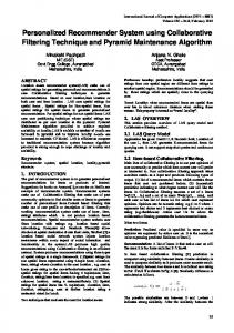
Ratings Scale Figure 1: Distribution of MovieLens dataset (ML). Furthermore, tuning parameters in RBF and polynomial kernels is very computation intensive given a large feature size. For multi class problem, several methods have been proposed, such as one-verse-one (1v1), one-verseall (1vR), Directed Acyclic Graph (DAG) [36]. We did not find any significant difference between the results obtained by 1v1 and 1vR and DAG, hence we show results in case of 1v1 only.

4

Combining Item-Based CF and Classification approaches for Improved Recommendations

We gave a simple generalized algorithm for combining the classification approach with CF. We first show how a Naive Bayes classification approach can be combined with CF, and then show how SVM (or other classification approaches) can be combined with CF.

4.1

Combining Item-Based CF and Naive Bayes Classifier (RecN BCF )

We propose a framework for combining the item-based CF with the Naive Bayes classifier. The idea is to train Naive Bayes classifier in off-line stage for generating recommendations. The prediction computed by the itembased CF using on-line stage is used if we have less confidence in the prediction computed by the Naive Bayes, else Naive Bayes’s prediction is used. We propose a simple approach for determining the confidence in the Naive Bayes’s prediction. Let PˆN B , PÎCF , and PˆF inal represent the predictions generated by the Naive Bayes classifier, item-based CF, and the prediction we are confident to be accurate. Let P r(Cj ) be the posterior probability of class j computed by the Naive Bayes classifier, L be a list containing the probabilities of each class, and d(i, j) be the absolute difference between two class probabilities, i.e. d(i, j) =

8.53 3

4

5

Rating Scale Figure 2: Distribution of FilmTrust dataset. Rating scale shown by 1, represents the counts of ratings 1 and 2; 2, represents the counts of ratings 3 and 4; 3, represents the counts of ratings 5 and 6; 4, represents the counts of ratings 7 and 8; and 5, represents the counts of ratings 9 and 10. |L(i) − L(j)| = |P r(Ci ) − P r(Cj )| where i 6= j. The proposed hybrid approach is outlined in algorithm 1. Step 2 to 5 (PÎCF = 0) represent the case, where itembased CF fails to make a prediction17 . In this case, we use prediction made by the Naive Bayes classifier. Step 7 to 16 determine the confidence in Naive Bayes’s prediction. Confidence in Naive Bayes’s prediction is high when the posterior probability of the predicted class is sufficiently larger than others. If d(S, S − 1) is sufficiently large, then we can assume that the actual value of an unknown rating has been predicted. The parameter α represents this difference and can be found empirically on training set. The parameter β tells us if the difference between the predictions made by the individual recommender systems is small, then again we are confident that Naive Bayes is able to predict a rating correctly. This is a kind of heuristic approach learnt from the prediction behaviour of CF and Naive Bayes. CF gives prediction in floating point scale, and Naive Bayes gives in integer point scale. CF recommender systems give accurate recommendation, but mostly they do not predict actual value, for example, if the actual value of an unknown rating is 4, then CF’s prediction might be 3.9 (or 4.1, or some other value). On the other hand, Naive Bayes can give actual value, for example in the aforementioned case, it might give us 4. However, if Naive Bayes is not very confident, then it might result in prediction that is not close to the actual one, e.g. 3, 2, etc. We take the difference of individual recommender’s predictions, and if it is less than a threshold (β), then we use Naive Bayes’s prediction assuming 17 This can occur when no similar item is found against a target item, for example, in new-item cold start scenario—when only the active user has rated the target item.



that it has been predicted correctly. Steps 17 to 28 represent the case, where we have tie cases in Naive Bayes posterior probabilities. In this scenario, we take difference of each tie class with CF’s prediction and use that class as final prediction, if the difference is less than β. Step 29 to 30 describe the case where we do not have enough trust in Naive Bayes’s prediction, hence we use prediction made by the item-based CF. Algorithm 1 RecN BCF 1: 2: 3: 4: 5: 6:

7: 8: 9: 10: 11: 12: 13: 14: 15: 16: 17: 18: 19: 20: 21: 22: 23: 24: 25: 26: 27: 28: 29: 30: 31:

4.2

procedure Recommend(PÎCF , PˆN B , L) if (PÎCF == 0) then a. PˆF inal ← PˆN B b. return PˆF inal end if Sort the list L in ascending order, so that L(1) contains the lowest value and L(S) contains the highest value. if (L(S) 6= L(S − 1)) then if d(S, S − 1) > α then a. PˆF inal ← PˆN B b. return PˆF inal else if (|PˆN B − PÎCF | < β) then a. PˆF inal ← PˆN B b. return PˆF inal end if end if else (i.e. L(S) = L(S − 1)) for t ← S − 1, 1 do if (L(S) == L(t)) then if (|PÎCF − t| < β) then a. PˆF inal ← t b. return PˆF inal end if else Break for end if end for end if PˆF inal ← PÎCF return PˆF inal end procedure

Combining Item-Based CF and SVM Classifier (RecSV M CF )

Algorithm 1 can be used to combine the Item-based CF and SVM classifiers. The methodology is the same, except P r(Cj ) represents the SVM’s estimated probability for the class j. Parameters can be learned in the training set through cross validation. Similarly any other classifier can be combined with collaborative filtering.

5 5.1

Experimental Evaluation Dataset

We used MovieLens (ML) and FilmTrust (FT) datasets for evaluating our algorithm. MovieLens data set contains 943 users, 1682 movies, and 100 000 ratings on an integer scale 1 (bad) to 5 (excellent). MovieLens data set has been used in many research projects [11, 41, 27]. The sparsity of this dataset is 93.7% 100000 = 0.937 . 1 − non zero entries =1 − 943×1682 all possible entries

We created the second dataset by crawling the FilmTrust website. The dataset retrieved (on 10th of March 2009) contains 1214 users, 1922 movies, and 28 645 ratings on a floating point scale of 1.0 (bad) to 10.0 (excellent). The sparsity of this dataset is 99.06%. We digitized the rating scale between 1 to 10 by rounding off a rating to the nearest integer value. The distribution of the data is shown in figure 1 and figure 218 .

5.2

Feature Extraction and Selection

We downloaded information about movies given in MovieLens and FilmTrust dataset from IMDB. After stop word removal and stemming, we constructed a vector of keywords, tags, directors, actors/actresses, and user reviews given to a movie in IMDB. We used TF-IDF approach for determining the weights of words in a document (i.e. movie) with DF-Thresholding feature selection. DF Thresholding approach computes the Document Frequency (DF ) for each word in the training set and removes words having DF less than a predetermined threshold [36]. The assumption behind this is that, these rare words neither have the discriminating power for a category prediction nor do they influence the global performance. We normalize the data between 0 and 1. It must be noted that the text categorization and recommender system share a number of characteristics. A vector space model is the most commonly used document representation technique, in which documents are represented by vectors of words. Each vector component represents a word feature and approaches, such as boolean weights, T F − IDF , normalized T F − IDF [34] etc. can be used for determining the weight of a word in document. The resulting representation also called attribute-value representation, can be very large (e.g. 10 000 dimensions and more), because there is one dimension for each unique word found in the collection of documents after stop word removal and stemming. A word-by-document matrix is used to represent a collection of documents, where each entry symbolizes the occurrence of a word in a document. This matrix is typically very sparse, as not every word appears in every document. The recommender systems share the same characteristic. In [24] the 18 Both dataset can be downloaded https://sourceforge.net/projects/hybridrecommend.


from:


authors argues that each user can be viewed as a document and each item rated by a user can be represented by a word appearing in a document. Our assumption is slightly different from the one in [24] we view each user as a document, however we get features (words) against each item rated by a user. Each item is represented by a vector of bags of words and user profile is represented by a big vector obtained by concatenating the vectors of bags of words of each item rated by the user. In this way, a user profile captured by a recommender system is very similar to the vector space model in text categorization. Hence, our assumption is that the basic text categorization algorithms can be applied to recommender system problem and that the results should be comparable.

5.3

Metrics

Several metrics have been used for evaluating recommender systems which can broadly be categorized into predictive accuracy metrics, classification accuracy metrics, and rank accuracy metrics [42]. The predictive accuracy metrics measure how close is the recommender system’s predicted value of a rating, with the true value of that rating assigned by the user. These metrics include mean absolute error, mean square error, and normalized mean absolute error, and have been used in research projects such as [13, 43, 12, 11]. The classification accuracy metrics determine the frequency of decisions made by a recommender system, for finding and recommending a good item to a user. These metrics include precision, recall, F 1 measure, and receiver operating characteristic curve, and have been used in [12, 44]. The last category of metrics, rank accuracy metrics measure the proximity between the ordering predicted by a recommender system to the ordering given by the actual user, for the same set of items. These metrics include half-life utility metric proposed by Brease [13]. Our specific task in this paper is to predict scores for items that already have been rated by actual users, and to check how well this prediction helps users in selecting high quality items. Keeping this into account, we use Mean Absolute Error (MAE) and Receiver Operating Characteristic (ROC) sensitivity. MAE measures the average absolute deviation between a recommender system’s predicted rating and a true rating assigned by the user. The goal of a recommendation algorithm is to minimize MAE. It is computed as follows:

|E| =

O X

|pi − ai |

i=1

O

,

where pi and ai are the predicted and actual values of a rating respectively, and O is the total number of samples in the test set. A sample is a tuple consisting of a user

ID, movie ID, and rating, < uid, mid, r >, where r is the rating a recommender system has to predict. It has been used in [13, 11, 29, 3, 45]. ROC is the extent to which an information filtering system can distinguish between good and bad items. ROC sensitivity measures the probability with which a system accept a good item. The ROC sensitivity ranges from 1 (perfect) to 0 (imperfect) with 0.5 for random. To use this metric for recommender systems, we must first determine which items are good (signal ) and which are bad (noise). In [46, 37] the authors consider a movie “good” if the user rated it with a rating of 4 or higher and “bad” otherwise. The flaw with this approach is that it does not take into account the inherent difference in the user rating scale—a user may consider a rating of 3 in a 5 point scale to be good, while another may consider it bad. We consider an item good if a user rated it with a score higher than their average (in the training set) and bad otherwise. It has been used in [29, 3]. Furthermore, we used coverage that measures how many items a recommender system can make recommendation for. It has been used in [42, 29, 3, 45]. We did not take coverage as the percentage of items that can be recommended/predicted from all available ones. The reason is, a recommendation algorithm can increase coverage by making bogus predictions, hence coverage and accuracy must be measured simultaneously. We selected only those items that have already been rated by the actual users.

5.4

Evaluation Methodology

We performed 5-fold cross validation and reported the average results. Each distinct fold contains 20% randomly ratings of each user as the test set and the remaining 80% as the training set. We further subdivided our training set into a validation set and training set for measuring the parameters sensitivity. For learning the parameters, we conducted 5-fold cross validation on the 80% training set, by selecting the different test and training set each time, and taking the average of results.

6

Result and Discussion

We compared our algorithm with eight different algorithms: user-based CF using Pearson correlation with default voting (U BCFDV ) [13], item-based CF (IBCF) using adjusted-cosine similarity19 [11], a hybrid recommendation algorithm, IDemo4, proposed in [27], a Naive Bayes classification approach (NB) using item content information, a SVM classification approach using item content information, two Naive hybrid approaches (NBIBCF, SVMIBCF) for generating recommendation by taking the average of the prediction generated by a 19 With the exception that we used adjusted cosine similarity, and significant weights. For more information, refer to [45].



0.84

Mean Absolute Erorr (MAE)

0.83

0.82

0.81

0.8

0.79

0.78

0.77

1.00E-05

1.00E-03

1.00E-04

1.00E-02

1.00E-01

1.00E+00

1.00E+01

1.00E+02

1.00E+03

1.00E+04

1.00E+05

Parameter C (Log Scale)

Figure 3: Determining the optimal value of parameter C in SVM for MovieLens (ML) dataset. X-axis shows the value of C in log scale. The corresponding MAE is shown on y-axis. The MAE decreases with the increase in the value of C, and becomes stable after C = 2−9 .

Mean Absolute Error (MAE)

Naive Bayes and an item-based CF, and SVM and itembased CF, and content-boosted algorithm (CB) proposed in [18]. Furthermore, we tuned all algorithms for the best mentioning parameters.

6.1

Learning the Optimal Values of Parameters

The purpose of these experiments is to determine, which of the parameters affect the prediction quality of the proposed algorithms, and to determine their optimal values.

0.77 0.765

6.1.1

0.76 0.755 0.75

Finding the Optimal Number of Neighbours (K) in Item-based Collaborative Filtering

0.745 0.74 0.735

5

10

15

20

25

30

35

40

45

50

40

45

50


Neighbourhood Size (ML Dataset) 1.5 1.49 1.48 1.47 1.46 1.45 1.44 5

10

15

20

25

30

35

Neighbourhood Size (FT Dataset)

Figure 4: Determining the optimal value of neighbourhood size (K) for MovieLens (ML) and FilmTrust (FT) dataset.

To measure the optimal number of neighbours, we changed the neighbourhood size from 5 to 50 with a difference of 5, and observed the corresponding MAE. Figure 4 shows that MAE decreases in general with the increase in the neighbourhood size. This is in contrast with the conventional item-based CF proposed in [11], where the MAE increases with the increase in the neighbourhood size. The reason is that the authors in [11] did not use any significant weighting scheme and used weighted sum prediction generation formula, whereas, we are using significant weighting schemes and adjusted weighted sum prediction generation formula20 . Figure 4 shows that the MAE keeps on decreasing with the increase in the number of neighbours, reaches at its minimum for K = 30 for MovieLens dataset and K = 25 for FilmTrust dataset, and then either starts increasing (though incre20 The

detail is not in the scope of this work, please refer to [45].




Table 1: A comparison of the proposed algorithms with others in terms of cost (based on [41]), accuracy metrics, and coverage. IBCFSW represents IBCF with significant weights applied over the rating similarity. The best results have been shown in bold. Best MAE ROC-Sensitivity Coverage Algorithm On-line Cost (ML) (FT) (ML) (FT) (ML) (FT) U BCFDV O(M 2 N ) + O(N M ) 0.743 1.448 0.714 0.502 99.789 93.611 IBCF O(N 2 ) 0.755 1.449 0.674 0.521 99.867 95.100 IBCFSW O(N 2 ) 0.744 1.425 0.787 0.530 99.867 95.100 IDemo4 O(N 2 ) 0.745 1.422 0.739 0.528 99.991 95.407 RecN BCF O(N 2 ) + O(N f ) 0.696 1.368 0.785 0.542 100 99.992 RecSV M CF O(N 2 ) + O(N nsv ) 0.684 1.346 0.793 0.536 100 99.992 NB O(N f ) 0.815 1.471 0.708 0.515 100 99.992 SVM O(N nsv ) 0.779 1.463 0.699 0.512 100 99.992 NBIBCF O(N 2 ) + O(N f ) 0.768 1.458 0.717 0.526 100 99.992 SVMIBCF O(N 2 ) + O(N nsv ) 0.759 1.445 0.723 0.534 100 99.992 CB O(M 2 N ) + O(N M ) + O(N f ) 0.711 1.393 0.748 0.531 100 99.995

1.05 1 0.95 0.9 0.85 0.8

0

0.1

0.2

0.3

0.4

0.5

0.6

0.7

0.8

0.9

1


DF Threshold (ML Dataset) 1.54

varied the value of C from 2−15 to 215 by increasing the power by 2. Figure 3 shows that the MAE is large for the small value of C, which may be due to under fitting. The MAE decreases with the increase in the value of C, reaches at its minimum for C = 2−9 , and then becomes stable for C > 2−9 (between 1.00E −03 and 1.00E −02 in log scale). We choose C = 2 for MovieLens dataset to avoid any over fitting and under fitting of the model. FilmTrust dataset shows the similar results (not shown), hence we choose C = 2 as an optimal value for FilmTrust dataset.

1.52

1.5

6.1.3

1.48

1.46

Finding the Optimal Value of DF Threshold for Naive Bayes Classifier

ment is very small) again or stays constant. For the subsequent experiments, we choose K = 30 for MovieLens and K = 25 for FilmTrust dataset as optimal neighbourhood size.

For determining the optimal value of DF , we varied the value of DF from 0 to 1.0 with a difference of 0.0521 . The results are shown in figure 5. Figure 5 shows that DF = 0.50 and DF = 0.30 gave the lowest MAE for MovieLens and FilmTrust dataset respectively. It is worth noting that, the values of parameters are found to be different for MovieLens and FilmTrust dataset, which is due to the fact that both dataset have different density, rating distribution, and rating scale. We choose these values of DF for the subsequent experiments.

6.1.2

6.1.4

0

0.1

0.2

0.3

0.4

0.5

0.6

0.7

0.8

0.9

1

DF Threshold (FT Dataset)

Figure 5: Determining the optimal value of DF for MovieLens (ML) and FilmTrust (FT) dataset.

Finding the Optimal Value of C for SVM

The cost parameter, C, controls the trade off between permitting training errors and forcing rigid margins. It allows some misclassification by creating soft margins. A more accurate model can be created by increasing the value of C that increases the cost of misclassification, however the resulting model may over fit. Similarly, a small value of C may under fit the model. Figure 3 shows, how MAE changes with the change in the value of C. We

Finding the Optimal Value of DF Threshold for SVM

For determining the optimal value of DF , we varied the value of DF from 0 to 1.0 with a difference of 0.05. The results (not shown) did not show any improvement. We did not perform any feature selection for SVM. 21 DF = 0.05 means that the word should occur at-least in 5% of the movies seen by an active user, to be considered as a valid feature.



0.86 0.84

0.76

0.8



0.78 0.82

0.78 0.76 0.74 0.72 0.7 0.68

0.74

0.72

0.7

0.68

0 0.1

0.66

0.2

0

0.3

0.1 0.4

0.4

0.2 0.5 0.35

0.6

0.7

0.1 1

Parameter Beta

0.2

0.6

0.15 0.9

0.25

0.5

0.25 0.2

0.8

0.3

0.4

0.3 0.7

0.35

0.3

0.4

0.15 0.8

0.05

0.1 0.9

0

0.05 1

Parameter Alpha

0

Parameter Alpha Parameter Beta

Figure 6: Finding the optimal value of α and β in RecN BCF , through grid search. 6.1.5

Finding the Optimal Value of α and β for RecN BCF Algorithm

For MovieLens dataset, we performed a series of experiments by changing α from 0.02 to 0.4 with a difference of 0.02. For each experiment, we changed β from 0.05 to 1.0 with difference of 0.05, keeping the α parameter fixed, and observed the corresponding MAE. The grid coordinates which gave the lowest MAE are recorded to be the optimal parameters. Figure 6 shows that the MAE decreases with the increase in the value of alpha and reaches it peak at α = 0.34. After that it either increases or stays constant. We note that the MAE is minimum between β = 0.7 to β = 0.8. Keeping the results in account, we choose the optimal value of α and β to be 0.34 and 0.7 respectively. For FilmTrust dataset, the optimal parameters are found to be α = 0.20 and β = 0.9. We note that the values of parameters are found different for MovieLens and FilmTrust dataset.

6.1.6

Finding the Optimal Value of α and β for RecSV M CF Algorithm

For MovieLens dataset, we performed a series of experiments by changing α from 0.02 to 0.4 with a difference of 0.02. For each experiment, we changed β from 0.05 to 1.0 with difference of 0.05, keeping the α parameter fixed, and observed the corresponding MAE. Again, the grid coordinates which gave the lowest MAE are recorded to be the optimal parameters. Figure 7 shows that the

Figure 7: Finding the optimal value of α and β in RecSV M CF , through grid search. MAE decreases with the increase in the value of alpha and reaches it peak at α = 0.36. After that it either increases or stays constant. We note that at β = 0.7, the MAE is minimum. Keeping the results in account, we choose the optimal value of α and β to be 0.36 and 0.7 respectively. For FilmTrust dataset, the optimal parameters are found to be α = 0.25 and β = 0.85. We note that the values of parameters are found different for MovieLens and FilmTrust dataset.

6.2 6.2.1

Performance Evaluation With Other Algorithms Performance Evaluation in Terms of MAE, ROC-Sensitivity, and Coverage

The MAE, ROC-sensitivity, and coverage of the proposed algorithms are shown in table 1. Table 1 shows that the proposed algorithms outperform other significantly in terms of MAE and ROC-sensitivity, whereas they give comparable results to others in terms of coverage metric. The reason for such good results is that when a classifier has sufficiently large confidence in prediction, then it can correctly classify an instance (a unknown rating), resulting in the reduced MAE, and increased ROC-sensitivity and coverage. The percentage improvement, in case of RecN BCF , over NBIBCF is 9.2% and 6.17% for MovieLens and FilmTrust dataset respectively. The percentage improvement, in case of RecSV M CF , over SVMIBCF is 9.8% and 6.8% for MovieLens and FilmTrust dataset respectively. These results indicate that our algorithms give



statistically significant results than the naive approaches used to combine the classifiers and CF. It is worth noting that for FilmTrust dataset, ROC sensitivity is lower, for all algorithms in general, as compared to MovieLens dataset. We believe that it is due to the rating distribution. Furthermore, the coverage of the algorithms is much lower in the case of FilmTrust dataset, which is due to the reason that it is very sparse.

6.2.2

Performance Evaluation Under Cold-Start Scenarios

We checked the performance of the algorithm under new item cold-start problems. When an item is rated by only few users, then item-based and user-based CF will not give good results. Our proposed scheme works well in new item cold-start problem scenario, as it does not solely depend on the number of users who have rated the target item for finding the similarity. We assume that itembased CF fails to make prediction, if the target item is rated by very few users (γ). The parameter γ is learned through the training set, and is found to be 10 for MovieLens and 8 for FilmTrust dataset. This value of γ indicates that under new-item cold-start scenario, it is better to use classification approach rather than CF approach. For testing our algorithm in this scenario, we selected 1000 random samples of user/item pairs from the test set. While making prediction for a target item, the number of users in the training set who have rated target item were kept 0, 2, and 5. The corresponding MAE ; represented by MAE 0, MAE 2, MAE 5, is shown in table 2. Table 2 shows that CF and IDemo4 fail to make prediction when only the active user rated the target item, and in general they gave inaccurate predictions. It is worth noting that, in e-commerce domains (e.g. Amazon), there may be millions of items that are rated by only a few users (< 5). In this scenario, CF and related approaches would results in inaccurate recommendations. The poor performance of user-based CF is due to the reason that, we have less neighbours against an active user, hence performance degrades. The reason in case of item-based CF is that, the similar items found after applying rating correlation may be not actually similar. As while finding similarity, we isolate all users who have rated both target item and the item we find similarity with. In this case, we have maximum 5 users who have rated both items, as a result, similarity found by adjusted cosine measure will be misleading. The IDemo4 produces poor results, as it operates over candidate neighbouring items found after applying the rating similarity. Both content-boosted and the proposed approaches give good results as they make effective use of user’s content profile that can be used by a classifier for making predictions. It must be noted that our algorithm will not give good

results in the case of new user cold-start problems. The reason is that we do not have enough training data to train classifiers. This problem can effectively be solved by applying the vector similarity [13] over user or item’s content profiles to find similar users or items, which can be used for making predictions. Alternatively, user content profiles can be matched with item content profiles to generate recommendations.

6.2.3

Performance Evaluation In Terms of Cost

Table 1 shows the on-line cost22 of different algorithms used in this work. Here, f is the number of features/words in the dictionary (used in a classifier). The training computation complexity of SVM and Naive Bayes classifier, for one user, is O(N 3 ) and O(N f ) respectively. We train M classifiers, so total training computation complexity becomes O(M N 3 ) for SVM and O(M N f ) for Naive Bayes. The classifying computation complexity for one sample (rating) is O(nsv ) for SVM and O(f ) for Naive Bayes. If we classify N items then it becomes O(N nsv ) for SVM and O(N f ) for Naive Bayes. Table 1 shows that the proposed algorithms are scalable and practical as their on-line cost is less or equal to the cost of other algorithms. We are using item-based CF, whose on-line cost is less than that of user-based CF used in [18]23 . Even if we consider using Naive Bayes classifier to fill the user-item rating matrix and then use item-based CF over this filled matrix, then our cost will be less than that. The reason is, in the filled matrix case, one has to go through all the filled rows of matrix for finding the similar items. For a large e-commerce system like Amazon, where we already have millions of neighbours against an active user/item, filling the matrix and then going through all the users/items for finding the similar users/items in not pragmatic due to limited memory and other constraint on the execution time of the recommender system.

6.3

Eliminating Over Specialization Problem: Producing Diverse Recommendations

Pure content-based recommender systems recommend items that are the most similar to a user’s profile. In this way, a user can not find recommendations that are different from the ones it has already rated or seen. The proposed algorithms can overcome the over-specialization problem caused by pure content-based filtering. The reason is that they do not totally depend on classifi22 It is the cost for generating predictions for N items. We assume that we compute item similarities and train classifier in off-line fashion. 23 It is because, we can build expensive and less volatile item similarity model in off-line fashion. Hence on-line cost becomes O(N 2 ) in worst case, and in practical it is O(KN ), where K is the number of top K most similar items against a target item (K < N ).



Table 2: Performance evaluation under new item cold-start problem. If the number of users who have rated the target item is zero, then the conventional approaches fail to produce recommendation. The table shows that the proposed approaches produce more accurate recommendations than the conventional ones. The best results have been shown in bold. MAE0 MAE2 MAE5 Algo. (ML) (FT) (ML) (FT) (ML) (FT) U BCFDV – – 1.229 2.197 0.920 1.801 IBCFSW – – 1.192 2.152 0.864 1.742 IDemo4 – – 1.171 2.123 0.849 1.714 CB 0.830 1.491 0.815 1.476 0.802 1.465 RecN BCF 0.809 1.478 0.809 1.478 0.809 1.478 RecSV M CF 0.791 1.467 0.791 1.467 0.791 1.467

cation algorithms trained on the content information. They can make recommendation outside the preferences (outside the box [19]) of an individual by switching to the CF recommendation approach. Diversity [42] of recommendations is very important, and a system should not recommend items to users that are very similar to the previously recommended items. If we construct a list of top-N recommendation for an active user, then our algorithms would introduce some sort of randomness in the recommendation list, resulting in a range of alternatives to be recommended rather than homogeneous set of alternatives. By switching to machine learning classifiers and CF approaches, our algorithms can balance the accuracy and diversity of recommendations.

7

Conclusion And Future Work

In this paper, we have proposed a switching hybrid recommendation approach by combining item-based collaborative filtering with a classification approach. We empirically show that our recommendation approach outperform others in terms of accuracy, and coverage and is more scalable. As a future work, we would like to use over sampling and under sampling [36] schemes to overcome the imbalanced dataset problem. We note in figures 1 and 2 that the distribution of the data is skewed towards the higher ratings, hence results of a classifier may be biased. In our work, we overcome imbalanced dataset problem for SVM classification, by assigning different penalties to classes according to the prior knowledge of users. The prior knowledge of a user is the fraction of the total number of ratings belonging to a class to the total number of ratings provided by the user in the training set. Another important area of research is to use regression rather than classification approaches, which may increase the performance of our hybrid system. Moreover, different feature selection algorithms can be used to enhance the performance of classifiers. Another interesting area of future research is to apply di-

mensionality reduction techniques to reduce the dimensions of the dataset. Partitional clustering algorithms, such as KMeans clustering [47], or singular value decomposition [12] can be applied over the user-item rating matrix to reduce the dimensionality of the dataset. CF can be applied over the clustered data, making the resulting system scalable. Finally, individual predictions made by user-based and item-based CF can be combined in switching hybrid way. We hope that combining these two approaches will result in increase in accuracy, as both of them focus on different kind of relationship. In certain cases, user-based CF may be useful in identifying different kind of relationship that item-based CF will fail to recognize, for example, if none of the items rated by an active user are closely related to the target item nt , then it is beneficiary to switch to user-oriented perspective that may find set of users very similar to the active user, who rated target item nt . Combining these approaches with classification ones can further increase the performance of our algorithms. Furthermore, we would like to evaluate our algorithms on dataset of domains other than movies, such as BookCrossing24 dataset.

Acknowledgment The work reported in this paper has formed part of the Instant Knowledge Research Programme of Mobile VCE, (the Virtual Centre of Excellence in Mobile & Personal Communications), www.mobilevce.com. The programme is co-funded by the UK Technology Strategy Boards Collaborative Research and Development programme. Detailed technical reports on this research are available to all Industrial Members of Mobile VCE. This work has been supported from UET-Taxila (www.uettaxila.edu.pk) Pakistan. We would like to thank Juergen Ulbts (http://www.jmdb.de/) and Martin Helmhout for helping integrating datasets with IMDB. 24 http://www.informatik.uni-freiburg.de/


cziegler/BX/


References [1] P. Resnick and H. R. Varian, “Recommender systems,” Commun. ACM, vol. 40, no. 3, pp. 56–58, 1997.

[12] B. Sarwar, G. Karypis, J. Konstan, and J. Riedl, “Application of dimensionality reduction in recommender system–a case study,” in ACM WebKDD 2000 Web Mining for E-Commerce Workshop. Citeseer, 2000.

[2] B. Mobasher, “Recommender systems,” Kunstliche Intelligenz, Special Issue on Web Mining, vol. 3, pp. 41–43, 2007.

[13] J. S. Breese, D. Heckerman, and C. Kadie, “Empirical analysis of predictive algorithms for collaborative filtering.” Morgan Kaufmann, 1998, pp. 43–52.

[3] M. Ghazanfar and A. Prugel-Bennett, “An Improved Switching Hybrid Recommender System Using Naive Bayes Classifier and Collaborative Filtering,” in Lecture Notes in Engineering and Computer Science: Proceedings of The International Multi Conference of Engineers and Computer Scientists 2010. IMECS 2010, 17–19 March, 2010, Hong Kong, pp. 493–502. [4] J. Y. G Linden, B Smith, “Amazon.com recommendations: item-to-item collaborative filtering,” in IEEE, Internet Computing, vol. 7, 2003, pp. 76–80. [5] D. Goldberg, D. Nichols, B. Oki, and D. Terry, “Using collaborative filtering to weave an information tapestry,” Communications of the ACM, vol. 35, no. 12, p. 70, 1992. [6] U. Shardanand and P. Maes, “Social information filtering:algorithms for automating word of mouth,” in Proc. Conf. Human Factors in Computing Systems, 1995, pp. 210–217.

[14] Y. Park and A. Tuzhilin, “The long tail of recommender systems and how to leverage it,” in Proceedings of the 2008 ACM conference on Recommender systems. ACM New York, NY, USA, 2008, pp. 11– 18. [15] M. Pazzani and D. Billsus, “Content-based recommendation systems,” 2007, pp. 325–341. [16] K. Lang, “Newsweeder: Learning to filter netnews,” in In Proceedings of the Twelfth International Conference on Machine Learning, 1995. [17] S. Alag, Collective Intelligence in Action. Manning Publications, October, 2008. [18] P. Melville, R. J. Mooney, and R. Nagarajan, “Content-boosted collaborative filtering for improved recommendations,” in in Eighteenth National Conference on Artificial Intelligence, 2002, pp. 187– 192.

[7] L. Terveen, W. Hill, B. Amento, D. McDonald, and J. Creter, “Phoaks: A system for sharing recommendations,” in Comm. ACM, vol. 40, 1997, pp. 59–62.

[19] R. Burke, “Hybrid recommender systems: Survey and experiments,” User Modeling and User-Adapted Interaction, vol. 12, no. 4, pp. 331–370, November 2002.

[8] P. Resnick, N. Iacovou, M. Suchak, P. Bergstrom, and J. Riedl, “GroupLens: An open architecture for collaborative filtering of netnews,” in Proceedings of the 1994 ACM conference on Computer supported cooperative work. ACM New York, NY, USA, 1994, pp. 175–186.

[20] M. J. Pazzani, “A framework for collaborative, content-based and demographic filtering,” Artificial Intelligence Review, vol. 13, no. 5 - 6, pp. 393–408, December 1999.

[9] J. A. Konstan, B. N. Miller, D. Maltz, J. L. Herlocker, L. R. Gordon, and J. Riedl, “Grouplens: applying collaborative filtering to usenet news,” Commun. ACM, vol. 40, no. 3, pp. 77–87, March 1997. [10] A. T. Gediminas Adomavicius, “Toward the next generation of recommender systems: A survey of the state-of-the-art and possible extensions,” IEEE Transactions on Knowledge and Data Engineering, vol. 17, pp. 734–749, 2005. [11] B. Sarwar, G. Karypis, J. Konstan, and J. Reidl, “Item-based collaborative filtering recommendation algorithms,” in Proceedings of the 10th international conference on World Wide Web. ACM New York, NY, USA, 2001, pp. 285–295.

[21] M. Claypool, A. Gokhale, T. Mir, P. Murnikov, D. Netes, and M. Sartin, “Combining content-based and collaborative filters in an online newspaper,” in In Proceedings of ACM SIGIR Workshop on Recommender Systems, 1999. [22] R. Burke, “Integrating knowledge-based and collaborative-filtering recommender systems,” in Proceedings of the Workshop on AI and Electronic Commerce, 1999. [23] S. Al Mamunur Rashid, G. Karypis, and J. Riedl, “ClustKNN: a highly scalable hybrid model-& memory-based CF algorithm,” in Proc. of WebKDD 2006: KDD Workshop on Web Mining and Web Usage Analysis, August 20-23 2006, Philadelphia, PA. Citeseer.



[24] T. Zhang and V. Iyengar, “Recommender systems using linear classifiers,” The Journal of Machine Learning Research, vol. 2, p. 334, 2002. [25] R. J. Mooney and L. Roy, “Content-based book recommending using learning for text categorization,” in Proceedings of DL-00, 5th ACM Conference on Digital Libraries. San Antonio, US: ACM Press, New York, US, 2000, pp. 195–204. [26] M. Vozalis and K. Margaritis, “Collaborative filtering enhanced by demographic correlation,” in AIAI Symposium on Professional Practice in AI, of the 18th World Computer Congress, 2004. [27] ——, “On the enhancement of collaborative filtering by demographic data,” Web Intelligence and Agent Systems, vol. 4, no. 2, pp. 117–138, 2006. [28] Y. S. Marko Balabanovic, “Fab: content-based, collaborative recommendation,” in Communications of the ACM archive, vol. 40, Miami, Florida, USA, 1997, pp. 66–72. [29] M. A. Ghazanfar and A. Prugel-Bennett, “A scalable, accurate hybrid recommender system,” in The 3rd International Conference on Knowledge Discovery and Data Mining (WKDD 2010). IEEE, January 2010. [Online]. Available: http://eprints.ecs.soton.ac.uk/18430/ [30] B. Sarwar, J. Konstan, J. Herlocker, B. Miller, and J. Riedl, “Using filtering agents to improve prediction quality in the GroupLens research collaborative filtering system,” in Proceedings of the 1998 ACM conference on Computer supported cooperative work. ACM New York, NY, USA, 1998, pp. 345–354. [31] N. Good, J. Schafer, J. Konstan, A. Borchers, B. Sarwar, J. Herlocker, and J. Riedl, “Combining collaborative filtering with personal agents for better recommendations,” in Proceedings of the National Conference on Artificial Intelligence. JOHN WILEY & SONS LTD, 1999, pp. 439–446. [32] H. Ma, I. King, and M. Lyu, “Effective missing data prediction for collaborative filtering,” in Proceedings of the 30th annual international ACM SIGIR conference on Research and development in information retrieval. ACM, 2007, p. 46. [33] U. Nahm and R. Mooney, “Text mining with information extraction,” 2002. [34] K. Aas and L. Eikvil, “Text categorisation: A survey.” 1999. [35] I. H. Witten, G. W. Paynter, E. Frank, C. Gutwin, and C. G. Nevill-Manning, “Kea: practical automatic keyphrase extraction,” in DL ’99: Proceedings of the fourth ACM conference on Digital libraries. ACM Press, 1999, pp. 254–255.

[36] I. H. W. Witten and F. Eibe, Data Mining: Practical Machine Learning Tools and Techniques with Java Implementations. Morgan Kaufmann, October 1999. [37] K. Jung, D. Park, and J. Lee, “Hybrid Collaborative Filtering and Content-Based Filtering for Improved Recommender System,” Lecture Notes in Computer Science, pp. 295–302, 2004. [38] T. Joachims, “Text categorization with support vector machines: Learning with many relevant features.” Springer Verlag, 1998, pp. 137–142. [39] C. Hsu, C. Chang, C. Lin et al., “A practical guide to support vector classification,” 2003. [40] C.-C. Chang and C.-J. Lin, LIBSVM: a library for support vector machines, http://www.csie.ntu.edu.tw/ cjlin/libsvm, 2001. [41] M. Vozalis and K. Margaritis, “Using SVD and demographic data for the enhancement of generalized collaborative filtering,” Information Sciences, vol. 177, no. 15, pp. 3017–3037, 2007. [42] L. G. T. Jonathan L. Herlocker, Joseph A. Konstan and J. T. Riedl, “Evaluating collaborative filtering recommender systems,” ACM Transactions on Information Systems (TOIS) archive, vol. 22, pp. 734– 749, 2004. [43] B. M. Sarwar, G. Karypis, J. Konstan, and J. Riedl, “Recommender systems for large-scale e-commerce: Scalable neighborhood formation using clustering,” 2002. [44] B. Sarwar, G. Karypis, J. Konstan, and J. Riedl, “Analysis of recommendation algorithms for ecommerce.” ACM Press, 2000, pp. 158–167. [45] M. A. Ghazanfar and A. Prugel-Bennett, “Novel Significance Weighting Schemes for Collaborative Filtering: Generating Improved Recommendations in Sparse Environments,” in The 6th International Conference on Data Mining 2010 (DMIN 10), 2010. [Online]. Available: http://eprints.ecs.soton.ac.uk/18788/ [46] J. Herlocker, J. Konstan, and J. Riedl, “An algorithmic framework for performing collaborative filtering,” in Proceedings of the 22nd annual international ACM SIGIR conference on Research and development in information retrieval. ACM New York, NY, USA, 1999, pp. 230–237. [47] P. Berkhin, “Survey of clustering data mining techniques,” 2002.
