1 FEBRUARY 2004
FEDOROVICH ET AL.
281
Convective Entrainment into a Shear-Free, Linearly Stratified Atmosphere: Bulk Models Reevaluated through Large Eddy Simulations EVGENI FEDOROVICH
AND
ROBERT CONZEMIUS
School of Meteorology, University of Oklahoma, Norman, Oklahoma
DMITRII MIRONOV German Weather Service, Offenbach am Main, Germany (Manuscript received 19 December 2002, in final form 15 September 2003) ABSTRACT Relationships between parameters of convective entrainment into a shear-free, linearly stratified atmosphere predicted by the zero-order jump and general-structure bulk models of entrainment are reexamined using data from large eddy simulations (LESs). Relevant data from other numerical simulations, water tank experiments, and atmospheric measurements are also incorporated in the analysis. Simulations have been performed for 10 values of the buoyancy gradient in the free atmosphere covering a typical atmospheric stability range. The entrainment parameters derived from LES and relationships between them are found to be sensitive to the model framework employed for their interpretation. Methods of determining bulk model entrainment parameters from the LES output are proposed and discussed. Within the range of investigated free-atmosphere stratifications, the LES predictions of the inversion height and buoyancy increment across the inversion are found to be close to the analytical solutions for the equilibrium entrainment regime, which is realized when the rate of time change of the CBL-mean turbulence kinetic energy and the energy drain from the CBL top are both negligibly small. The zero-order model entrainment ratio of about 0.2 for this regime is generally supported by the LES data. However, the zero-order parameterization of the entrainment layer thickness is found insufficient. A set of relationships between the general-structure entrainment parameters for typical atmospheric stability conditions is retrieved from the LES. Dimensionless constants in these relationships are estimated from the LES and laboratory data. Power-law approximations for relationships between the entrainment parameters in the zero-order jump and general-structure bulk models are evaluated based on the conducted LES. In the regime of equilibrium entrainment, the stratification parameter of the entrainment layer, which is the ratio of the buoyancy gradient in the free atmosphere to the overall buoyancy gradient across the entrainment layer, appears to be a constant of about 1.2.
1. Introduction The atmospheric convective boundary layer (CBL) is a particular type of turbulent boundary layer forced by buoyancy flux originating at the bottom of the layer (surface heating) or at its top (radiative cooling from clouds), or both. Buoyant convection is usually the main mechanism of turbulence production in the CBL, and the contribution of wind shear to the generation of turbulence is of secondary importance. In cases when shear production is negligible compared to the buoyancy production of turbulence within the CBL, the CBL is considered shear-free. This paper focuses on the clear (no clouds), shear-free CBL driven by buoyancy forcing only from the underlying surface. Corresponding author address: Dr. Evgeni Fedorovich, Sarkeys Energy Center, 100 East Boyd, School of Meteorology, University of Oklahoma, Norman, OK 73019-1013. E-mail:
[email protected]
q 2004 American Meteorological Society
The discussion below is presented in terms of buoyancy, defined as b 5 2g(r 2 r 0 )/r 0 , where r is the density of the fluid, r 0 is the reference density, and g is the acceleration due to gravity. The virtual potential temperature u y can be used instead of r to define buoyancy, b 5 g(u y 2 u y 0 )/u y 0 , where u y 0 is the reference value of u y since, in most atmospheric cases, the two can be assumed to be linearly related. The CBL can be subdivided into three separate layers: the surface layer, in which the buoyancy decreases fairly rapidly with height; the mixed layer, where mean vertical buoyancy gradients are near zero; and the entrainment zone (also referred to as the inversion layer or interfacial layer), where buoyancy once again increases significantly with height. Further details about CBL structure are provided in several atmospheric boundary layer textbooks. This paper focuses on the entrainment zone in which air from the free atmosphere, which is more buoyant than the CBL air, is entrained across the inversion layer into the convectively mixed layer as the
282
JOURNAL OF THE ATMOSPHERIC SCIENCES
CBL grows. Such convective entrainment is maintained by the penetration of thermals into the stably stratified atmosphere above the CBL and subsequent folding of more buoyant air from aloft into the CBL, as these overshooting thermals sink back into the mixed layer. The rate of convective entrainment in the clear CBL depends most critically on the buoyancy stratification in the free atmosphere above the CBL (Sorbjan 1996) and the magnitude of buoyancy flux at the lower surface. In atmospheric models of convective entrainment, the vertical buoyancy distribution in the free atmosphere is commonly taken to be linear (at least locally) and continuous (Zilitinkevich et al. 1992; Stevens and Lenschow 2001). The CBL development and convective entrainment in a continuously and linearly stratified atmosphere have been extensively studied during special field campaigns (e.g., Chorley et al. 1975; Kaimal et al. 1976; Caughey and Palmer 1979; Caughey 1982; Boers et al. 1984; Stull and Eloranta 1984; Boers and Eloranta 1986; Boers 1989; Nelson et al. 1989; Batchvarova and Gryning 1991, 1994; Gryning and Batchvarova 1994; Lenschow 1998), in laboratory models of the atmospheric CBL and related flow types (e.g., Turner 1968; 1973; Deardorff et al. 1969; Willis and Deardorff 1974; Deardorff et al. 1980; Deardorff and Willis 1985; Fernando 1991; Fedorovich et al. 1996; McGrath et al. 1997; Fedorovich and Kaiser 1998; Fedorovich et al. 2001a,b), with bulk CBL models (e.g., Ball 1960; Lilly 1968; Plate 1971; Betts 1973; Carson 1973; Tennekes 1973; Stull 1973; Betts 1974; Carson and Smith 1974; Zilitinkevich 1975, 1991; Zeman and Tennekes 1977; Deardorff 1979; Driedonks 1982; Driedonks and Tennekes 1984; Fedorovich 1995; Fedorovich and Mironov 1995; Fedorovich 1998), and by numerical simulations (e.g., Deardorff 1970a, 1974; Sorbjan 1996; Lewellen and Lewellen 1998; Sullivan et al. 1998; Lock and MacVean 1999; van Zanten et al. 1999; Fedorovich et al. 2001a,b; Stevens and Lenschow 2001; Fedorovich and Tha¨ter 2001; Otte and Wyngaard 2001). Nevertheless, a consensus has not been reached regarding the dependence of the integral parameters of convective entrainment on the capping inversion strength and static stability in the free atmosphere. These integral parameters are the CBL growth rate (also called the entrainment rate), the entrainment ratio (the ratio of the buoyancy flux of entrainment to the surface buoyancy flux), and the relative entrainment layer depth (the ratio of the entrainment layer depth to that of the CBL). Convective entrainment in the linearly stratified atmosphere has been extensively examined within the framework of the zero-order jump bulk model (ZOM). The ZOM was introduced in Lilly (1968), used extensively in Zilitinkevich (1991) to investigate particular regimes of shear-free penetrative convection, and generalized in Fedorovich (1995). The ZOM parameterizes the inversion layer by an interface of infinitesimally small thickness in which buoyancy and buoyancy flux, averaged over horizontal planes and/or in time, have
VOLUME 61
zero-order discontinuities. More recently, Lilly (2002) suggested that local profiles of buoyancy and buoyancy flux may actually resemble the ZOM parameterization very closely and that the differences between ZOM and horizontally averaged profiles of buoyancy and buoyancy flux may disappear if a transformed coordinate system is used. Details of the ZOM methodology and associated entrainment parameterizations are provided in the next section. Inspired by Deardorff’s (1979) ideas, Fedorovich and Mironov (1995) developed a general-structure model (GSM) of entrainment. The model is based on a selfsimilar representation of the buoyancy profile within the entrainment zone that in GSM, unlike in ZOM, has a finite nonzero thickness. Details of the GSM are also given in the next section. The GSM model provided an explanation for some ambiguous relationships between the entrainment parameters in the water tank experiments of Deardorff et al. (1980), but it has not yet been tested against large eddy simulation (LES) data. In the present study, the relationships between the integral parameters of convective entrainment in the linearly stratified atmosphere are investigated numerically, by means of a large eddy simulation. Data from other numerical and experimental studies are also used in the analysis. The investigated ranges of the CBL depth and the stratification strength cover most of their atmospheric variability. Output of the LES is interpreted in terms of the bulk models and compared with analytical solutions of the ZOM for the particular regime of equilibrium (quasi stationary) entrainment. The regime of equilibrium entrainment is realized when the rate of time change of the CBL-mean turbulence kinetic energy and the energy drain from the CBL top are both negligibly small. The occurrence of this regime, which is characterized by a constant value of the entrainment ratio, is verified through numerical solutions. Entrainment predictions by the ZOM and GSM are compared with entrainment characteristics derived from LES. Inherent limitations of the bulk model parameterizations of convective entrainment are demonstrated and discussed. 2. Bulk models of convective entrainment a. Zero-order jump model Under typical atmospheric conditions, three regions (sublayers) can be distinguished within the CBL: the near-surface layer, the convectively mixed layer, and the inversion layer. The mean buoyancy in the convectively mixed layer, b m , is approximately constant with respect to height. Close to the surface, the buoyancy decreases with height from its surface value to its mixed layer value, b m . The mean vertical turbulent buoyancy flux B, obtained by the horizontal and/or time averaging, decreases linearly with height in the mixed layer. Its zero-crossing height roughly corresponds to the mixed-
1 FEBRUARY 2004
283
FEDOROVICH ET AL.
with due regard for the ZOM parameterization of the vertical buoyancy profile described above, Eq. (1) yields the equation of the buoyancy budget in the CBL:
1
2
d N 2 z i2 2 z i Db 5 B s , dt 2
(2)
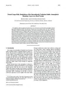
where B s is the surface value of the vertical buoyancy flux (see Fedorovich 1995 for details). To arrive at Eq. (2), the difference between the mean buoyancy in the convectively mixed layer, b m , and the actual buoyancy near the surface is neglected. Although this difference may be substantial, its contribution to the integral buoyancy budget in the CBL is small and can safely be neglected by virtue of the fact that the surface layer depth is small compared to the CBL depth. Integrating Eq. (1) over z from 0 to z 5 z i1 and taking into account Eq. (2) yield the ZOM buoyancy flux profile: FIG. 1. Representation of the buoyancy b and buoyancy flux B profiles in the ZOM and GSM, after Fedorovich and Mironov (1995). The GSM b and B profiles, which schematically are rather close to typical atmospheric b and B profiles, are shown by thin solid lines, and their ZOM counterparts are given by heavy dashed lines. See the text for notation.
layer top. Above the mixed layer, the buoyancy increases sharply with height throughout the capping inversion, and its net change over the finite depth of the interfacial layer is denoted as db. The buoyancy flux reaches a minimum at some level within the inversion and vanishes toward the upper boundary of the inversion. The ZOM representation of the vertical buoyancy profile in the atmospheric CBL (Zilitinkevich 1991; Fedorovich and Mironov 1995) is based on the aforementioned observational evidence. This representation is illustrated in Fig. 1. The mean buoyancy b is taken to be depth constant and equal to b m throughout the whole CBL. The inversion (interfacial) layer is replaced by a zero-order discontinuity surface with a buoyancy jump Db at the level z i , approximately halfway through the inversion layer (for the remainder of this paper, d refers to the net change in any time- and horizontally averaged quantity across the inversion layer, and D refers to the ZOM representation of this change). Stratification in the free atmosphere above the CBL is characterized by a positive vertical buoyancy gradient db/dz 5 N 2 , where N is the Brunt–Va¨isa¨la¨ (buoyancy) frequency. In a linearly stratified free atmosphere, at z . z i , the mean buoyancy profile is given by b 5 b m 1 Db 1 N 2 (z 2 z i ). The horizontally averaged buoyancy transport equation has the form ]b ]B 52 . ]t ]z
(1)
When integrated over the CBL depth from the surface (z 5 0) to the outer edge of the inversion layer (z 5 z i1 ),
1
B 5 Bs 1 2
2
1
2
z z z dz z 1 Bi 5 Bs 1 2 2 Db i . zi zi zi dt z i
(3)
The negative buoyancy flux at z 5 z i2 , B i [ 2Db(dz i / dt), is treated in the ZOM as the entrainment buoyancy flux (Lilly 1968). As is clear from Fig. 1, db is larger than Db for all N larger than 0, and the absolute value of the ZOM entrainment flux B i is larger than the absolute value of the actual buoyancy flux dB i in its minimum. Given the surface buoyancy flux B s and the buoyancy frequency N above the CBL, the buoyancy budget equation (2) contains two unknowns: the zero-order buoyancy increment Db (alternatively the mixed-layer buoyancy b m could be used) and the CBL depth z i . One more equation is required to close the problem, namely, the so-called entrainment equation. The method of deriving the entrainment equation differs by author. Many authors have derived it by directly relating the entrainment ratio (in some publications referred to as the entrainment coefficient) to one stratification parameter or another, or simply assuming it to be a constant. The entrainment ratio is commonly defined as the negative of the ratio of the entrainment buoyancy flux at the CBL top to the surface buoyancy flux, 2B i /B s . Note that with this method, no explicit treatment of the turbulence kinetic energy (TKE) budget is required. Indeed, the expression for the entrainment buoyancy flux, B i 5 2Db(dz i /dt), follows from the ZOM parameterization of the vertical buoyancy profile (Lilly 1968) and the budget of mean buoyancy in the CBL. An assumption on 2B i /B s immediately gives the desired equation for z i without an explicit treatment of the TKE budget in the CBL, although this budget stands behind any entrainment equation. We adhere to the approach outlined by Zilitinkevich (1991), which is based on the explicit treatment of the TKE budget and physically transparent hypotheses about the vertical profiles of the TKE and its dissipation
284
JOURNAL OF THE ATMOSPHERIC SCIENCES
VOLUME 61
rate within the CBL. In this manner, the potential and inherent limitations of the ZOM, or any other bulk model, are clarified. The entrainment equation derived by Zilitinkevich (1991) is rather general and can be applied to many regimes of entrainment in any two-layer or linearly stratified fluid. The equation can be reduced to simpler forms to describe more specific regimes of entrainment, such as the equilibrium entrainment regime considered simultaneously by Betts (1973), Tennekes (1973), and Carson (1973). We begin with the derivation of the general entrainment equation and simplify it to the case of equilibrium entrainment, which we investigate in this paper. Consider the (horizontally averaged) transport equation for the TKE in the shear-free CBL. It reads
Substituting Eqs. (6) and (7) into Eq. (5), we obtain the entrainment equation:
](Fe 1 Fp ) ]e 5B2 2 «, ]t ]z
Db(dz i /dt) 5 1 2 2C« [ C1 . Bs
(4)
where e is the TKE per unit mass, F e and F p are the vertical fluxes of energy associated with turbulent transport and pressure fluctuations, respectively (it is assumed that they both vanish at the underlying surface), and « is the TKE dissipation rate. Integration of Eq. (4) over z from z 5 0 to z 5 z i1 gives the integral TKE budget in the CBL: d dt
E
zi
e dz 5
0
1
2
zi dz B s 2 Db i 2 F i 2 2 dt
E
zi
« dz,
(5)
0
where F i 5 (F e 1 F p ) | zi1 stands for the upward energy flux at the CBL top. This flux is related to the energy drain from the CBL due to internal gravity waves propagating in the stably stratified free atmosphere aloft (Stull 1976b; Zilitinkevich 1991). Based on the Deardorff (1970b) and Zilitinkevich and Deardorff (1974) scaling considerations for the shearfree CBL, Zilitinkevich (1991) proposed a parameterization for e and « in the ZOM: e 5 w*2 we
12
z , zi
«5
12
w*3 z w , zi « zi
(6)
where w* 5 (B s Z i )1/3 is the Deardorff (1970a,b) convective velocity scale and w e , w« are dimensionless universal functions of the dimensionless height, z 5 z/z i . These functions integrate to two universal constants:
E
1
Ce 5
0
E
1
we (z ) dz and C « 5
w« (z ) dz,
(7)
0
whose values have to be determined empirically. According to Zilitinkevich (1991), C e 5 0.5 and C« 5 0.4. The approximate character of the scaling relations (6) and (7) suggests some (presumably small) scatter of empirical estimates of dimensionless constants C e and C« . In other words, these constants are not universal in a strict sense. This indicates an inherent uncertainty of any ZOM entrainment parameterization.
10 dz i Db(dz i /dt) 2F i 3 21/ 3 C e B21/ zi 5 12 2 2 2C« . (8) s 3 dt Bs Bs zi If the left-hand side and the third term on the right-hand side of the above equation are both small compared to 1, Eq. (8) describes a quasi-stationary evolution of the CBL in the absence of energy drain by the gravity waves. This corresponds to the equilibrium entrainment regime mentioned earlier. In this case, the integral TKE production by the buoyancy forces is balanced by the dissipation and the entrainment at the mixed-layer top, and Eq. (8) reduces to (9)
The above form of the entrainment equation has been widely applied in atmospheric models of convection for almost three decades starting from the simultaneously and independently published papers by Betts (1973), Carson (1973), and Tennekes (1973). The value of C1 is commonly taken equal to 0.2 and often considered to be universal. However, the flow of arguments presented above suggests that the equilibrium entrainment associated with a constant entrainment ratio 2Db(dz i / dt)B s is merely an approximation within the ZOM framework conditioned by rather stringent assumptions. Recall, in this regard, that the approximate character of the similarity hypothesis regarding the vertical profile of the TKE dissipation rate [see Eqs. (6) and (7)] implies some spread of the C1 estimates. Therefore, Eq. (9) is no more than a reasonable approximation, even in the idealized case of equilibrium entrainment when the lefthand side of Eq. (8) and F are both negligibly small. Zilitinkevich (1991) used Eq. (8) to examine the other limiting case where the CBL grows into a very stable nonturbulent layer. In that case, the integral TKE budget was assumed to be chiefly maintained by a gain due to surface buoyancy source and losses due to dissipation, entrainment, and the energy drain by internal waves. Using a reasonable parameterization of F i , based on the linear theory of internal gravity waves and simple scaling arguments for the amplitude and the length of internal waves, a number of regimes of entrainment into a strongly stratified fluid observed in laboratory experiments were explained. As shown below, the regime of convective entrainment in which the integral TKE budget is dominated by the wave term is not likely to occur in typical atmospheric conditions, at least not within the range of the free-atmosphere stratifications considered in the present study. It may, however, be encountered in other geophysical flows. In the equilibrium entrainment regime, the system of two ZOM equations, Eq. (2) and Eq. (9), for the two unknowns, Db and z i , can be written in dimensionless
1 FEBRUARY 2004
FEDOROVICH ET AL.
form using N and B s as scaling parameters (Zilitinkevich 1991):
1
2
d zˆ i2 2 zˆ i Dbˆ 5 1, dtˆ 2 Dbˆ
(10)
dzˆ i 5 C1 , dtˆ
(11)
where zˆ i 5 z iB 21/2 N 3/2 , Dbˆ 5 DbB 21/2 N 21/2 , and ˆt 5 tN s s are the dimensionless CBL depth, the dimensionless buoyancy increment across the inversion layer, and dimensionless time, respectively. The system (10) and (11) has the following analytical solution (Zilitinkevich 1991): zˆ i 5 [2(1 1 2C1 )tˆ ]1/ 2 , Dbˆ 5 C1 [2tˆ /(1 1 2C1 )]1/ 2 .
(12)
Apart from the entrainment ratio, the following ZOM parameters of entrainment are widely employed in atmospheric modeling (Deardorff et al. 1980; Nelson et al. 1989; Zilitinkevich 1991; Fedorovich and Mironov 1995; Stevens and Lenschow 2001): the dimensionless entrainment rate E5
1 dz i ; w* dt
(13)
the Richardson number RiDb based on the zero-order buoyancy increment Db across the inversion (entrainment) layer, RiDb 5
Db · z i ; w*2
(14)
and the Richardson number Ri N based on the buoyancy frequency N in the turbulence-free fluid above the CBL, z2N 2 Ri N 5 i 2 . w*
(15)
It is easy to notice from the above scaling and from the ZOM solution (12) for zˆ i , and Dbˆ that the above specified parameters of entrainment can be expressed in terms of zˆ i , Dbˆ , and ˆt as E 5 zˆ i21/ 3
dzˆ i , dtˆ
RiDb 5 Dbˆ zˆ i1/ 3 ,
Ri N 5 zˆ i4/ 3 .
(16)
Hence, in the equilibrium entrainment regime, the above parameters are uniquely related to the dimensionless time ˆt and to each other in the following way: 21 E } ˆt 22/3 } Ri Db } Ri 21 N ,
(17)
and the product of E and RiDb is constant: ERiDb 5 C1 . The height difference Dz i , which is roughly twice the distance between the B zero-crossing height and z i (see Fig. 1) is sometimes taken as a measure of the inversion layer depth in the ZOM (Stull 1976a; Zilitinkevich 1991).
285
In order to test the ZOM predictions of entrainment, the experimental data and numerical simulations must be cast in relevant terms. The method used to determine Db and z i from the data and simulations is crucial in order for the test to be consistent with the model framework. For instance, taking db instead of Db or assigning z i to some arbitrary level within the entrainment zone can lead to erroneous conclusions regarding the ZOM performance. In his recent paper, Lilly (2002) suggested that local (nonaveraged) profiles of buoyancy and buoyancy flux within the CBL strongly resemble their ZOM counterparts and that the smoother profiles found in horizontally averaged LES and atmospheric data can be explained using the ZOM profiles and a probability density function of the upper interface height. Within this framework, horizontally averaged ZOM-like profiles should be retainable if the vertical coordinate is first transformed by normalizing by the local mixed-layer height and then performing horizontal averaging within the new coordinate system. Such an approach has been considered in this study, but identification of the local interface height from LES output becomes unreliable when the free atmospheric stratification is small, in which case the buoyancy jump across the interface can become so small that it is not distinguishable from other local vertical gradients in buoyancy that exist within the mixed layer (at least, not distinguishable by an objective technique). Attempts to transform the coordinate system in the LES runs with greatest free atmosphere stratification showed some moderate success, so the approach seems reasonable for cases in which a strong inversion exists at the CBL top (such as for the stratocumulustopped marine boundary layer). b. General-structure bulk model In the general-structure models of convective entrainment (e.g., Deardorff 1979; Fedorovich and Mironov 1995), the average buoyancy profile in the inversion layer and the integral parameters of the entrainment zone are represented in a more realistic way than in the ZOM. The GSM allows all the negative buoyancy flux of entrainment to take place within an inversion layer of the finite thickness. The lower interface of the inversion layer in the GSM coincides with the zero-crossing height of the buoyancy flux profile, z il . The height z iu at which B vanishes after reaching the minimum within the entrainment zone, is taken as the top of the inversion layer (see Fig. 1). The GSM parameterization of the vertical buoyancy structure of the inversion layer is based on the concept of self-similarity of the buoyancy profile b(z). This concept was put forward by Kitaigorodskii and Miropolsky (1970) to describe the vertical structure of the seasonal thermocline, an oceanic analog of the inversion layer in the atmosphere. The concept states that the dimen-
286
JOURNAL OF THE ATMOSPHERIC SCIENCES
sionless buoyancy profile in the thermocline, F 5 (b 2 b m )/db, can be parameterized through a universal function of dimensionless depth, z e 5 (z 2 z il )/dz i . Here, b m is the mean buoyancy of the mixed layer of depth z il , and db is the buoyancy difference across the thermocline of depth dz i 5 z iu 2 z il . A number of computationally efficient parameterized models based on the self-similar representation of the buoyancy profile in the thermocline have been developed and successfully applied to simulate the evolution of the seasonal thermocline in the ocean (e.g., Kitaigorodskii 1970; Filyushkin and Miropolsky 1981) and the seasonal cycle of temperature and mixing conditions in freshwater lakes (e.g., Zilitinkevich 1991; Mironov et al. 1991). The concept outlined above has also been applied by Deardorff (1979) and Fedorovich and Mironov (1995) to the buoyancy profile within the capping inversion of the atmospheric CBL. In the case of a stably stratified atmosphere above the inversion, the dimensionless function F becomes a function of two dimensionless parameters: the dimensionless distance from the bottom of the entrainment layer, z e , and the relative stratification parameter G, which is the squared ratio of the buoyancy frequency N in the free atmosphere to the mean buoyancy frequency (db/dz i )1/2 within the inversion: G 5 N 2 (dz i /db). In the GSM of Fedorovich and Mironov (1995), the buoyancy profile in the inversion layer is represented as b 5 b m 1 dbF(z e , G), (18) where the shape function F is approximated by a fourthorder polynomial of z e . The polynomial satisfies appropriate boundary conditions at the upper and lower boundaries of the inversion layer and the integral condition given by the first term of (19) below. The GSM of Fedorovich and Mironov (1995) includes the buoyancy budget equations for the layers 0 # z # z il and 0 # z # z iu 5 z il 1 dz i , derived by integrating the buoyancy transfer equation (1) over the corresponding layers with due regard to the parameterization (18). These equations provide two relationships between the three unknowns, which in the GSM are db, z il , and dz i . The entrainment rate equation, which is conceptually similar to the ZOM entrainment equation (8), closes the problem. The GSM equations contain two dimensionless empirical constants, which are the integrals of the normalized profiles of the TKE and of its dissipation rate over the entire CBL (that is, from the surface to the outer edge of the inversion). Those constants are analogous to the constants C e and C« that appear in the ZOM. The GSM equations additionally contain two empirical dimensionless functions:
E E E 1
C b (G) 5
F(z e , G) dz e ,
0
z
1
C bb (G) 5
dz e
0
0
F(z e9, G) dz e9.
(19)
VOLUME 61
The first of the above functions, C b (G), often referred to as the shape factor, should be determined empirically. The second function, C bb (G), is then defined by C b (G) and the polynomial approximation of the shape function F. We refer the reader to Fedorovich and Mironov (1995) for further details regarding the GSM formulation. It should be pointed out that z i , which is the prognostic variable in the ZOM, is no longer a prognostic variable in the GSM. It is diagnosed from the GSM solutions as the height of buoyancy flux minimum within the inversion layer. There are two GSM-specific parameters that cannot be computed in the framework of the ZOM; namely, the dimensionless entrainment-layer depth
dz i /z i ,
(20)
and the Richardson number Ri db based on the total buoyancy jump db across the inversion layer, Rid b 5
dbz i . w*2
(21)
Note that the previously defined parameters E and Ri N are equally applicable in both the ZOM and the GSM, while RiDb is essentially a ZOM quantity. In contrast to the ZOM equations (10) and (11) for the equilibrium entrainment regime, GSM equations for db, z il , and dz i do not allow an analytical solution and have to be solved numerically. In the present study, we use the numerical procedure described in Fedorovich and Mironov (1995). The energy flux at the CBL top due to internal waves, F u 5 F(z iu ), is parameterized using the approach of Zilitinkevich (1991). The GSM solutions for db, z il , and dz i will be presented below in 23/2 dimensionless form using N 21 and B1/2 as relevant s N time and length scales. 3. LES dataset a. Simulations performed Details regarding the LES code employed in this study can be found in Deardorff (1980), Wyngaard and Brost (1984), Nieuwstadt and Brost (1986), and Fedorovich et al. (2001a). The settings of LES specifically used in this study are listed in Table 1. The standard simulation domain size for this study was x 3 y 3 z 5 5 km 3 5 km 3 4 km, with a 50 3 50 3 200 grid and no vertical stretching used. A 100 3 100 3 200 grid was also used in the study to test the effects of resolution. Results of testing on a finer grid show that the means and second-order statistics from simulations on both employed grids differ by no more than about 5%, indicating that most runs can be performed on the grid with coarser horizontal resolution without a detrimental impact on the simulation results. The simulations are started with a two-layer temperature profile. The lower layer is a (pre-)mixed layer of
1 FEBRUARY 2004
287
FEDOROVICH ET AL. TABLE 1. Parameters of conducted LES.
Parameter Domain size Grid Surface temperature (buoyancy) flux Temperature stratification above CBL Time step Lateral boundary conditions Upper boundary conditions Lower boundary conditions Subgrid turbulence closure
Setting 5 km 3 5 km 3 4 km 50 3 50 3 200 (100 3 100 3 200 also used for testing) Q s 5 0.3 K m s21 (B s 5 9.8 3 1023 m 2 s23 ) duy /dz within 10 gradations from 1023 K m21 to 1022 K m21 (N from 6 3 1023 s21 to 1.8 3 1022 s21 ) Evaluated from a numerical stability constraint; had a value of about 2 s on average Periodic for all prognostic variables and pressure Neumann with zero gradient; a sponge layer imposed in the upper 20% of simulation domain No slip for velocity, Neumann for temperature, pressure and subgrid TKE, Monin–Obukhov similarity functions as in Fedorovich et al. (2001a) Subgrid TKE based after Deardorff (1980)
constant u y 0 , which extends from the surface up to onetenth of the domain height. Above the mixed layer, the potential temperature increases at a constant rate, ranging from du y /dz 5 10 23 K m 21 to du y /dz 5 10 22 K m 21 , depending on the simulation being performed. A constant temperature flux through the bottom surface is applied, and the CBL is allowed to grow until z i reaches six-tenths of the domain depth, at which time the simulation is ended in order to avoid effects of the sponge layer on the flow properties at the CBL top. The turbulence statistics, which are used to derive ZOM and GSM entrainment parameters, are calculated by averaging over horizontal planes and over 100 time steps. b. Derivation of bulk model quantities from LES In order to test bulk models of convective entrainment against an LES, one has to specify a consistent procedure for deriving the bulk model variables from an LES output. Some of these model quantities, such as the inversion height, the inversion-layer depth, and the buoyancy increment across the inversion, allow different interpretations depending on the type of bulk model. They should, therefore, be determined from the LES data in a manner consistent with the employed model framework. In the ZOM (see section 2a), parameters of entrainment are expressed in terms of the CBL depth (inversion height) z i and the zero-order buoyancy jump Db. The latter quantity is related to the corresponding zero-order increment, D u y , of the virtual potential temperature by Db 5 (g/u y 0 )D u y . Figure 2 shows examples of simulated profiles of u y and of kinematic heat flux, Q 5 w9u9y , for two values of the free-atmosphere vertical gradient of u y : du y /dz 5 10 23 K m 21 and du y /dz 5 10 22 K m 21 . It illustrates how z i and D u y are evaluated. The inversion height z i is defined as the vertical distance from the surface to the level within the entrainment zone where the total (resolved 1 subgrid) heat flux w9u9y is a minimum. The zero-order virtual potential temperature increment D u y is calculated as the difference between the u y value obtained by extrapolation of the u y profile from
the free atmosphere down to the level z 5 z i and the u y value at the lower boundary of the entrainment zone. This lower boundary is defined as the zero-crossing height of the kinematic heat flux w9u9y below the inversion level. Using z i and Db evaluated in this way, their dimensionless analogs, zˆ i and Dbˆ , are computed as well as ZOM dimensionless parameters E, RiDb , and Ri N [see Eqs. (13)–(15)]. The use of a height coordinate system normalized by the local mixed-layer depth, described in Lilly (2002) was considered as well, but the normalization procedure proved to be difficult for cases with weak stratification of temperature (see the discussion at the end of section 2a). In the GSM (see section 2b), the inversion height z i is defined in the same way as in the ZOM, that is, as the height of the heat flux minimum within the entrainment zone. The height, z il , of the lower interface of the entrainment zone is defined as the zero-crossing height of the heat (buoyancy) flux below z i . The height, z iu , of the upper boundary of the entrainment zone is defined as the level where the heat (buoyancy) flux either changes sign for the first time above z i or is a small portion of its value at z 5 z i . This method of determining z il and z iu from simulated profiles of heat flux is illustrated in Fig. 2b. Using the estimates of z il and z iu , other GSM parameters of the entrainment zone are calculated as du y 5 u y (z iu ) 2 u y (z il ), db 5 (g/u y 0 )du y , and dz i 5 z iu 2 z il (see Fig. 2b). They are further used for evaluation of the dimensionless entrainment layer thickness, dz i /z i [see Eq. (20)], and the GSM Richardson number, Ri db [Eq. (21)]. 4. Evaluation of bulk model predictions through LES a. Zero-order model predictions In the equilibrium entrainment regime specified in section 2a, the ZOM predicts the normalized CBL depth to be a function of the square root of dimensionless time [see Eq. (12)]. This prediction is compared in Fig. 3 with LES results for five different N values. The com-
288
JOURNAL OF THE ATMOSPHERIC SCIENCES
VOLUME 61
FIG. 2. Examples of the turbulent heat flux and virtual potential temperature profiles obtained with LES for the cases of weak (a) du y /dz 5 0.001 K m 21 and strong (b) du y /dz 5 0.01 K m 21 free atmosphere stratification. The order of profiles in time: dotted, dashed, and solid. Upper and lower interfaces of the entrainment zones are shown for each CBL evolution stage by straight lines of the corresponding style. The elapsed time between the profiles is of the order of 500 s in (a) and 25 000 s in (b). Evaluation of bulk model variables from the simulated temperature and heat flux distributions is illustrated in (b) for profiles given by solid curves. See the text for notation.
parison shows that at ˆt . 100, when the simulated CBL forgets about initial conditions, the computed zˆ i (tˆ) values collapse to a straight line that in log coordinates corresponds to a 1/2 power law. Such behavior of zˆ i is in accordance with the previously derived Eqs. (16) and (17), which relate E and Ri N to dimensionless time as E } ˆt 22/3 and Ri N } ˆt 2/3 . As has been discussed in section 2a, the negligibility of the energy transport at the CBL top is one of the conditions of equilibrium of entrainment. Another condition is the stationarity of the TKE budget in the CBL. Our LES data indicate that the energy transport at the CBL top is, indeed, very weak in the simulated cases. The transport does not noticeably affect the ZOM value of zˆ i within the considered range of the free-atmosphere N values. Likewise, the TKE budget is nearly stationary. Evaluation of Eq. (5) at a time early in an LES run, when the assumption of the stationarity of the TKE budget might be expected to fail, showed that the term on the left-hand side of (5) was only about 5% of any of the terms on the right-hand side. Evaluation of C1 from the graph in Fig. 3, using the expression for zˆ i in (12), results in C1 5 0.17. This rounds to 0.2, which is the commonly accepted value of this parameter (Tennekes 1973; Zilitinkevich 1991) for equilibrium entrainment. The same value of C1 was obtained in Fedorovich and Conzemius (2001) by direct
evaluation of Db(dz i /dt)/B s from the LES output for the considered range of N variations. Additionally, this value of C1 can be estimated from the plot of RiDb (tˆ) in Fig. 4a using the expressions for Dbˆ in (12) and (16), although the resulting data points have a larger scatter with this method. In this graph, simulation results for all 10 values of N are plotted together. It should be noted that the precision of the D u y evaluation from the simulated u y profiles is rather poor due to relatively large fluctuations of entrainment zone depth with time. Therefore, to ensure a confident evaluation of RiDb and other parameters of entrainment, the z i (t) dependencies retrieved from the LES data have been approximated by polynomial or power-law functions, allowing a reduction in the scatter of these plots. The approximation method was designed to retain general features of observed dependencies at larger ˆt. In Fig. 4b, we show RiDb and Ri db calculated using the original values of inversion height and entrainment zone thickness from LES output (without approximation). One may see that these ‘‘raw’’ values of RiDb and Ri db follow the same power laws as their counterparts in Fig. 4a. In this way, our LES results generally support the assumptions of constancy and universality of the ZOM entrainment ratio, 2B i /B s 5 Db(dz i /dt)/B s in the equilibrium entrainment regime. The simulation data in Figs.
1 FEBRUARY 2004
FEDOROVICH ET AL.
289
better, and the 2dB i /B s ratios derived from LES are closer to the ZOM estimate of 0.17. The actual ratio 2dB i /B s , therefore, changes with N, whereas the ZOM entrainment ratio, 2Db(dz i /dt)/B s , remains approximately constant. This apparent discrepancy can be reconciled by noting that the entrainment zone is deeper with weaker stratification. b. General-structure model predictions
FIG. 3. Dimensionless CBL depth (inversion elevation) as a function of dimensionless time. Different symbols correspond to different thermal stratifications in the free atmosphere as du y /dz 5 0.002 K m 21 (N 5 0.008 s 21 ): filled circles, du y /dz 5 0.004 K m 21 (N 5 0.011 s 21 ): open circles, du y /dz 5 0.006 K m 21 (N 5 0.014 s 21 ): filled squares, du y /dz 5 0.008 K m 21 (N 5 0.016 s 21 ): open squares, and du y /dz 5 0.01 K m 21 (N 5 0.018 s 21 ): crosses. The dashed straight line indicates the universal ZOM solution for the constant-ratio entrainment regime, zˆ i 5 [2(1 1 2C I )tˆ]1/2 .
3 and 4 also confirm the relationships in (17) between the ZOM parameters of equilibrium entrainment. In Fig. 5, the ZOM entrainment ratio evaluated from the LES is compared with the actual entrainment ratio at the inversion level (defined as 2dBi /Bs 5 2w9b9 | i /Bs ) for cases of relatively weak and relatively strong stratification in the free atmosphere. The LES data indicate that 2w9b9 | i /B s significantly changes with N. As seen in the plot, its values are rather different between the du y /dz 5 0.001 K m 21 and du y /dz 5 0.01 K m 21 cases. The observed differences result primarily from differences in buoyancy flux profile shapes in the entrainment zone between these two cases, as seen in Fig. 2. Such differences in buoyancy flux profiles related to temperature stratification are also discussed in Sorbjan (1996). With weak stratification, the profile of vertical buoyancy flux in the lower portion of the entrainment zone looks much less linear than its ZOM approximation shown in Fig. 1, curving gradually through its minimum back toward zero, whereas the ZOM counterpart continues linearly until the minimum is reached, without a noticeable curvature. Consequently, the ZOM value of entrainment flux, B i 5 2Db(dz i /dt), does not appropriately characterize the actual minimum value of buoyancy flux at z i (see also van Zanten et al. 1999). With strong stratification, the shapes of the ZOM and LES buoyancy flux profiles between z il and z i resemble each other much
We employed the GSM of Fedorovich and Mironov (1995) to calculate parameters of entrainment for five stratifications with N between 0.006 and 0.018 s 21 , inclusive, in the free atmosphere. The calculated parameters were compared with our LES predictions and the water tank data of Deardorff et al. (1980). Before showing the comparisons, we would like to demonstrate and discuss the LES results for the time evolution of the lower and upper interfaces of the entrainment zone, z il and z iu . In Fig. 6, the LES data on z il and z iu for all 10 simulated CBL cases are shown together. As a reference, we also show the evolution of z i from Fig. 3. It is remarkable that all three heights vary in time almost synchronously. The time series of z iu is characterized by a larger scatter than those of z il and z i . This is rather expectable due to the more weakly defined criterion of determining z iu from the LES data compared to the criteria for other two heights as discussed in section 3b. One may also notice that zˆ il (tˆ) and zˆ i (tˆ) are represented fairly well by the 1/2 power laws in the quasi-stationary stage of entrainment (tˆ . 100), while the zˆ iu (tˆ) distribution reveals a tendency toward slower growth as time increases. These deviations from the 1/2 power law apparently affect the time evolution of the buoyancy increment db and thus alter the shape of Ri db (tˆ) from that of RiDb (tˆ). It is worth noting in this connection that the method of determining the zeroorder buoyancy increment Db is independent of z iu . This additionally explains a rather special character of the Ri db dependence on ˆt in Fig. 4. A best-fit approximation of Ri db (tˆ) at ˆt . 100 yields an empirical power-law estimate Ri db } ˆt 0.39 . The above estimate allows an indirect evaluation of the power-law exponent in the relationship between E and Ri db . Indeed, taking Ri db } ˆt 0.39 , zˆ i } ˆt1/2 , and E 5 zˆ 21/3 (dzˆ i /dtˆ), we obtain E } Ri 21.7 i db , which is rather different from the corresponding ZOM relationship, E } 23/2 Ri 21 and Db , but fairly close to the relationships E } Ri db 27/4 E } Ri db observed in a variety of laboratory experiments and extensively discussed in the literature (Turner 1968, 1973; Deardorff et al. 1980; Fernando 1991; Zilitinkevich 1991; Stevens and Lenschow 2001). Relationships between E and Richardson numbers RiDb , Ri db , and Ri N have been also directly evaluated from the LES data. These three relationships are shown together in Fig. 7. Retrieved relationships between E and RiDb , and E and Ri N , follow the ZOM predictions fairly well: E 21 } Ri 21 Db and E } Ri N , see Eq. (17).
290
JOURNAL OF THE ATMOSPHERIC SCIENCES
VOLUME 61
FIG. 4. Richardson numbers RiDb (circles), Ri db (crosses), and Ri N (triangles) as functions of dimensionless time ˆt 5 tN for 0.006 s 21 # N # 0.018 s 21 (0.001 K m 21 # du y /dz # 0.01 K m 21 ) retrieved using (a) approximated z i (t) curves and (b) original z i (t) data (only RiDb and Ri db are shown). The dashed lines depict ZOM power-law predictions for Ri Db (tˆ) and Ri N (tˆ). The solid lines correspond to the 0.39 exponent, which is the best fit for Ri db (tˆ) data in (b).
In Fig. 8, the LES data and the derived approximation for E (Ri d b ) are compared with predictions of the GSM model of Fedorovich and Mironov (1995). The GSM runs were performed for five different values of the buoyancy frequency in the free atmosphere. For the wave-related energy drain at the CBL top, the Zilitinkevich (1991) parameterization 2F u /(B s z i ) 5 C NRi N3/2( d z i /z il ) 3 was used. Taking into account the structure of the GSM equa-
FIG. 5. Ratio of the buoyancy flux at z 5 z i to the surface buoyancy flux as function of dimensionless time ˆt 5 tN for two stratifications in the free atmosphere; weak: du y /dz 5 0.001 K m 21 (N 5 0.006 s 21 ), crosses and strong: du y /dz 5 0.01 K m 21 (N 5 0.018 s 21 ), circles. The straight line corresponds to the ZOM estimate of the entrainment ratio 2B i /B s 5 Db(dz i /dt)/B s , (see Fig. 1).
tions (Fedorovich and Mironov 1995), one may expect the GSM solutions for entrainment parameters at sufficiently large ˆt (that also means large Ri db ) to be independent of N. This universality with respect to N is demonstrated in Fig. 8, in which five curves corresponding to different N collapse to one curve at Ri db . 4. The universal solution quite closely follows the LES prediction for E(Ri db ). In the plot, we also show, for comparison, laboratory data on E(Ri db ) from the water tank experiments of Deardorff et al. (1980) with the CBL developing in the linearly stratified fluid. For relatively large values of Ri db , when the entrainment in the quoted experiments was supposedly close to the equilibrium, our LES data are in a good agreement with the laboratory results. However, there are some differences between LES and water tank data with respect to Ri db . Possible reasons for these differences will be discussed in section 5. Another parameter of entrainment considered within the GSM framework is the relative entrainment layer thickness, dz i /z i . The values of dz i /z i retrieved from the simulated buoyancy profiles are shown in Fig. 9 as functions of three Richardson numbers: RiDb , Ri db , and Ri N . The determination of dz i from the LES data is associated with considerable uncertainties, as discussed in section 3b. This causes relatively large scatter in the presented relationships, especially in dependences of dz i /z i on Richardson numbers RiDb and Ri db . The latter two parameters include buoyancy increments Db and db, which are determined from LES buoyancy profiles that have rather large scatter. Nevertheless, one can confidently identify the behavioral differences between dependenc-
1 FEBRUARY 2004
FEDOROVICH ET AL.
FIG. 6. Normalized heights of the lower (zˆ il 5 z il B 21/2 N 3/2 , triangles) s and upper (zˆ iu 5 z iuB 21/2 N 3/2 , crosses) interfaces of the entrainment s zone, and the inversion heights zˆ i 5 z i B 21/2 N 3/2 (circles) as functions s of dimensionless time ˆt 5 tN for 0.006 s 21 # N # 0.018 s 21 (0.001 K m 21 # du y /dz # 0.01 K m 21 ). Straight lines correspond to 1/2 power laws.
es of dz i /z i on RiDb and Ri N compared to the dependence of dz i /z i on Ri db . The latter dependence indicates an apparently sharper decrease of dz i /z i with growing Ri db than in the dependences of dz i /z i on two other Richardson numbers. The relationship between dz i /z i and Ri db predicted by the GSM is compared with our LES results and the laboratory data of Deardorff et al. (1980) in Fig. 10. All datasets agree fairly well in predicting the general character of the relationship between dz i /z i and Ri db . However, the dz i /z i values obtained in the laboratory are noticeably smaller that those predicted by the GSM and retrieved from the LES data. Possible reasons for such discrepancies will be discussed in section 5. The quantitative agreement between the GSM and the LES predictions of the dz i /z i to Ri db relation is rather good. It is not clear, however, whether the GSM appropriately describes the behavior of dz i /z i at large Ri db . One may also notice (see the caption to Fig. 8) that in order to achieve the agreement between GSM and LES predictions, the value of C N in the Zilitinkevich (1991) parameterization for the wave-related energy flux must be taken rather small. We conclude our evaluation of the GSM by comparing its predictions with the LES and water tank data on the relationship between dz i /z i and the dimensionless entrainment rate E, shown in Fig. 11. The GSM prediction is in good overall agreement with the LES and water-tank data except for small E, in which case the growth of dz i /z i with E is slightly faster than simulated
291
FIG. 7. Relationships between the dimensionless entrainment rate E and Richardson numbers RiDb (circles), Ri db (crosses), and Ri N (triangles) derived from LES for 0.006 s 21 # N # 0.018 s 21 (0.001 K m 21 # du y /dz # 0.01 K m 21 ). The 21 power-law lines show ZOM relationships (17) between E, RiDb , and Ri N .
numerically and observed in the laboratory. Relationships predicted by all employed data sources are well within the power-exponent range considered in Nelson et al. (1989) for the description of equilibrium entrainment in the atmosphere. The entrainment relationships retrieved from the LES
FIG. 8. Dimensionless entrainment rate E as a function of Ri db . Curves present calculations based on the GSM model of Fedorovich and Mironov (1995) with C N 5 0.007 for different N values in the free atmosphere: N 5 0.008 s 21 (dashed and dotted line), N 5 0.011 s 21 (long-dashed line), N 5 0.014 s 21 (short-dashed line), N 5 0.016 s 21 (dashed and double dotted line), and N 5 0.018 s 21 (solid line). The LES data for the stratification range 0.006 s 21 # N # 0.018 s 21 (0.001 K m 21 # du y /dz # 0.01 K m 21 ) are shown as circles. Water tank data of Deardorff et al. (1980) are presented by crosses. Shortdashed straight lines present 21 and 23/2 power laws discussed in Deardorff et al. (1980) and Zilitinkevich (1991).
292
JOURNAL OF THE ATMOSPHERIC SCIENCES
FIG. 9. Relationship between the relative entrainment layer depth dz i /z i 5 (z iu 2 z il )/z i and Richardson numbers RiDb (circles), Ri db (crosses), and Ri N (triangles) derived from the LES for 0.006 s 21 # N # 0.018 s 21 (0.001 K m 21 # du y /dz # 0.01 K m 21 ).
can be employed for evaluation of one more GSM quantity, the so-called entrainment layer stratification parameter, which is the ratio of the buoyancy gradient in the free atmosphere to the overall buoyancy gradient across the entrainment layer: G 5 N 2 (dz i /db). In the GSMs of Deardorff (1979) and Fedorovich and Mironov (1995), the shape factors of the buoyancy profile in the entrainment layer are prescribed empirical functions of G. Expressing G in terms of Ri db , dz i /z i , and Ri N as N 2dz i (dz i /z i )Ri N 5 , db Ridb
VOLUME 61
FIG. 10. Relative entrainment layer depth dz i /z i 5 (z iu 2 z il )/z i as a function of Ri db . For notation, see Fig. 8. Short-dashed straight lines present 21/2 power law obtained by Boers (1989) from the analysis of atmospheric data and 21 power law suggested by Deardorff et al. (1980) based on the laboratory data and predicted by the Zilitinkevich and Mironov (1992) model.
crement Db 5 (g/u y 0 )D u y in this relationship should be taken at the inversion height z i , that is, the height of the buoyancy flux minimum within the entrainment layer. Assigning z i to some other height (for instance, to the height of the maximum buoyancy gradient, as done in Sullivan et al. 1998) or taking D u y equal to the overall virtual potential temperature increment across the en-
(22)
and using relationships between Ri db , dz i /z i , and Ri N retrieved from the LES data (see Fig. 9), we find that G in the equilibrium entrainment regime is approximately constant, with an average value of 1.2. This value is approximately in the middle of the G range considered by Fedorovich and Mironov (1995). 5. Discussion and conclusions We have shown that parameters of entrainment and the relationships between them depend on the bulk model framework within which they are specified. According to our understanding, the inconsistency of entrainment relationships obtained in a number of previous LES studies and derived from experimental data is a result of misinterpretation of the entrainment relationships and misusing the formalism of a given bulk model. When interpreted strictly within the ZOM framework, our LES data on the equilibrium convective entrainment provide a clear support for the basic entrainment relationship of the ZOM: ERiDb 5 C1 with C1 5 0.17. In order to satisfy the ZOM formalism, the buoyancy in-
FIG. 11. Relative entrainment layer depth dz i /z i 5 (z iu 2 z il )/z i as a function of the dimensionless entrainment rate E. For notation, see Fig. 8. Short-dashed straight lines correspond to the smallest, 1/4, and largest, 1, values from the exponent range considered in Nelson et al. (1989) for conditions of equilibrium entrainment in the atmosphere.
1 FEBRUARY 2004
FEDOROVICH ET AL.
trainment layer, du y , are not consistent with the ZOM approach and may lead to misinterpretation of entrainment relationships. Conversely, one should not expect the ZOM to correctly predict the entrainment ratio in terms of the actual buoyancy flux of entrainment, w9b9 | i . We have shown in section 4a that the ratio w9b9 | i /B s strongly depends on N, while 2Db(dz i /dt)/B s is essentially constant. This discrepancy between 2Db(dz i /dt) and w9b9 | i was interpreted in van Zanten et al. (1999) as a deficiency of the ZOM approach. We believe, however, that both 2Db(dz i /dt) and w9b9 | i are rather sensible quantities for the characterization of entrainment. One merely has to use each of these quantities within a relevant model context. Van Zanten et al. (1999) found the value of Db(dz i /dt)/B s in their LES experiments to be considerably larger than 0.2. We speculate that this could be a result of the miscalculation the zero-order temperature jump D u y from the LES data. Our LES data have also shown that the ZOM approximation Dz i 5 2(z i 2 z il ), which originates from the geometric formula of Stull (1976a), is not a good estimate of the actual entrainment layer thickness dz i . As shown in Fig. 6, in the equilibrium entrainment regime, Dz i /z i is roughly constant, which is in agreement with the Stull (1976a) geometric considerations, while dz i /z i changes (although slowly) with time. The LES data suggest that in the considered entrainment regime, the dimensionless entrainment layer stratification parameter G 5 N 2 (dz i /db) is a constant of about 1.2. The reevaluation of the Fedorovich and Mironov (1995) GSM of entrainment has shown that, if the waverelated energy drain is parameterized according to Zilitinkevich (1991), the GSM is able to predict general features of relationships between dz i /z i , Ri db , and E. However, the actual concept of the energy drain in the GSM needs a revision. The GSM runs performed have demonstrated that, with F u 5 F(z iu ) 5 0 (i.e., without any parameterization for energy transport by waves), the modeled value of dz i /z i does not decrease with growing Ri db as water tank and LES data predict, but tends to a constant value (see also Fig. 12 in Fedorovich and Mironov 1995). In order to match the LES and water tank data, the value of the free parameter C N in the GSM has to be taken unrealistically small (0.007), which indicates a deficiency of the employed scaling for the energy drain. This suggests that the actual physical mechanism represented by the discussed parameterization is not the flux of energy spent on the generation of internal waves above the CBL (the LES data show that transport of energy at z . z iu is negligibly small in the whole range of N values considered), but rather the damping of the entrainment zone growth by strong stratification at large Ri db (or large ˆt), as demonstrated in Fig. 8. The relationship between dz i /z i and Ri db retrieved from LES data was found to be closer to the dz i /z i }
293
Ri 21/2 relationship retrieved from the atmospheric data db by Boers (1989) than to the dz i /z i } Ri 21 db relationship that follows from the model of Zilitinkevich and Mironov (1992) for the temperature profile in the thermocline. A similar dependence, dz i /z il } Ri 21 db (note that it is written in terms of z il , not z i ), was suggested by Deardorff et al. (1980) based on their water tank data (see the discussion below). Following the arguments of Zilitinkevich and Mironov (1992) and Otte and Wyngaard (2001) regarding the governing length scale l b of turbulence in the entrainment layer (the so-called buoyancy length scale), one may assume that l b } w b (db/dz i ) 21/2 , where w b is the turbulence velocity scale in the entrainment layer. A similar formula for l b was earlier obtained by Schumann and Gertz (1995) and later employed by Sorbjan (2001). Adopting, for free-convection conditions, w b } w* (Otte and Wyngaard 2001) and taking after Zilitinkevich and 2 Mironov (1992) dz i /z i } Ri 21 db 5 w /(db · z i ), we find * that the governing turbulence length scale in the entrainment layer is proportional to its depth: l b } dz i . Our LES results suggest that turbulence length scale in the entrainment layer is additionally a function of hydrostatic stability in the entrainment layer. Indeed, if we combine dependence l b } w*(db/dz i ) 21/2 with the LESderived relationship dz i /z i } Ri 2m db , where m is definitely smaller than 1 (actually, it is rather close to 1/2, as seen in Fig. 10), we will come up with l b } dz i (Ri d(m21)/2 ) so b that the turbulence length scale in the entrainment layer decreases with growing inversion strength. Because Ri N grows with Ri db as a power function with the exponent smaller than 1 (see Fig. 9), the scale l b also monotonically decreases with Ri N . Such a dependence on Ri N is in a good qualitative agreement with observed differences between the mean virtual potential temperature profiles in the entrainment layer at small and large N (see Fig. 2). However, a conceptual model that could explain the retrieved relationships between parameters of entrainment in the general case still has to be developed. It should be also taken into account that LES predictions of the entrainment zone thickness at large N could be not as reliable due to insufficient performance of employed subgrid closure in the flow regions with strong stable stratification. In the water tank experiments of Deardorff et al. (1980), whose data are extensively used to verify models of entrainment, the inversion height z i was defined as the height of the most negative buoyancy flux, and the upper and lower boundaries of the entrainment zone (z il and z iu in our notation) were specified, respectively, as the height where the ‘‘turbulent heat flux first reaches zero’’ (z il ) and as the height above z i ‘‘beyond which the buoyancy flux and its vertical derivative remain vanishingly small’’ (z iu ). In the analysis of our LES data (see section 3b) we tried to follow these definitions as closely as possible. Except for the cases in which we calculated derivatives from the time series (i.e., for the evaluation of E), we tried to avoid the smoothing of the
294
JOURNAL OF THE ATMOSPHERIC SCIENCES
LES output data. Nevertheless, due to arbitrary interpretation of the notion of ‘‘vanishingly small,’’ we found values of dz i /z i in our LES to be systematically larger than in the experiments of Deardorff et al. (1980), although the general trends in our dz i /z i data were the same as in the water tank CBL. It should be noted in this connection that the largest differences between the LES and water tank data are observed in the dz i /z i versus Ri db relationship (see Fig. 10) when both retrieved parameters are affected by the uncertainties in dz i . The E } Ri 23/2 relationship, which is rather close to db the relationship predicted by LES in our study, was already considered by Deardorff et al. (1980) in their analyses of water tank data. This relationship was also observed in earlier laboratory experiments discussed by Turner (1968, 1973). However, Deardorff et al. (1980) eventually gave preference to the E } Ri 21 db dependence. Following Zilitinkevich (1991), one may notice that in the dataset from the Deardorff et al. (1980) experiments, the relationship E } Ri 21 db better fits the data for the cases of entrainment in almost neutrally stratified fluid, while E } Ri 23/2 db is a better approximation for the CBL growing in a strongly stratified fluid. This observation, to a certain extent, supports our findings. Small Ri db numbers in our simulations correspond to small ˆt values, which are associated with either mean weak stratification above the CBL (small N) or with early stages of entrainment (small t), when the equilibrium stage of entrainment is not yet achieved. The graph in Fig. 7 shows that at Ri db , 10 (at ˆt , 100), the dimensionless entrainment rate E, indeed, decreases with Ri db rather slowly, more like Ri 21 db as compared to the equilibrium regime at Ri db . 10 (tˆ . 100), where the exponent in the power law is close to 23/2. The deviation from the 21 power law in the E(Ri db ) dependence was also observed in the LES study of Sullivan et al. (1998). In that study, both E and Ri db were calculated with z i taken as the height of the maximum buoyancy gradient in the entrainment zone. The Sullivan et al. (1998) data, as well as our LES results, show that this height systematically exceeds the height of the buoyancy flux minimum, which was taken as the inversion height in Deardorff et al. (1980), by 10 to 20 percent. This might, to a certain extent, modify the E dependence on Ri db (note that larger z i values result in smaller E and larger Ri db ), and could be a reason for systematically smaller entrainment rates in the LES of Sullivan et al. (1998) in comparison with the water tank data of Deardorff et al. (1980). Acknowledgments. Financial support provided for the reported study by the National Science Foundation (Grant ATM-0124068) is gratefully acknowledged. This work was also partially supported by the EU Commissions through the Project INTAS-01-2132. The authors are thankful to three anonymous reviewers for their suggestions on the improvement of the manuscript.
VOLUME 61
REFERENCES Ball, F. K., 1960: Control of inversion height by surface heating. Quart. J. Roy. Meteor. Soc., 86, 483–494. Batchvarova, E., and S.-E. Gryning, 1991: Applied model for the growth of the daytime mixed layer. Bound.-Layer Meteor., 56, 261–274. ——, and ——, 1994: An applied model for the height of the daytime mixed layer and the entrainment zone. Bound.-Layer Meteor., 71, 311–323. Betts, A. K., 1973: Non-precipitating cumulus convection and its parameterization. Quart. J. Roy. Meteor. Soc., 99, 178–196. ——, 1974: Reply to comment on the paper ‘‘Non-precipitating cumulus convection and its parameterization.’’ Quart. J. Roy. Meteor. Soc., 100, 469–471. Boers, R., 1989: A parameterization of the depth of the entrainment zone. J. Appl. Meteor., 28, 107–111. ——, and E. W. Eloranta, 1986: Lidar measurements of the atmospheric entrainment zone and the potential temperature jump across the top of the mixed layer. Bound.-Layer Meteor., 34, 357–375. ——, E. W. Eloranta, and R. L. Coulter, 1984: Lidar observations of mixed layer dynamics: Tests of parameterized entrainment models of mixed layer growth rate. J. Climate Appl. Meteor., 23, 247–266. Carson, D. J., 1973: The development of a dry inversion-capped convectively unstable boundar layer. Quart. J. Roy. Meteor. Soc., 99, 450–467. ——, and F. B. Smith, 1974: Thermodynamic model for the development of a convectively unstable boundary layer. Advances in Geophysics, H. E. Landsberg and J. Van Mieghem, Eds., Vol. 18A, Academic Press, 111–124. Caughey, S. J., 1982: Observed characteristics of the atmospheric boundary layer. Atmospheric Turbulence and Air Pollution Modelling, F. T. M. Nieuwstadt and H. van Dop, Eds., Reidel, 107– 158. ——, and S. G. Palmer, 1979: Some aspects of turbulence structure through the depth of the convective boundary layer. Quart. J. Roy. Meteor. Soc., 105, 811–827. Chorley, L. G., S. J. Caughey, and C. J. Readings, 1975: The development of the atmospheric boundary layer: Three case studies. Meteor. Mag., 104, 349–360. Deardorff, J. W., 1970a: Preliminary results from numerical integration of the unstable boundary layer. J. Atmos. Sci., 27, 1209– 1211. ——, 1970b: Convective velocity and temperature scales for the unstable planetary boundary layer and for Raleigh convection. J. Atmos. Sci., 27, 1211–1213. ——, 1974: Three dimensional numerical study of turbulence in an entraining mixed layer. Bound.-Layer Meteor., 7, 199–226. ——, 1979: Prediction of convective mixed-layer entrainment for realistic capping inversion structure. J. Atmos. Sci., 36, 424– 436. ——, 1980: Stratocumulus-capped mixed layers derived from a threedimensional model. Bound.-Layer Meteor., 18, 495–527. ——, and G. E. Willis, 1985: Further results from a laboratory model of the convective planetary boundary layer. Bound.-Layer Meteor., 32, 205–236. ——, ——, and D. K. Lilly, 1969: Laboratory investigation of nonsteady penetrative convection. J. Fluid Mech., 35, 7–31. ——, ——, and B. H. Stockton, 1980: Laboratory studies of the entrainment zone of a convectively mixed layer. J. Fluid Mech., 100, 41–64. Driedonks, A. G. M., 1982: Models and observations of the growth of the atmospheric boundary layer. Bound.-Layer Meteor., 23, 283–306. ——, and H. Tennekes, 1984: Entrainment effects in the well-mixed atmospheric boundary layer. Bound.-Layer Meteor., 30, 75–103. Fedorovich, E., 1995: Modeling the atmospheric convective boundary
1 FEBRUARY 2004
FEDOROVICH ET AL.
layer within a zero-order jump approach: An extended theoretical framework. J. Appl. Meteor., 34, 1916–1928. ——, 1998: Bulk models of the atmospheric convective boundary layer. Buoyant Convection in Geophysical Flows, E. J. Plate et al., Eds., Kluwer, 265–290. ——, and D. V. Mironov, 1995: A model for shear-free convective boundary layer with parameterized capping inversion structure. J. Atmos. Sci., 52, 83–95. ——, and R. Kaiser, 1998: Wind tunnel model study of turbulence regime in the atmospheric convective boundary layer. Buoyant Convection in Geophysical Flows, E. J. Plate et al., Eds., Kluwer, 327–370. ——, and R. Conzemius, 2001: Large-eddy simulation of convective entrainment in linearly and discretely stratified fluids. Direct and Large-Eddy Simulation IV, B. J. Geurts et al., Eds., Kluwer, 435– 442. ——, and J. Tha¨ter, 2001: Vertical transport of heat and momentum across a sheared density interface at the top of a horizontally evolving convective boundary layer. J. Turbul., 2, 007, 17 pp. [Available online at http://jot.iop.org/]. ——, R. Kaiser, M. Rau, and E. Plate, 1996: Wind tunnel study of turbulent flow structure in the convective boundary layer capped by a temperature inversion. J. Atmos. Sci., 53, 1273–1289. ——, F. T. M. Nieuwstadt, and R. Kaiser, 2001a: Numerical and laboratory study of horizontally evolving convective boundary layer. Part I: Transition regimes and development of the mixed layer. J. Atmos. Sci., 58, 70–86. ——, ——, and ——, 2001b: Numerical and laboratory study of horizontally evolving convective boundary layer. Part II: Effects of elevated wind shear and surface roughness. J. Atmos. Sci., 58, 546–560. Fernando, H. J. S., 1991: Turbulent mixing in stratified fluids. Annu. Rev. Fluid Mech., 23, 455–493. Filyushkin, B. N., and Yu. Z. Miropolsky, 1981: Seasonal variability of the upper thermocline and self-similarity of temperature profiles. Okeanologia, 21, 416–424. Gryning, S.-E., and E. Batchvarova, 1994: Parameterization of the depth of the entrainment zone above the daytime mixed layer. Quart. J. Roy. Meteor. Soc., 120, 47–58. Kaimal, J. C., J. C. Wyngaard, D. A. Haugen, O. R. Cote´ , Y. Izumi, S. J. Caughey, and C. J. Readings, 1976: Turbulence structure in a convective boundary layer. J. Atmos. Sci., 33, 2152–2169. Kitaigorodskii, S. A., 1970: The Physics of Air–Sea Interaction (in Russian). Gidrometeoizdat, Leningrad, 284 pp. [English translation: Israel Program for Scientific Translation, 236 pp., 1973.] ——, and Yu. Z. Miropolsky, 1970: On the theory of open ocean active layer. Izv. Acad. Sci. USSR, Atmos. Oceanic Phys., 6, 178– 188. Lenschow, D. H., 1998: Observations of clear and cloud-capped convective boundary layers, and techniques for probing them. Buoyant Convection in Geophysical Flows, E. J. Plate et al., Eds., Kluwer, 185–206. Lewellen, D. C., and W. S. Lewellen, 1998: Large-eddy boundary layer entrainment. J. Atmos. Sci., 55, 2645–2665. Lilly, D. K., 1968: Models of cloud-topped mixed layers under a strong inversion. Quart. J. Roy. Meteor. Soc., 94, 292–309. ——, 2002: Entrainment into mixed layers. Part I: Sharp-edged and smoothed tops. J. Atmos. Sci., 59, 3340–3352. Lock, A. P., and M. K. MacVean, 1999: A parameterization of entrainment driven by surface heating and cloud-top cooling. Quart. J. Roy. Meteor. Soc., 125, 271–300. McGrath, J. L., H. J. S. Fernando, and J. C. R. Hunt, 1997: Turbulence, waves and mixing at shear-free density interfaces. Part 2. Laboratory experiments. J. Fluid Mech., 347, 235–261. Mironov D. V., S. D. Golosov, S. S. Zilitinkevich, K. D. Kreiman, and A. Yu. Terzhevik, 1991: Seasonal changes of temperature and mixing conditions in a lake. Modelling Air–Lake Interaction:
295
Physical Background, S. S. Zilitinkevich, Ed., Springer-Verlag, 74–90. Nelson, E., R. Stull, and E. Eloranta, 1989: A prognostic relationship for entrainment zone thickness. J. Appl. Meteor., 28, 885–903. Nieuwstadt, F. T. M., and R. A. Brost, 1986: Decay of convective turbulence. J. Atmos. Sci., 43, 532–546. Otte, M. J., and J. C. Wyngaard, 2001: Stably stratified interfaciallayer turbulence from large-eddy simulation. J. Atmos. Sci., 58, 3424–3442. Plate, E. J., 1971: Aerodynamic Characteristics of Atmospheric Boundary Layers. U.S. Atomic Energy Commission, 190 pp. Schumann, U., and T. Gerz, 1995: Turbulent mixing in stably stratified shear flows. J. Appl. Meteor., 34, 33–48. Sorbjan, Z., 1996: Effects caused by varying the strength of the capping inversion based on a large eddy simulation model of the shear-free convective boundary layer. J. Atmos. Sci., 53, 2015–2024. ——, 2001: An evaluation of local similarity at the top of the mixed layer based on large-eddy simulations. Bound.-Layer Meteor., 101, 183–207. Stevens, B., and D. H. Lenschow, 2001: Observations, experiments, and large eddy simulation. Bull. Amer. Meteor. Soc., 82, 283– 294. Stull, R. B., 1973: Inversion rise model based on penetrative convection. J. Atmos. Sci., 30, 1092–1099. ——, 1976a: Mixed-layer depth model based on turbulent energetics. J. Atmos. Sci., 33, 1268–1278. ——, 1976b: Internal gravity waves generated by penetrative convection. J. Atmos. Sci., 33, 1279–1286. ——, and E. W. Eloranta, 1984: Boundary Layer Experiment 1983. Bull. Amer. Meteor. Soc., 65, 450–456. Sullivan, P., C.-H. Moeng, B. Stevens, D. H. Lenschow, and S. D. Mayor, 1998: Structure of the entrainment zone capping the convective atmospheric boundary layer. J. Atmos. Sci., 55, 3042– 3064. Tennekes, H., 1973: A model for the dynamics of the inversion above a convective boundary layer. J. Atmos. Sci., 30, 558–567. Turner, J. S., 1968: The influence of molecular diffusivity on turbulent entrainment across a density interface. J. Fluid Mech., 33, 639– 656. ——, 1973: Buoyancy Effects in Fluids. Cambridge University Press, 367 pp. van Zanten, M. C., P. G. Duynkerke, and J. W. M. Cuijpers, 1999: Entrainment parameterization in convective boundary layers derived from large eddy simulations. J. Atmos. Sci., 56, 813–828. Willis, G. E., and J. W. Deardorff, 1974: A laboratory model of the unstable planetary boundary layer. J. Atmos. Sci., 31, 1297– 1307. Wyngaard, J. C., and R. A. Brost, 1984: Top-down and bottom-up diffusion of a scalar in the convective boundary layer. J. Atmos. Sci., 41, 102–112. Zeman, O., and H. Tennekes, 1977: Parameterization of the turbulent energy budget at the top of the daytime atmospheric boundary layer. J. Atmos. Sci., 34, 111–123. Zilitinkevich, S. S., 1975: Comments on ‘‘A model for the dynamics of the inversion above a convective boundary layer.’’ J. Atmos. Sci., 32, 991–992. ——, 1991: Turbulent Penetrative Convection. Avebury Technical, 179 pp. ——, and J. W. Deardorff, 1974: Similarity theory for the planetary boundary layer of time-dependent height. J. Atmos. Sci., 31, 1449–1452. ——, and D. V. Mironov, 1992: Theoretical model of the thermocline in a freshwater basin. J. Phys. Oceanogr., 22, 988–996. ——, E. E. Fedorovich, and M. V. Shabalova, 1992: Numerical model of a non-steady atmospheric planetary boundary layer, based on similarity theory. Bound.-Layer Meteor., 59, 387–411.