JOURNAL OF MATHEMATICAL PHYSICS 46, 072102 共2005兲
Principal bundle structure of quantum adiabatic dynamics with a Berry phase which does not commute with the dynamical phase David Viennota兲 Observatoire de Besançon (CNRS UMR 6091), 41 bis Avenue de l’Observatoire, BP1615, 25010 Besançon cedex, France 共Received 15 November 2004; accepted 28 April 2005; published online 21 June 2005兲
A geometric model is proposed to describe the Berry phase phenomenon when the geometric phase does not commute with the dynamical phase. The structure used is a principal composite bundle in which the adiabatic transport appears as a horizontal lift. The formulation is applied to a simple quantum dynamical system controlled by two lasers. © 2005 American Institute of Physics. 关DOI: 10.1063/1.1940547兴
I. INTRODUCTION
Principal bundle theory is a classic tool of modern theoretical physics. The notation 共P , M , G , 兲 will be used throughout this paper to designate a principal bundle on the right-hand side with base space M, total space P, structure group G, and projection . First we quote an important result of principal bundle theory. Suppose that P is endowed with a connection described by the gauge potential A associated to the local section 苸 ⌫共M , P兲. Let C be a curve in M, parametrized by the function 关0 , 1兴 苹 t 哫 ␥共t兲 苸 M. Then the horizontal lift of C at the point 共␥共0兲兲 is given by t 共␥共t兲兲
P 苹 p共t兲 = 共␥共t兲兲Pe−兰0A
共1兲
,
t
where P is the path-ordering operator and Pe−兰0A 共␥共t兲兲 苸 G acts on P by the group canonical right action. In 1984, Berry1 proved, in the context of the standard adiabatic approximation, that the wave function of a quantum dynamical system takes the form
共t兲 = e−ប
t ជ ជ ជ −1兰t E 共R 0 a 共t⬘兲兲dt⬘−兰0具a,R共t⬘兲兩t⬘兩a,R共t⬘兲典dt⬘
ជ 共t兲典, 兩a,R
共2兲
where Ea is a nondegenerate instantaneous eigenvalue isolated from the rest of the Hamiltonian ជ 共t兲典 and Rជ is a set of classical control parameters spectrum with instantaneous eigenvector 兩a , R ជ is used to model the time-dependent environment of the system. The set of all configurations of R supposed to form a C⬁-manifold M. The important result is the presence of the extra phase term, t ជ ជ called the Berry phase e−兰0具a,R共t⬘兲兩t⬘兩a,R共t⬘兲典dt⬘. Simon2 later found the mathematical structure which models the Berry phase phenomenon, namely a principal bundle with base space M and with structure group U共1兲. If we eliminate the dynamical phase by a gauge transformation which involves redefining the eigenvector at each time, then the expression 共2兲 is the horizontal lift of the ជ 共t兲 with the gauge potential A = 具a , Rជ 兩d 兩a , Rជ 典. If C is closed then the curve C described by t 哫 R M −养CA 苸 U共1兲 is the holonomy of the horizontal lift. Berry phase e In 1987, Aharonov and Anandan3 proved that geometric phases such as the Berry phase are not solely attached to the adiabatic approximation but appear in a more general context. Let
a兲
Electronic mail:
[email protected]
0022-2488/2005/46共7兲/072102/21/$22.50
46, 072102-1
© 2005 American Institute of Physics
Downloaded 27 Jun 2005 to 193.52.185.11. Redistribution subject to AIP license or copyright, see http://jmp.aip.org/jmp/copyright.jsp
072102-2
J. Math. Phys. 46, 072102 共2005兲
David Viennot
t 哫 共t兲 be a wave function such that 共T兲 = eı共0兲 and H共t兲 be the Hamiltonian of the system. Suppose that the Hilbert space is n-dimensional 共the case n = + ⬁ is not excluded兲; then the wave function defines a closed curve C in the complex projective space CPn−1. If one redefines the wave function such that ˜共T兲 = ˜共0兲 then
共t兲 = e−ប
t ˜ ˜ ˜ −1兰t 具˜ 0 共t⬘兲兩H共t⬘兲兩共t⬘兲典dt⬘−兰0具共t⬘兲兩t⬘兩共t⬘兲典dt⬘
˜共t兲.
共3兲
The extra phase in addition to the dynamical phase is called the Aharonov-Anandan phase 共or nonadiabatic Berry phase兲. We can eliminate the dynamical phase by a gauge transformation; then the Aharonov-Anandan phase appears as the horizontal lift of C in the principal bundle with base space CPn−1, the structure group U共1兲 and with the 共2n − 1兲-dimensional sphere S2n−1 as total space. The Berry-Simon model and the Aharonov-Anandan model are related by the universal classifying theorem of principal bundles;4,5 more precisely, the Aharonov-Anandan principal bundle is a universal bundle for the Berry-Simon principal bundle. The two geometric phases described above are called Abelian because they are related to the Abelian group U共1兲. In 1984, Wilczek and Zee6 produced a non-Abelian Berry phase phenomជ 共t兲兲 be an M-fold degenerate instanenom in the context of the adiabatic approximation. Let Ea共R taneous eigenvalue isolated from the rest of the spectrum and 兵兩a , i , Rជ 共t兲典其i=1,. . .,M be an orthonormal basis for the associated eigensubspace. Suppose that the initial state is 共0兲 = 兩a , i , Rជ 共0兲典; then the wave function is M
共t兲 = 兺 e−ប
ជ −1兰t E 共R 0 a 共t⬘兲兲dt⬘
t ជ ជ 共t兲典, 关Te−兰0A共R共t⬘兲兲兴 ji兩a, j,R
共4兲
j=1
where the matricial 1-form A has the elements Aij = 具a , i , Rជ 兩dM兩a , j , Rជ 典 and T is the time-ordering operator. By elimination of the dynamical phase, this expression becomes a horizontal lift of the curve C described by t 哫 Rជ 共t兲 into a principal bundle with base space M and structure group ជ U共M兲. If C is closed then Pe−养CA共R兲 苸 U共M兲 is the holonomy of the horizontal lift. In 1994, Bohm and Mostafazadeh7 constructed a non-Abelian Aharonov-Anandan phase as the universal bundle of the preceding one. Let P共t兲 be an M-fold degenerate projector such that P共T兲 = P共0兲. t 哫 P共t兲 defines a closed curve C in the Grassmanian manifold GM 共Cn兲. If one chooses a local section of the bundle 关VM 共Cn兲 , G M 共Cn兲 , U共M兲 , VM 共Cn兲兴 关where V M 共Cn兲 is the Stiefel manifold兴 s共P兲 = 兵1共P兲 , . . . , M 共P兲其, then the evolution of the wave function for which 共0兲 = i共0兲 is given by M
共t兲 =
兺 关Te−ប j,k=1
−1兰t E共t 兲dt ⬘ ⬘ 0
兴 jk关Te−兰0A共t⬘兲兴ki j共t兲, t
共5兲
where Aij = 具i兩dGM 共Cn兲兩 j典, Eij共t兲 = 具i共t兲兩H共t兲兩 j共t兲典, and where we suppose that ∀t 关兰t0E共t⬘兲dt⬘ , 兰t0A共t⬘兲兴 = 0. By eliminating the dynamical phase, we obtain a horizontal lift in the universal bundle. The gauge potentials defined in the four previous cases have the particular form A = U†dU where U is a M ⫻ n matrix 共† denotes the transconjugation兲. A connection with such a gauge potential is called a Stiefel connection. It is in fact the form of the universal connection in the universal bundle, a form which is unique, since Narasimhan and Ramaman8 proved that all universal connections can be written in this form. Then the above four examples of geometric phase each have an explicit Stiefel structure. In the previous example, the dynamical phase commutes with the geometric phase, but this is t t −1 t −1 t not the case in general. More usually we have Te−ıប 兰0E共t⬘兲dt⬘−兰0A共t⬘兲 ⫽ Te−ıប 兰0E共t⬘兲dt⬘Te−兰0A共t⬘兲 and it is then impossible to eliminate the dynamical phase and to obtain a simple geometric structure which reduces the phenomenom to a horizontal lift in a principal bundle.
Downloaded 27 Jun 2005 to 193.52.185.11. Redistribution subject to AIP license or copyright, see http://jmp.aip.org/jmp/copyright.jsp
072102-3
J. Math. Phys. 46, 072102 共2005兲
Bundle structure of quantum adiabatic dynamics
Sardanashvily introduced9,10 a model based on a vector composite bundle, so as to obtain a geometric structure which can describe both the dynamical and the geometric phases when they do not commute. His formulation defines the covariant derivative ⵜh = 共t + A共h共t兲,t兲共th共t兲兲 + ប−1H共h共t兲,t兲兲 ,
共6兲
where h is a map from R to M 共the manifold of classical parameters兲, and A and H are bounded operators. This leads to the result that if a section is an integral section of the connection 共i.e., ⵜh = 0兲 then t
共t兲 = Te−兰0共At⬘h
+ប−1H兲dt
⬘共0兲.
共7兲
Sardanashvily finally claims that if one can think of the equation ⵜh = 0 as being the Schrödinger equation of a quantum system depending on the parameter h共t兲, then A generates the Berry phase and H generates the dynamical phase. We now explain why we are not in agreement with this claim. First his whole analysis is made in the framework of a vector bundle. This is basically not incorrect; however the Berry phase is usually described in the framework of a principal bundle and its associated vector bundle, giving a principal structure which is more rich. Also, the definition of the covariant derivative used by Saradanashvily is only indirectly justified by noting that it gives a correct final result. More precisely, Sardanashvily does not explicitly define A and H, whereas the adiabatic potential and the dynamical phase have well-defined matricial expressions. Finally, Eq. 共7兲 is not the expression of a dynamical phase added to a geometric phase, because the expression of Sardanashvily is of the form 共t兲 = USar共t兲共0兲, whereas the expression of a parallel transport with geometric phase is of the form 共t兲 = Uphase共t兲˜共t兲 where ˜共t兲 is a known function or a known basis set dependent on the time 共in the case of the Berry phase it is the instantaneous eigenvector basis set兲. This known function 共or basis set兲 defines the local section used to describe the horizontal lift. Then USar is not a non-Abelian phase but is the evolution operator. Consequently we have ıបAth + H = H, where H is the Hamiltonian of the system, which is split into two parts A and H. Since Sardanashvily does not define A, this spliting is totally arbitrary. Moreover, if A is the generator of the Berry phase and E is the generator of the dynamical phase, we have ıបA + E ⫽ H. Thus the affirmation of Sardanashvily in Ref. 9, namely “A is responsible for the Berry phase phenomenon” appears to be unjustified. In this paper we construct a geometric structure to give a correct description of the transport when the Berry phase does not commute with the dynamical phase. We apply Sardanashvily’s idea of using a composite bundle, but we take a principal structure in place of the vector structure. We thus construct a connection consistent with the geometric model of the adiabatic transport and with the bundle formulation of nonrelativistic quantum dynamics. Our approach reveals that the noncommutativity of A and E introduces a modified gauge structure. Similar modifications of the gauge have been used by Attal in Ref. 11 in a treatment of the non-Abelian gerbes connection. 共We note that in the literature of fiber bundle theory the words “gerbe” and “sheaf” are used by various authors to name the same mathematical entity.兲 He introduced a gauge theory with generalized Cartan structure equations F = dA + 21 关A , A兴 + B and G = dB + 关A , B兴, and a Bianchi identity dG + 关A , G兴 = 关F , B兴 where A is a 1-form, B and F are 2-forms, and G is a 3-form. In the same way, Larsson,12 in his treatment of the Yang-Baxter equation with non-Abelian gerbes, found a gauge theory with the usual Cartan equation and the usual Bianchi identity, but limited by restrictions concerning the possible gauge transformations. It should be stressed that the modified gauge theory induced by the noncommutativity of A and E in our approach is similar to the modified gauge theories of Attal and Larsson which are induced by noncommutativity in the gerbes. This paper is organized as follows. Section II introduces the generalized adiabatic theorem with a Berry phase which does not commute with the dynamical phase. Section III is devoted to some remarks about the principal composite bundles constituting the fundamental structure of our model. Section IV presents the geometric model used for the description of quantum adiabatic dynamics. Finally, Sec. V presents an application to a simple quantum dynamical system. Different quantum dynamical aspects of this system are presented in our geometric representation.
Downloaded 27 Jun 2005 to 193.52.185.11. Redistribution subject to AIP license or copyright, see http://jmp.aip.org/jmp/copyright.jsp
072102-4
J. Math. Phys. 46, 072102 共2005兲
David Viennot
A note about some of the notation used here: the symbol “⯝” between two manifolds denotes that the two manifolds are diffeomorphic, the symbol “” denotes an inclusion between two sets and “⍀nM” denotes the set of the n-differential forms of the manifold M. II. GENERALIZED ADIABATIC TRANSPORT
Theorem 1: Let U共t , 0兲 be an evolution operator of a quantum dynamical system governed by the self-adjoint Hamiltonian H共t兲. Let 兵Ea共t兲其a and 兵兩a , t典其a be the instantaneous eigenvalues and eigenvectors of H共t兲. We suppose that there exists a set of indices I such that the projector Pm共t兲 = 兺a苸I兩a , t典具a , t兩 satisfies the adiabatic condition U共t,0兲Pm共0兲 = Pm共t兲U共t,0兲
共8兲 13
(to satisfy this assumption, see for example, Nenciu’s adiabatic theorem ). If at t = 0 the wave function is 共0兲 = 兩a , 0典 (with a 苸 I) then at time t we have
共t兲 = 兺 Uba共t兲兩b,t典
共9兲
b苸I
with the matrix U共t兲 = Te−ប
−1兰t E共t 兲dt −兰t A共t 兲 ⬘ ⬘ 0 ⬘ 0
.
共10兲
Here Aab共t兲 = 具a , t兩t兩b , t典dt and we also have ∀a , b 苸 I Eab共t兲 = Ea共t兲␦a,b. Proof: The condition 共8兲 states that the evolution is inside Ran Pm so that for all t the wave function can be expanded on the basis set 共兩a , t典兲a苸I. This justifies the use of Eq. 共9兲, in which U is a unitary matrix 共the unitarity of U results from the normalization of the wave function兲. The use of Eq. 共9兲 in the Schrödinger equation leads to the result
兺b បU˙ba共t兲兩b,t典 + 兺b បUba共t兲t兩b,t典 = 兺b Uba共t兲Eb共t兲兩b,t典.
共11兲
By projecting this expression on 具c , t兩 we obtain ˙ + 兺 បU 具c,t兩 兩b,t典 = U E បU ca ba t ca c
共12兲
b
which leads to the result ˙ U−1兲 = 共U cd
=−
兺a U˙caUad−1
共13兲
−1 具c,t兩t兩b,t典UbaUad 兺a ប−1EcUcaUad−1 − 兺 a,b
共14兲
兺b 具c,t兩t兩b,t典共UU−1兲bd
共15兲
=− ប−1Ec共UU−1兲cd −
=− ប−1Ec␦cd − 具c,t兩t兩d,t典.
共16兲
䊏 This expression manifestly displays a matrix dynamical phase and a matrix geometric phase, in other words a non-Abelian dynamical phase and a non-Abelian geometric phase. In general 关E , A兴 ⫽ 0. If the Hamiltonian is time-dependent with respect to some classical control parameters Rជ which describe a C⬁-differentiable manifold M, then we can rewrite the non-Abelian phase 共10兲. For a dynamics H共Rជ 共t兲兲 described by a path C in M we can set
Downloaded 27 Jun 2005 to 193.52.185.11. Redistribution subject to AIP license or copyright, see http://jmp.aip.org/jmp/copyright.jsp
072102-5
Bundle structure of quantum adiabatic dynamics
U共C兲 = Te−ប
J. Math. Phys. 46, 072102 共2005兲
ជ 共t 兲兲dt −养 A共Rជ 兲 −1兰t E共R ⬘ ⬘ C 0
共17兲
ជ 兲 = 具a , Rជ 兩d 兩b , Rជ 典, where d is the exterior differential of M. with A共R ab M M III. PRINCIPAL COMPOSITE BUNDLES A. Definition of a composite bundle
A composite bundle is defined by five kinds of data, three manifolds 共P+, S, and R兲 and two surjective maps + : P+ → S and S : S → R. We denote the composite bundle by P+ → S → R. We assert that a composite bundle is a principal composite bundle if S → R is a locally trivial fiber bundle with as typical fiber a manifold M : 共S , R , M , S兲, and if P+ → S is a principal bundle with S as structure group a Lie group G : 共P+ , S , G , +兲. ∀y 苸 R, we have −1 S 共y兲 ⯝ M and we denote by y the associated fiber diffeomorphism. We suppose that S has a structure of a cell complex; then −1 S 共y兲 and M are cell complexes. The theorem of universal classification of principal bundles 共see Refs. 4 and 5兲 is used to define the universal bundle 共U , B , G , U兲 where B is the classifying space of M, %U the universal map from M to B, and %U ⴰ Sy the universal map from −1 S 共y兲 to B. We finally define the principal bundle 共P , M , G , P兲 such that the following diagram commutes:
*
*
* where P = %U U and Sy P = 共%U ⴰ Sy 兲*U. We know that U is independent of Sy P and thus indepen* dent of y. Moreover, since Sy is a diffeomorphism then Sy is a principal bundle isomorphism, so * i * that Sy P = +−1共−1 S 共y兲兲 and Py = +1Sy P. Let U be an open local chart on M. We consider the i i i local trivialization of 共P , M , G , P兲 over U , P : Ui ⫻ G → −1 P 共U 兲; then the local trivialization of −1 −1 S* i S* i S−1 −1 S 共y P , S 共y兲 , G , Py兲 is P关y兴 = y P : y 共Ui兲 ⫻ G → + 共y 共Ui兲兲. Let V j be an open local chart of R, Sj be the local trivialization of 共S , R , M , S兲 over V j, and +j be the local trivialization of j 共P+ , S , G , +兲 over −1 S 共V 兲. It is clear that the local trivializations are related by
+j :
−1 j −1 j −1 S 共V 兲 ⫻ G → + 共S 共V 兲兲
共s,g兲 哫 iP关Pr1 Sj−1共s兲兴共Pr2 Sj−1共s兲,g兲, −1
where we have supposed that Pr2 Sj 共s兲 苸 Ui. Pr1 and Pr2 are the canonical projections of R ⫻ M over R and M. We call 共P , M , G , P兲 the structure bundle of the composite bundle. Finally one can define a principal bundle related to the principal composite bundle. Consider the map ij ++ :
Ui ⫻ V j ⫻ G → P+ 共x,y,g兲 哫 +j 共Sj共y,x兲,g兲 = iP关y兴共x,g兲.
This map is a local trivialization of a principal bundle 共P+ , M ⫻ R , G , ++兲 with ++ = −1 S ⴰ +. It is called the total bundle of the principal composite bundle. Let x 苸 Ui be a fixed point of M. Define the map
Qj关x兴:
V j ⫻ G → P+ ij 共y,g兲 哫 ++ 共x,y,g兲.
If we consider this map as a local trivialization, it defines a principal bundle 共Qx , R , G , Gx兲 with Qx = Pr1 ⴰ Qj关x兴−1. We call it the transversal bundle of the principal composite bundle. The situation is schematically summarized in Fig. 1.
Downloaded 27 Jun 2005 to 193.52.185.11. Redistribution subject to AIP license or copyright, see http://jmp.aip.org/jmp/copyright.jsp
072102-6
J. Math. Phys. 46, 072102 共2005兲
David Viennot
FIG. 1. Scheme of a composite bundle. P+ is the three-dimensional space delimited by the three planes.
B. Connection on a principal composite bundle
Consider a principal composite bundle P+ → S → R. 共P+ , S , G , +兲 and 共P+ , M ⫻ R , G , ++兲 have the structures of principal bundles. We can then define a common connection for these bundles. Let 苸 ⍀1共P+ , g兲 be the connection 1-form 共g denotes the Lie algebra of the group G兲. Let ijM⫻R 苸 ⌫共Ui ⫻ Vi , P+兲 be a local section of the principal bundle 共P+ , M ⫻ R , G , ++兲. The gauge potential of this bundle is by definition AijM⫻R = ⴰ ijM⫻R 苸 ⍀1共M ⫻ R , g兲. Let Sj * 苸 ⌫共−1共V j兲 , P+兲 be a local section of the bundle 共P+ , S , G , +兲. In order to simplify the passage from one bundle to another one, the two sections are chosen to be compatible, i.e., ∀s j ij j−1 j−1 j i i j 苸 −1 S 共V 兲, S共s兲 = M⫻R共S 共s兲兲 关we suppose that Pr1 S 共s兲 苸 U 兴, and ∀共x , y兲 苸 U ⫻ V , ij j j + M⫻R共x , y兲 = S共S共x , y兲兲. Using these relations the gauge potential of the bundle 共P , S , G , +兲 is *
−1*
−1*
ASj = Sj = Sj ijM⫻R * = Sj AijM⫻R 苸 ⍀1共S , g兲. * S* Sy : P → +−1共−1 S 共y兲兲 is a diffeomorphism, then 关remark about the notation: the first star y S denotes the map induced by Sy in the principal bundles over −1 S 共y兲 and M, the second star y *
**
**
*
denotes the map induced by Sy in the cotangent bundles of P and Sy P兴 Sy : ⍀*共+−1共−1 S 共y兲兲兲 + 共y兲兲 P be the canonical injection. We define a family of connections of → ⍀* P. Let iy : +−1共−1 S **
共P , M , G , P兲 by y = Sy i*y 苸 ⍀1共P , g兲, for y 苸 R. Let iM 苸 ⌫共Ui , P兲 be a local section which is *−1 supposed to be compatible with the section of P+: ∀x 苸 M, iM 共x兲 = Sy ijM⫻R共x , y兲 共this section *−1
*
**
depends on y兲. The gauge potential is Aiy共x兲 = iM *y = ijM⫻R *Sy Sy i*y = j*y AijM⫻R共x , y兲 →M⫻R . 苸 ⍀1共M , g兲, where j y : Mx哫共x,y兲 −1 Finally, let ix : ++ 共x , R兲 P+ be the canonical injection. x = i*x is a connection of the trans→M⫻R versal bundle 共Qx , R , G , Qx兲. Let jx : Ry哫共x,y兲 , so that Ax = j*x A M⫻R 苸 ⍀1共R , g兲 is the gauge potential of this bundle. C. Horizontal lift in a principal composite bundle
In the theory of principal bundles, the notion of a horizontal lift of a curve of the base space is fundamental. In a principal composite bundle P+ → S → R, there exists a natural generalization of this notion, but the horizontal lift concerns a section of the base bundle 共S , R , M , S兲. Let h 苸 ⌫共ᐉR , S兲 be a section, where ᐉR is a curve in R. h defines a curve C in M ⫻ R parametrized by −1 y 苸 R with the function Sj 共h共y兲兲 共to simplify the discussion we suppose that ᐉR 傺 V j兲. Let ih : h共ᐉR兲 S be the canonical injection. We consider the local section h 苸 ⌫共C , P+兲 of the bundle −1 共P+ , M ⫻ R , G , ++兲 defined by h = Sj ⴰ Sj, ∀y 苸 R, h共Sj 共h共y兲兲兲 = Sj共h共y兲兲. Then the horizontal lift of h is defined as the usual horizontal lift of C in the total bundle of the composite bundle, h
* j
gh = Pe−兰CAM⫻R = Pe−兰h共ᐉR兲ihAS = Pe−兰ᐉRh
*A j S
共18兲
Downloaded 27 Jun 2005 to 193.52.185.11. Redistribution subject to AIP license or copyright, see http://jmp.aip.org/jmp/copyright.jsp
072102-7
J. Math. Phys. 46, 072102 共2005兲
Bundle structure of quantum adiabatic dynamics
IV. GEOMETRIC STRUCTURES OF GENERALIZED ADIABATIC TRANSPORT
Consider again the generalized adiabatic transport characterized by the non-Abelian phase 共17兲 in the framework of our quantum mechanical study. The quantum dynamical system is ជ 共t兲 , t兲 in a separable Hilbert space H where Rជ is a described by a self-adjoint Hamiltonian t 哫 H共R set of classical parameters which evolve adiabatically with respect to the quantum proper time. These parameters form a C⬁-differential manifold M. t 哫 Rជ 共t兲 represents a particular dynamics described by a curve C in M. To have a more general description, we assume that the dynamics possesses a part which changes rapidly and which cannot be modeled by a classical parameter. The Hamiltonian then has an explicit dependence on t besides having the adiabatic parameters Rជ 共t兲. To control the physical processes it is necessary to model numerous different dynamics, without fixing any particular path in the classical parameter manifold and without fixing the duration of the evolution. Hence we must consider the generic Hamiltonian H:
M ⫻ R → L共H兲
共19兲
ជ ,t兲 哫 H共Rជ ,t兲 共R
To study this dynamical system, we should separate the dynamical and the geometric contributions to the dynamics. To do this we fix t 苸 R in a first step and obtain a purely adiabatic ជ , t兲. Next we fix Rជ 苸 M and obtain a purely quantum dynamical 共geometric兲 evolution Rជ 哫 H共R ជ evolution t 哫 H共R , t兲. These two steps are analyzed successively in the next sections A and B. A. The fiber bundle of the geometry
ជ 哫 H共Rជ , t 兲 is the Hamiltonian of an adiabatic system. We suppose that Let t0 苸 R be fixed. R 0 ជ , t 兲其 ជ 兵Ea共R 0 a苸I are M point eigenvalues of H共R , t0兲 which form a group which is isolated from the rest of the H spectrum, and we denote by 兵兩a , Rជ , t0典其a苸I the corresponding eigenvectors 关the case of a globally degenerate eigenvalue is not excluded, but in this case ∃a , b 苸 I such that ជ , t 兲 = E 共Rជ , t 兲 where 共兩a , Rជ , t 典 , 兩b , Rជ , t 典兲 is an orthonormal basis of the eigensubspace兴. ∀Rជ Ea共R 0 b 0 0 0 ជ such that E 共Rជ , t 兲 The case of an isolated degeneracy 共an eigenvalue crossing兲 for which ∃R a 0 1 2 ជ = Eb共R , t0兲 can also be included. The works of Berry, Simon, Wilczek and Zee6 assert that the adiabatic evolution is described mathematically by using a principal bundle 共P , M , U共M兲 , P兲 where the connection is represented by the gauge potential A 苸 ⍀1共M , u共M兲兲, ជ ,t 兲 = 具a,Rជ ,t 兩d 兩b,Rជ ,t 典. Aab共R 0 0 M 0
共20兲
Here dM is the exterior differential of M. This expression is associated with the section of the ជ 哫 共兩a , Rជ , t 典兲 . associated vector bundle R 0 a苸I † ជ ,t 兲苸M By introducing the eigenvector-matrix T共R 0 dim H⫻M 共C兲, we can write A = T dT, giving a Stiefel connection in agreement with the Narasimhan-Ramaman theorem 共see Refs. 14 and 8兲. It ជ , t 典 g共Rជ 兲兩a , Rជ , t 典 with g共Rជ 兲 苸 U共M兲兲 the gauge is evident that after a change of section 共∀a 兩a , R 0 0 potential satisfies the usual relation ˜A共R ជ ,t 兲 = g共Rជ 兲−1A共Rជ ,t 兲g共Rជ 兲 + g共Rជ 兲−1d g共Rជ 兲. 0 0 M
共21兲
ជ , t兲 苸 ⍀1共M , u共M兲兲其 Note that a family of connections 兵A共R t苸R is generated if t is continuously modified. If C is a closed curve in M, then its horizontal lift is characterized by a Wilson loop, ជ
W共C,t0兲 = Pe−养CA共R,t0兲dR .
共22兲
If the adiabatic bundle is not trivial then W共C , t0兲 ⫽ 1 is the holonomy of the horizontal lift which is called the Berry phase.
Downloaded 27 Jun 2005 to 193.52.185.11. Redistribution subject to AIP license or copyright, see http://jmp.aip.org/jmp/copyright.jsp
072102-8
J. Math. Phys. 46, 072102 共2005兲
David Viennot
B. The fiber bundle of the dynamics
ជ 苸 M. t 哫 H共Rជ , t兲 is the Hamiltonian describing the quantum Consider now a fixed point R 0 0 ជ . Let t , t dynamics in a static environment which is characterized by the fixed parameters R 0 0 1 苸 R; the evolution of the system between t0 and t1 which is described by the evolution operator U共Rជ 0 , t0 , t1兲Pm共t0兲 苸 U共Ran Pm兲 ⯝ U共M兲 which is assumed to satisfy the adiabatic condition 共8兲, while also being the solution of the Schrödinger equation ប U共Rជ 0,t0,t兲 = H共Rជ 0,t兲U共Rជ 0,t0,t兲 t
共23兲
with U共Rជ 0 , t0 , t0兲 = 1. It is well known that the solution of this equation is
ជ ,t ,t 兲 = Te−ប−1兰tt10H共Rជ 0,t兲dt . U共R 0 0 1
共24兲
Expressions 共22兲 and 共24兲 are very similar, and an interpretation of the quantum dynamics as a parallel transport has been developed by Asorey et al.15 in the general framework of infinitedimensional Hilbert space and by Iliev16 in the context of a general fiber bundle model of nonrelativistic quantum mechanics. In the context of the adiabatic condition 共8兲 the evolution is condensed into an M-dimensional space, leading to a description which involves a principal bundle 共QRជ 0 , R , U共M兲 , QRជ 兲 and its associated vector bundle 共ERជ 0 , R , C M , ERជ 兲, with a state ap0 0 pearing as a section of the vector bundle 苸 ⌫共R , ERជ 0兲. Suppose that 苸 ⌫共R , ERជ 0兲 is a solution of the Schrödinger equation. Let ˜共t兲 = U共t兲共t兲 be a change of section such that
˜ 共R ជ ,t兲˜共t兲. ប ˜共t兲 = H 0 t
共25兲
Inserting ˜共t兲 = U共t兲 into Eq. 共25兲 leads to the result
˜ 共Rជ ,t兲U共t兲 − បU共t兲−1U ˙ 共t兲兲 ប 共t兲 = 共U共t兲−1H 0 t
共26兲
˜ 共R ជ ,t兲 = U共t兲ប−1H共Rជ ,t兲U共t兲−1 + U ˙ 共t兲U共t兲−1 ប−1H 0 0
共27兲
˜ 共R ជ ,t兲dt = U共t兲ប−1H共Rជ ,t兲dtU共t兲−1 + 共d U共t兲兲U共t兲−1 , ប−1H 0 0 t
共28兲
so that
and, finally,
where dt is the exterior differential of R: dt f共t兲 = 共 f / t兲dt. Equation 共28兲 is the familiar formula of ជ , t兲dt 苸 ⍀1共R , u共M兲兲 is the gauge potential of gauge transformation theory, and ប−1H共R 0 共QRជ 0 , R , U共M兲 , QRជ 兲. 苸 ⌫共R , ERជ 0兲 is horizontal if the covariant differential D = dt 0 ជ , t兲 dt is zero, i.e., if obeys the Schrödinger equation. A horizontal lift of the curve + ប−1H共R 0
关t0 , t1兴 傺 R is well characterized by the expression 共24兲. Let Udyn共M兲 be the set of maps from R to U共M兲 which satisfies the Schrödinger-von Neumann equation 关we note that this equation is the analogue for unitary operators of the equation associated to the Hermitian dynamical invariants 共see Ref. 17兲, which are used by Mostafazadeh in Ref. 18 to define the non-Abelian nonadiabatic geometric phases兴 ˙ 共t兲 = 关U共t兲,H共R ជ ,t兲兴. បU 0
共29兲
In the framework of the adiabatic condition 共8兲, the previous gauge potential is not used, because ជ , t兲其 共24兲 is not the expression for the dynamical phase factor appearing in Ref. 19. Let 兵Ea共R 0 a苸I
Downloaded 27 Jun 2005 to 193.52.185.11. Redistribution subject to AIP license or copyright, see http://jmp.aip.org/jmp/copyright.jsp
072102-9
Bundle structure of quantum adiabatic dynamics
J. Math. Phys. 46, 072102 共2005兲
ជ , t兲 and 兵兩a , Rជ , t典其 be the corresponding eigenvectors. Let be the M isolated eigenvalues of H共R 0 0 a苸I ជ ជ , t兲 = E 共Rជ , t兲␦ . It is clear that E共Rជ , t兲 E共R0 , t兲 be the matrix such that E共R 0 ab a 0 ab 0 ab ជ , t兲兩b , Rជ , t典. A gauge transformation: ∀a 苸 I, 兩␣ , Rជ , t典 = U共t兲兩a , Rជ , t典, leads to = 具a , Rជ 0 , t兩H共R 0 0 0 0 ˜E 共Rជ ,t兲 = 具␣,R ជ ,t兩H共Rជ ,t兲兩,Rជ ,t典 ␣ 0 0 0 0
共30兲
ជ ,t兩U共t兲−1H共Rជ ,t兲U共t兲兩b,Rជ ,t典 =具a,R 0 0 0
共31兲
ជ ,t兲兩b,Rជ ,t典 + 具a,Rជ ,t兩U共t兲−1关H共Rជ ,t兲,U共t兲兴兩b,Rជ ,t典 =具a,Rជ 0,t兩U共t兲−1U共t兲H共R 0 0 0 0 0
共32兲
ជ ,t兲兩b,Rជ ,t典 + 具a,Rជ ,t兩U共t兲−1关H共Rជ ,t兲,U共t兲兴兩b,Rជ ,t典 =具a,Rជ 0,t兩H共R 0 0 0 0 0
共33兲
ជ ,t兩U共t兲H共Rជ ,t兲U共t兲−1兩,Rជ ,t典 + 具␣,Rជ ,t兩关H共Rជ ,t兲,U共t兲兴U共t兲−1兩,Rជ ,t典 =具␣,R 0 0 0 0 0 0
共34兲
=共U共t兲H共Rជ 0,t兲U共t兲−1兲␣ + 共关H共Rជ 0,t兲,U共t兲兴U共t兲−1兲␣ .
共35兲
˜E = UEU−1 + 关H,U兴U−1 .
共36兲
Thus we have
E does not satisfy the usual gauge transformation formula. But if we take U 苸 Udyn共M兲 we obtain
ប−1˜E共Rជ 0,t兲dt = U共t兲ប−1E共Rជ 0,t兲dtU共t兲−1 + 共dtU共t兲兲U共t兲−1
共37兲
ជ , t兲dt 苸 ⍀1共R , u共M兲兲 is a gauge potential of the principal bundle we see that ប−1E共R 0 ជ ជ 共QR0 , R , U共M兲 , QRជ 兲 but with a restriction of the gauge transformations to the set Udyn共M兲 of the 0 sections of 共Q ជ , R , U共M兲 , ជ ជ 兲 which are horizontal for the connection ប−1H共Rជ , t兲dt. The horiR0
QR
0
0
zontal lift of 关t0 , t1兴 傺 R is then
ជ ,t ,t 兲 = Te−ប−1兰tt01E共Rជ 0,t兲dt D共R 0 0 1
共38兲
which is effectively the dynamical term of 共17兲. The expression for the gauge potential is associated with the section of the associated vector bundle t 哫 共兩a , Rជ 0 , t典兲a苸I. C. The composite bundle of the geodynamics and its connection
The discussion in the two preceding sections A and B suggests that the appropriate entities to give a correct description of the geometric structure of the geodynamical evolution characterized by the expression 共17兲 would be the principal composite bundle P+ → S → R with structure bundle 共P , M , U共M兲 , P兲, base bundle 共S , R , M , S兲, transversal bundles 共QRជ , R , U共M兲 , QRជ 兲 and total bundle 共P+ , M ⫻ R , U共M兲 , ++兲. Note that, following the treatment of Sec. II, the structures of 共P , M , U共M兲 , P兲, 共QRជ , R , U共M兲 , QRជ 兲 and of 共S , R , M , S兲 completely determine 共P+ , M ⫻ R , U共M兲 , ++兲. P and QRជ have been introduced in the preceding paragraph. By fixing t0 苸 R arbitrarily, the transition functions 共to define a principal bundle, there are three equivalent ways, by invoking the local trivializations, by invoking the transition functions or by invoking the fiber ជ , t 兲 苸 U共M兲 of P are obtained by setting gij 共Rជ 兲 = 具a , Rជ , t , i 兩 b , Rជ , t , j典 diffeomorphisms兲 gij共R 0 0 0 ab where i and j represent two possible conventions in the matrix representation of the eigenvectors 共see the example of Berry phase in Ref. 19兲. The topology of the bundle S is determined by the
Downloaded 27 Jun 2005 to 193.52.185.11. Redistribution subject to AIP license or copyright, see http://jmp.aip.org/jmp/copyright.jsp
072102-10
J. Math. Phys. 46, 072102 共2005兲
David Viennot
ជ , t , i兲†T共Rជ , t , j兲 is such that S* P map St , for which Pt as defined by the transition functions T共R t * ជ , t典 as a section of M with values in the associated vector = St Pt0 = Pt. Clearly, if we consider 兩a , R bundle of Pt, then we have St *兩a,Rជ ,t0典 = 兩a,Rជ ,t典 ⇔ St * = U共Rជ ,t0,t兲,
共39兲
S is the map induced by St in the sections. U共Rជ , t0 , t兲 is defined by Eq. 共24兲, and t* This naturally leads us to take as the gauge potential of 共P+ , M ⫻ R , U共M兲 , ++兲 the quantity
ជ ,t兲 = A共Rជ ,t兲 + ប−1E共Rជ ,t兲dt 苸 ⍀1共M ⫻ R,u共M兲兲 AM⫻R共R
共40兲
with A being defined by Eq. 共20兲. Note that we can use this expression because the two local and sections used to express the gauge potentials are compatible. Introducing jt : MRជ→M⫻R ជ ,t兲 哫共R * R→M⫻R * −1 ជ ជ ជ ជ jRជ : t哫共Rជ ,t兲 we have A共R , t0兲 = jt AM⫻R共R , t0兲 and ប E共R0 , t兲dt = jRជ AM⫻R共R0 , t兲. 0
0
As a gauge potential is locally defined, and as S is locally diffeomorphic to M ⫻ R, we can ជ , t兲dR + ប−1E共Rជ , t兲dt 苸 ⍀1共S , u共M兲兲. Let h 苸 ⌫共关0 , t 兴 , S兲 be a section. h dewrite AS共Rជ , t兲 = A共R 1 fines a curve C in M ⫻ R, where L = h共关0 , t1兴兲 is a closed path described in M by R共t兲 = h共t兲. Consider the pullback of h, ⍀ *S → ⍀ *R
h dt. t
h*:dR 哫
dt 哫 dt Then we have 共h*AS兲共t兲 = A共h共t兲,t兲
h dt + ប−1E共h共t兲,t兲dt. t
共41兲
ជ 共t兲兴 Using expression 共18兲, the horizontal lift of h is characterized by 关with the notation h共t兲 = R ជ
ជ
t1
gh = Pe−兰CAM⫻R共R,t兲 = Te−兰0 A共R共t兲,t兲关R
ជ 共t兲,t兲dt 共t兲/t兴dt−ប−1兰t1E共R 0
.
共42兲
Suppose now that we do not have a fast evolution in addition to the adiabatic evolution, in such a way that H共Rជ , t兲 has no explicit time dependence; then we have ជ
gh = Te−养LA共R兲dR
ជ 共t兲兲dt −ប−1兰t1E共R 0
共43兲
which is the expression for the non-Abelian phase in 共17兲. Note that the connection AS of 共P+ , S , U共M兲 , +兲 is restricted to the gauge transformations of ជ 兲U共t兲, where g共Rជ 兲 is a map from M to U共M兲 without restrictive the form U共M兲 苹 g共Rជ , t兲 = g共R conditions and where U共t兲 苸 Udyn共M兲. We thus have a principal structure but with a restricted choice of gauges. It should be stressed that in QRជ we introduce the local fiberd coordinates 共t , ␥i兲 where 共␥i兲 is a system of coordinates of U共M兲. In the same way we introduce the fiberd coordinates of P 共R , ␥i兲 and the fiberd coordinates of P+ 共R , t , ␥i兲. By calling on the theorem of Ehresmann 共see Ref. 19兲, it is possible to construct a connection 1-form with gauge potential AM⫻R. Let ជ , t , ␥兲 苸 P+, let 苸 ⌫共M ⫻ R , P+兲 be the section used to express the gauge potential AM⫻R. ∀共R + ជ , t兲g共Rជ , t , ␥兲. The connection 1-form of P is g共Rជ , t , ␥兲 such that 共Rជ , t , ␥兲 = 共R
Downloaded 27 Jun 2005 to 193.52.185.11. Redistribution subject to AIP license or copyright, see http://jmp.aip.org/jmp/copyright.jsp
072102-11
Bundle structure of quantum adiabatic dynamics
J. Math. Phys. 46, 072102 共2005兲
+共Rជ ,t, ␥兲 = g共Rជ ,t, ␥兲−1A共Rជ ,t兲g共Rជ ,t, ␥兲dR + ប−1g共Rជ ,t, ␥兲−1E共Rជ ,t兲g共Rជ ,t, ␥兲dt ជ ,t, ␥兲−1 + g共R
−1 ជ ជ ជ ,t, ␥兲dt + g共Rជ ,t, ␥兲−1 g共Rជ ,t, ␥兲d␥i g共R g共R,t, ␥兲dR + g共R,t, ␥兲 R t ␥i
the connection 1-form of P for a fixed t0 is
P共Rជ , ␥兲 = g共Rជ ,t0, ␥兲−1A共Rជ ,t0兲g共Rជ ,t0, ␥兲dR + g共Rជ ,t0, ␥兲−1 g共Rជ ,t0, ␥兲dR R ជ ,t , ␥兲−1 g共Rជ ,t , ␥兲d␥i + g共R 0 0 ␥i ជ is and the connection 1-form of QRជ 0 for a fixed R 0 QRជ 共t, ␥兲 = ប−1g共Rជ 0,t, ␥兲−1E共Rជ 0,t兲g共Rជ 0,t, ␥兲dt + g共Rជ 0,t, ␥兲−1 g共Rជ 0,t, ␥兲dt 0 t ជ ,t, ␥兲−1 + g共R 0
ជ g共R0,t, ␥兲d␥i ␥i
we can see then that P+ ⫽ P + QRជ . D. A pseudo-Stiefel structure
In the preceding section C we considered a fiber bundle with a restriction concerning the allowed gauge transformations. If we give up this restriction we must deal with the nonstandard equation 共36兲 of gauge tranformation theory, ˜E = UEU−1 + 关H , U兴U−1. In order to find a structure associated with this formula we first consider the bundle 共QRជ 0 , R , U共M兲 , QRជ 兲 endowed with the 0 gauge potential ប−1H共Rជ , t兲dt. This gauge potential satisfies the correct gauge transformation 0
formula and it is then possible to define a covariant differential DQRជ . Let 苸 ⌫共R , ERជ 0兲 be a 0 section of the associated vector bundle. We have DQRជ = t dt + ប−1H dt. 0
共44兲
Let U 苸 ⌫共R , QRជ 0兲 be a section from R to QRជ 0 considered as the space of the operators of ERជ 0; then we have DQRជ U = tU dt + ប−1关H,U兴dt. 0
共45兲
With DQRជ we define a differential in M ⫻ R, 0
˜ 共R ជ ,t兲 = d 共Rជ ,t兲 + D ជ 共Rជ ,t兲. D M QR
共46兲
˜ in place We can then define a gauge potential in the style of Stiefel but with the differential D of dM⫻R. We set ˜ T, A + = T †D
共47兲
˜ 2 ⫽ 0 so that the connection is not where T is the matrix of the eigenvectors of H. Note that D rigourously a Stiefel one. 兩b , Rជ , t典 苸 ⌫共M ⫻ R , E+兲 is a section of the associated vector bundle of P+, so that
Downloaded 27 Jun 2005 to 193.52.185.11. Redistribution subject to AIP license or copyright, see http://jmp.aip.org/jmp/copyright.jsp
072102-12
J. Math. Phys. 46, 072102 共2005兲
David Viennot
˜ 兩b,R ជ ,t典 = d 兩b,Rជ ,t典 + d 兩b,Rជ ,t典 + ប−1H共Rជ ,t兲兩b,Rជ ,t典dt D M t
共48兲
ជ ,t兩d 兩b,Rជ ,t典 + 具a,Rជ ,t兩 兩b,Rជ ,t典dt + ប−1具a,Rជ ,t兩H共Rជ ,t兲兩b,Rជ ,t典dt A+ab = 具a,R M t
共49兲
and
so that we have A+ = A + A0 + ប−1Edt,
共50兲
where A is the adiabatic gauge potential defined by Eq. 共20兲 and A0 is the matrix with elements ជ is 具a , Rជ , t兩t兩b , Rជ , t典dt, namely the expression of a Berry gauge potential for the variable t when R + fixed. Considering A+ as a gauge potential of 共P , M ⫻ R , U共M兲 , ++兲, the horizontal lift of h 苸 ⌫共R , M兲 is characterized by t1
ជ
gh = Te−兰0 A共R共t兲,t兲关h
ជ 共t兲/t兴−兰t1A 共R −1 t1 ជ 0 0 共t兲,t兲dt−ប 兰0 E共R共t兲,t兲dt
.
共51兲
ជ 共t兲 , t兲. Note that this equation is identical to 共10兲 if one considers the change of variable t → 共R Consider a gauge transformation, it is clear that Aˆ+ = Aˆ + Aˆ0 + ប−1Eˆ dt
共52兲
=UAU−1 + 共dMU兲U−1 + UA0U−1 + 共dtU兲U−1 + Uប−1E dt U−1 + ប−1关H,U兴U−1
共53兲
=UA+U−1 + 共dMU + dtU + ប−1关H,U兴兲U−1
共54兲
˜ U兲U−1 . =UA+U−1 + 共D
共55兲
A+ satisfies a gauge transformation formula analogous to the usual one but with the replacement of ˜ . The use of the pseudodifferential D ˜ modifies the gauge field theory. Let the curvature dM⫻R by D F+ be ˜A +A ∧A F+ = D + + +
共56兲
=dM⫻RA+ + A+ ∧ A+ + ប−1关E dt,A+兴
共57兲
=dM⫻RA+ + A+ ∧ A+ + ប−1关E dt,A兴.
共58兲
Let B = ប−1关E dt, A兴 苸 ⍀2共M ⫻ R , g兲 be the curving. B is the field which characterizes the noncommutativity between the dynamical and the geometric phases. Note that F+ − B is a standard curvature which satisfies the usual Bianchi identity and the usual Cartan structure equation. Using the standard covariant differential associated with A+ we obtain the generalized Cartan equations F+ = dM⫻RA+ + A+ ∧ A+ + B,
共59兲
G = dM⫻RB + 关A+,B兴.
共60兲
G 苸 ⍀ 共M ⫻ R , g兲 is called the fake curvature. The fake-curvature satisfies a pseudo-Bianchi identity. Property 1: Let G be a fake-curvature defined by generalized Cartan structure equations; then 3
dM⫻RG + 关G,A+兴 = 关F+,B兴.
共61兲
Proof:
Downloaded 27 Jun 2005 to 193.52.185.11. Redistribution subject to AIP license or copyright, see http://jmp.aip.org/jmp/copyright.jsp
072102-13
J. Math. Phys. 46, 072102 共2005兲
Bundle structure of quantum adiabatic dynamics
dG = dA+ ∧ B − A+ ∧ dB − dB ∧ A+ − B ∧ dA+ ,
共62兲
关F,B兴 − 关G,A+兴 = F+ ∧ B − B ∧ F+ − G ∧ A+ − A+ ∧ G
共63兲
=dA+ ∧ B + A+ ∧ A+ ∧ B + B ∧ B − B ∧ dA+ − B ∧ A+ ∧ A+ − B ∧ B − dB ∧ A+ − A+ ∧ B ∧ A+ + B ∧ A+ ∧ A+ − A+ ∧ dB − A+ ∧ A+ ∧ B + A+ ∧ B ∧ A+
共64兲
=dA+ ∧ B − B ∧ dA+ − dB ∧ A+ − A+ ∧ dB.
共65兲 䊏
V. ILLUSTRATION: THE EXAMPLE OF A SIMPLE QUANTUM DYNAMICAL SYSTEM
This final section illustrates the formal concepts introduced in the preceding sections by using a concrete physical example taken from atomic physics. We consider a particular three-level atom interacting with two lasers. Before explaining how the model illustrates the formal theory of the preceding sections we give a brief description of three-level systems. A. Preliminary discussion
We consider a three-level quantum system, described by the Hilbert space H = C3. The generic form of a three-level Hamiltonians is H = x i i,
共66兲
i = 0, . . . ,8,
where 0 is the identity matrix of H = C3 and 兵i其i=1,. . .,8 are the Gell-Mann matrices,
冢 冣 冢 0 1 0
1 = 1 0 0 , 0 0 0
冢
0 0 −
5 = 0 0 0
0 0
0 − 0
2 = 0
0 0
冣 冢
冣 冢 冣 冢 0 0 0
,
1
0
0
冣 冢 冣
0 0
0
冣
7 = 0 0 − , 0 0
6 = 0 0 1 , 0 1 0
0 0 1
3 = 0 − 1 0 , 0 0 0
0 , 0
4 = 0 0 0 , 1 0 0
8 =
1
冑3
冢
1 0
0
0 1
0
0 0 −2
冣
.
The Gell-Mann matrices can be considered as the generators of the Lie algebra su共3兲. Moreover we introduce the following matrices:
1 = 3 +
1
2 8 + 0 , 冑3 3
2 = − 3 +
3 = −
1
1
2
共67兲
冑3 8 + 3 0 ,
共68兲
2
共69兲
冑3 8 + 3 0 .
It is clear that 兵i , j其i=1,2,4,5,6,7;j=1,2,3 generate the Lie algebra u共3兲. We are interested in particular Hamiltonians of the form H = x11 + x22 + x66 + x77 + ˜x2 .
共70兲
Downloaded 27 Jun 2005 to 193.52.185.11. Redistribution subject to AIP license or copyright, see http://jmp.aip.org/jmp/copyright.jsp
072102-14
J. Math. Phys. 46, 072102 共2005兲
David Viennot
FIG. 2. Scheme of the three-level atom.
Since 兵4 , 5 , 1 , 2其 are the generators of the Lie algebra u共2兲 as a subalgebra of u共3兲, then the Hamiltonian 共70兲 is an element of u共3兲 / u共2兲 关this is a vector space quotient; u共2兲 is not an ideal of u共3兲 and so u共3兲 / u共2兲 is a vector space without the Lie algebra structure兴. In other words the Hamiltonian 共70兲 characterized by 共x1 , x2 , x6 , x7 ,˜x兲 is determined by a point of the manifold U共3兲 / U共2兲, and we know 共see Ref. 4兲 that U共3兲/U共2兲 = SU共3兲/SU共2兲 = S5 .
共71兲
Thus, the control parameter space associated with a Hamiltonian of the form 共70兲 can always be chosen as a submanifold of the 5-sphere S5. B. A concrete example: a three-level atom interacting with lasers
We consider a three-level atom in the ⌳ configuration interacting with two lasers, denoted by P 共for pump兲 and S 共for Stokes兲. The three bare states of the atom are labelled by 兩a典, 兩b典, and 兩c典. The control parameters of the system are the amplitudes and the phases of the lasers S and P. We denote by P the frequency of the laser P which is quasiresonant with the transition 兩a典 → 兩b典, with the detuning ⌬. The laser S of frequency S is supposed to be in perfect resonance with the transition 兩b典 → 兩c典, see Fig. 2. The dressed Hamiltonian of the system in the rotating wave approximation 共RWA兲 is 共see, for example Ref. 20兲
冢
冣
0 0 We ប − 2⌬ Ve␣ , We H= 2 0 Ve−␣ 0
共72兲
ជ · Eជ P兩b典兩 and V = 兩具b兩 ជ · Eជ S兩c典兩, Eជ P and Eជ S being the laser amplitudes and ជ being the where W = 兩具a兩 electric dipole moment of the atom. To simplify the notation, we set ⌬ = 1. The Hamiltonian H is of the form 共70兲 and we can compute the three eigenvalues of H, E1 = 0,
共73兲
ប E2 = 共1 − 冑1 + V2 + W2兲, 2
共74兲
ប E3 = 共1 + 冑1 + V2 + W2兲. 2
共75兲
We see that E1 = E2 if V = 0 and W = 0, and moreover inf dist共兵E1,E2共V,W兲其;E3共V,W兲兲 = ប.
V,W
共76兲
Let P1共W , V , ␣ , 兲, P2共W , V , ␣ , 兲, and P3共W , V , ␣ , 兲 be the eigenprojectors associated with E1, E2, and E3. It is evident that for all particular dynamics t 哫 共W共t兲 , V共t兲 , ␣共t兲 , 共t兲兲 the Hamiltonian H共t兲 and the decomposition Spe共H共t兲兲 = 0共t兲 艛 ⬜共t兲 satisfy the assumptions of Nenciu’s adiabatic theorem 共see Ref. 13兲, where 0共t兲 = 兵E1 , E2共t兲其 and ⬜共t兲 = 兵E3共t兲其 and with
Downloaded 27 Jun 2005 to 193.52.185.11. Redistribution subject to AIP license or copyright, see http://jmp.aip.org/jmp/copyright.jsp
072102-15
J. Math. Phys. 46, 072102 共2005兲
Bundle structure of quantum adiabatic dynamics
inft dist共0共t兲 , ⬜共t兲兲 艌 ប. In accordance with Nenciu’s theorem, we have at the adiabatic limit 关this limit is approximately obtained if the variations of 共W共t兲 , V共t兲兲 are slow with respect to the proper quantum time inft关ប / E3共t兲 − E1兴; for classical parameters such as W or V this hypothesis is consistent兴 U共t,0兲Pm共0兲 = Pm共t兲U共t,0兲,
共77兲
where U共t , 0兲 is the evolution operator associated with H共t兲 and Pm共t兲 = P1共t兲 + P2共t兲. We can apply the formalism of the previous part with Ran Pm 共dim Ran Pm = 2兲, for all particular dynamics. The eigenvectors of H can be chosen as follows for V ⫽ 0 and W ⫽ 0:
兩1,共␣, ,W,V兲典 =
兩2,共␣, ,W,V兲典 =
兩3,共␣, ,W,V兲典 =
冑 冑
冑
冢 冣 − e 共␣+兲
1 V2 1+ 2 W
0
1 共1 − 冑1 + V2 + W2兲2 W 1+ 2 + V V2
1 W 1+ 2 + V
共78兲
,
1
2
2
V W
共1 + 冑1 + V2 + W2兲2 V2
冢 冢
e 共␣+兲 e␣
共1 − 冑1 + V2 + W2兲 V 1 e 共␣+兲
e␣
W V
W V
共1 + 冑1 + V2 + W2兲 V 1
冣 冣
,
共79兲
.
共80兲
Let r = 冑1 + V2 + W2 and 共 , 兲 be such that W = r sin cos , V = r sin sin and r cos = 1 共 苸 兴0 , / 2关 and 苸 兴0 , / 2关兲. With these variables we can write
兩1,共␣, , , 兲典 =
兩2,共␣, , , 兲典 =
冢
冢
− e共␣+兲 sin 0 cos
e 共␣+兲 e
␣
冣
sin cos
冑1 − cos
冑1 − cos
sin sin
冑1 − cos
共81兲
,
冣
.
共82兲
Let 共␣ ,  , ␥ , , 兲 be the angles which generate S5. The submanifold of S5 defined by 0⬍⬍
, 2
0⬍⬍
, 2
Downloaded 27 Jun 2005 to 193.52.185.11. Redistribution subject to AIP license or copyright, see http://jmp.aip.org/jmp/copyright.jsp
072102-16
J. Math. Phys. 46, 072102 共2005兲
David Viennot
␥ = 0, is the control manifold; in the following we denote it by S+4.
C. The composite bundle modelling the quantum dynamical system
We will now apply the theoretical construction introduced in the preceding sections. First we note that the choice of the eigenvectors 共81兲 and 共82兲 is not unique. They can be
冢 冣 e 共␣+兲 ⴱ
兩i典NE =
e␣ ⴱ
共83兲
,
ⴱ
where ⴱ replace the functions of 共 , 兲 in the expressions of 兩1典 共81兲 or 兩2典 共82兲. By another choice of phase convention we can choose the following eigenvectors:
冢 冣
兩i典
NW
= e
共␣−兲
e
−
ⴱ , ⴱ
冢 冣 冢 冣 e ⴱ
e␣ ⴱ
兩i典
SE
=
ⴱ
ⴱ
,
兩i典
SW
e−␣ ⴱ
e
=
e
−
ⴱ
−共␣+兲
.
共84兲
ⴱ
These different conventions are associated with four open local charts of S+4, UNE = 兵共␣ ,  , , 兲 苸 S+4 兩 ␣ 苸 兴 − / 2 − ⑀ , / 2 + ⑀关 ,  苸 兴 − / 2 − ⑀ , / 2 + ⑀关, UNW = 兵共␣ ,  , , 兲 苸 S+4 兩 ␣ 苸 兴 − / 2 − ⑀ , / 2 + ⑀关 ,  苸 兴 / 2 − ⑀ , 3 / 2 + ⑀关, USE = 兵共␣ ,  , , 兲 苸 S+4 兩 ␣ 苸 兴 / 2 − ⑀ , 3 / 2 + ⑀关 ,  苸 兴 − / 2 − ⑀ , / 2 + ⑀关, and USW = 兵共␣ ,  , , 兲 苸 S+4 兩 ␣ 苸 兴 / 2 − ⑀ , 3 / 2 + ⑀关 ,  苸 兴 / 2 − ⑀ , 3 / 2 + ⑀关, where ⑀ is a small parameter. The set 兵Ui其i=NE,NW,SE,SW is an atlas of S+4. We want to construct the principal bundle of the geometric phase. Let Ti = 共兩1典i , 兩2典i兲 苸 M3⫻2共C兲 be the matrix of eigenvecជ = 共␣ ,  , , 兲 苸 S4 , tors selected by the adiabatic theorem 共i = NE , NW , SE , SW兲. We set R +
ជ 苸 Ui 艚 U j, ∀i, j, ∀ R
ជ 兲†T j共Rជ 兲 苸 U共2兲. gij共Rជ 兲 = Ti共R
共85兲
The functions gij are the transition functions of the principal bundle of the geometry 共P , S+4 , U共2兲 , P兲. More precisely we have gNE,NW = gSE,SW = e,
gNE,SE = gNW,SW = e␣,
gNE,SW = e共␣+兲 .
共86兲
Note that ∀i , j gij 苸 U共1兲 傺 U共2兲, because the two eigenvectors are never globally degenerate in Ui 艚 U j. These functions define completely the total space P of the principal bundle of the geometry. Indeed let ⬃ be the equivalence relation on S+4 ⫻ U共2兲 defined by 共x,k兲 ⬃ 共y,h兲 if x = y and if ∃ i, j such that x 苸 Ui 艚 U j and k = hgij . The total space is the quotient manifold P = S+4 ⫻ U共2兲 / ⬃. Let ⬃ : S+4 ⫻ U共2兲 → P be the projection associated to ⬃, then P is defined by the commutative diagram
The principal bundle of the geometry 共P , S+4 , U共2兲 , P兲 is then completely defined. Moreover it is the structure bundle of the principal composite bundle of the geodynamics. The connection on P is obtained by the gauge potential
Downloaded 27 Jun 2005 to 193.52.185.11. Redistribution subject to AIP license or copyright, see http://jmp.aip.org/jmp/copyright.jsp
072102-17
J. Math. Phys. 46, 072102 共2005兲
Bundle structure of quantum adiabatic dynamics
ជ 苸 U i, ∀R
ជ 兲†d 4Ti共Rជ 兲 苸 ⍀1共S4 ,u共2兲兲 Ai = Ti共R S +
共87兲
with A j = 共gij兲−1Aigij + 共gij兲−1dS4gij in Ui 艚 U j. Let 兵i其i=1,2,3 be the Pauli matrices 关generators of su共2兲兴 and 0 be the identity of C2, with
1 =
冉 冊 0 1 1 0
,
2 =
冉 冊 0 −
0
,
3 =
冉 冊 1
0
0 −1
.
The calculus of the gauge potential shows that ANE =
sin共2兲sin
sin
冑1 − cos 2 d − 2冑2 冑1 − cos
+
1共d␣ + d兲 + sin
3 + 0 共d␣ + d兲 2
0 − 3 cos2 sin2 0 − 3 共d␣ + d兲 + 共1 − cos 兲 d␣ . 2 2 2 1 − cos 2
共88兲
The transversal bundle for Rជ = 共␣ ,  , , 兲 苸 S+4 fixed is the trivial bundle of the dynamics 共R ⫻ U共2兲 , R , U共2兲 , Pr1兲 endowed with the connection
ជ ,t兲 = ∀t 苸 R,E共R
冢
冣
0 0 1 dt. 2 0 1− cos
共89兲
Let St be the fiber diffeomorphism of the base bundle 共S , R , S+4 , S兲. By definition we have * Pt = St P, but the Hamiltonian H does not have an explicit dependence on t. Then it is clear that 4 4 ∀t 苸 R, Pt = P and then St is the identity map. We conclude that −1 S 共t兲 = S+ and then S = S+ ⫻ R. 4 4 The base bundle is the trivial bundle 共S+ ⫻ R , R , S+ , Pr2兲. The local trivializations of the total bundle are ij ជ ជ ,g兲 = i 共Rជ ,g兲 ++ 共R,t,g兲 = iP关t兴共R P
共90兲
ជ , t兲 because Pt is independent of t. Let 兵Ui ⫻ R其i=NE,NW,SE,SW be the atlas of S+4 ⫻ R, ∀共R i j + 苸 共U 艚 U 兲 ⫻ R we have the transition functions of the total space P of the total bundle by ij ជ ជ 兲. Then it is clear that P+ = P ⫻ R, the total bundle of the geodynamics is then 共P g++ 共R , t兲 = gij共R 4 ⫻ R , S+ ⫻ R , U共2兲 , 共 P ⴰ Pr1兲 ⫻ Pr2兲. Note that the triviality of the fibration on the time is due to the nonexplicit dependence of H on t. When this is not the case, then the base bundle is not trivial. D. Different aspects of the quantum dynamical system in our formalism
All the ingredients of the composite bundle formalism have now been explicitly identified for our example. We now want to consider a particular dynamics in order to complete the description of the quantum dynamical system in our composite bundle representation. In order to simplify and to clarify the discussion, we consider a dynamics such that ∀t ␣ =  = 0 共chart UNE兲 and we use the orginal variables 共W , V兲 in place of 共 , 兲; this restricted manifold is denoted by M in this paragraph. In the sequel = 1 , 2, R1 = W, R2 = V and R0 = t. In these conditions, the gauge potential of the total bundle P+ over M is
A+ = ប−1E共W,V兲dt + A共W,V兲 = 共1 − 冑1 + V2 + W2兲共0 − 3兲dt 2 +
冑2
冑
V2 1+ 2 W
冑
2
1 + V2 + W2 − 冑1 + V2 + W2 V2
冉
冊
dW dV − . W V
共91兲
Downloaded 27 Jun 2005 to 193.52.185.11. Redistribution subject to AIP license or copyright, see http://jmp.aip.org/jmp/copyright.jsp
072102-18
J. Math. Phys. 46, 072102 共2005兲
David Viennot
FIG. 3. The path induced by ␥ in M.
We consider the dynamics described by ␥ 苸 ⌫共关t0 = −25, T = 90兴 , M ⫻ R兲 defined by ␥共t兲 = 共3 cos共2共t − 25兲 / 90兲 + 3.1, 3 sin共2共t − 25兲 / 90兲 + 3.1兲 共the units are arbitrary兲. ␥ induces a path C in M ⫻ R. 共See Fig. 3.兲 The horizontal lift of C defines the holonomy operator ∀t 苸 关t0,T兴,
J␥,t0,t = Pe−ប
−1兰t E共␥共t 兲兲dt −兰t A 共␥共t 兲兲d␥共t 兲/dt dt ⬘ ⬘ 0 ⬘ ⬘ ⬘ ⬘ t0
苸 ⌫共M ⫻ R, P+兲.
共92兲
Let 共E+ , M ⫻ R , C2 , E+兲 be the associated vector bundle of P+ by the action of U共2兲 on C2 defined by the matrix product. The states of the system are described by the C⬁共M ⫻ R , C兲-module ⌫共M ⫻ R , E+兲, which is the space of the sections of E+. At t = 0 we suppose that 共0兲 = 共1 / 冑2兲 ⫻共兩1 , ␥共0兲典 + 兩2 , ␥共0兲典兲; then for all t 艌 t0
共t兲 =
1
兺 冑 共关J␥,t ,t兴b,1 + 关J␥,t ,t兴b,2兲兩b, ␥共t兲典 苸 ⌫共C,E+兲. b=1,2 2 0
0
共93兲
The state space ⌫共M ⫻ R , E+兲 is endowed with the C⬁共M ⫻ R , C兲-valued inner product ∀ , 苸 ⌫共M ⫻ R,E+兲,
ជ ,t兲典 2 具兩典E+共Rជ ,t兲 = 具共Rជ ,t兲兩共R C
共94兲
∀i = 1 , 2 兩i , Rជ 典 苸 ⌫共M ⫻ R , E+兲 关in the composite bundle representation it is the canonical basis 兩1典 = 共 01 兲 and 兩2典 = 共 10 兲兴. With the scalar product we obtain the instantaneous occupation probabilities of the eigenlevel E1 and E2共V , W兲, Pi共t兲 = 兩具i兩典E+共␥共t兲,t兲兩2 .
共95兲
These probabilities are drawn in Fig. 4. In Sec. IV, we have introduced some fields F+, B and G in M ⫻ R associated with the structure of the composite bundle. An illustration of these fields are shown in Fig. 5. Let 共V+ , M ⫻ R , u共2兲 , V+兲 be the associated vector bundle of P+ by the adjoint action Ad of U共2兲 on u共2兲 共Ad共U兲X = U−1XU, ∀U 苸 U共2兲, ∀X 苸 u共2兲兲. The algebra ⌫共M ⫻ R , V+兲 endowed with the Lie bracket ∀A,B 苸 ⌫共M ⫻ R,V+兲,
ជ ,t兲 = 关A共Rជ ,t兲,B共Rជ ,t兲兴 关A,B兴V+共R u共2兲
共96兲
is the observables space. In our example of a three level system, a set of observables has a particular importance. Let Si = 21 i for i = 1 , . . . , 8, and let Si共t兲 = U共t , t0兲SiU共t , t0兲†, where U共t , t0兲 is the evolution operator associated with the Schrödinger equation. The role of the set of operators Si共t兲 for a three level system has been extensively studied by Ho, Chu et al.21–23 Let 0 be the density matrix of the initial condition of the system. We introduce the vector Sជ 共t兲 苸 R8 such that
Downloaded 27 Jun 2005 to 193.52.185.11. Redistribution subject to AIP license or copyright, see http://jmp.aip.org/jmp/copyright.jsp
072102-19
Bundle structure of quantum adiabatic dynamics
J. Math. Phys. 46, 072102 共2005兲
FIG. 4. Left, occupation probabilities of the state 兩1典 共plain line兲, 兩2典 共dash line兲, and 兩3典 共strong line兲 computed by direct integration of the Schrödinger equation in C3. Right; occupation probabilities of the state 兩1典 共full line兲, and 兩2典 共dashed line兲 computed with the formula 共93兲 based on the holonomy operator of the composite bundle. We see that the results obtained by the use of the holonomy operator are in perfect agreement with the direct integration. Moreover the left figure reveals that the level 3 is never occupied, in agreement with its adiabatic elimination in the bundle representation.
Si共t兲 = tr共0Si共t兲兲 关the average value of the observable Si共t兲兴. Sជ 共t兲 is called a coherent vector. From the trajectory of this vector we can obtain information about the dynamical system 共for a complete exposition of this subject see Refs. 21–23兲. Within an approach using our bundle formalism the analogues of the observables Si共t兲 are
ជ 兲 = T共Rជ 兲†S T共Rជ 兲 苸 ⌫共M ⫻ R,u共2兲兲, Si共R i
共97兲
and the coherent vector Sជ 共t兲 is obtained by 共in our quantum system 0 = 兩共0兲典具共0兲兩 Si共t兲 = 具兩Si典E+共␥共t兲,t兲.
共98兲
Figure 6 illustrates the computation of S in the composite bundle formalism.
FIG. 5. Left, the 共1, 2兲-matrix element of 共F+兲12 with respect to M. Right, the 共1, 1兲-matrix element of G012 with respect to M. The white area is characterized by a strong field intensity whereas the black area corresponds to vanishing fields 共arbitrary units兲. We have moreover indicated some points of the path C, 䊊, t = −25; 〫, t = −12; 䊐, t = 40; and 䉭, t = 80. By comparison with Fig. 4 we see that the wave function changes significantly only when the control parameters are localized in the strong field area. This shows that these fields are related to the dynamical properties of the quantum system.
Downloaded 27 Jun 2005 to 193.52.185.11. Redistribution subject to AIP license or copyright, see http://jmp.aip.org/jmp/copyright.jsp
072102-20
David Viennot
J. Math. Phys. 46, 072102 共2005兲
FIG. 6. Trajectories of the coherent vector Sជ 共t兲 projected in different planes, for different time intervals, computed in the composite bundle representation.
The example of the three-level system shows that we can use the composite principal bundle representation to obtain all the physical ingredients of the quantum dynamics. This formalism, coupled with a numerical procedure to compute the holonomy operator, could be used as a powerful method to study a more complex quantum dynamical system. VI. CONCLUSION
The principal composite bundle appears as a highly appropriate structure to describe the adiabatic transport with a Berry phase which does not commute with the dynamical phase. Nevertheless the use of the standard gauge theory requires us to restrict the gauge transformations to the sections which satisfy the Schrödinger-Von Neumann equation. This feature reveals that it is impossible to describe quantum dynamics with a purely geometric model without a dynamical postulate. If one does not accept any restriction on the gauge transformations, the price to pay is the implementation of an unusual gauge theory which introduces, in addition to the curvature, a field, the curving B, which is precisely the commutator of A with H. It is remarkable that such a situation is very similar to the gauge fields of non-Abelian gerbes, but with the important difference that in the non-Abelian gerbe theory, B does not have values in the Lie algebra g 共see Ref. 11兲. 共See Refs. 24–26.兲 One can easily generalize this description to the problem of the non-Abelian AharonovAnandan phase which does not commute with the dynamical phase; this is done by replacing the by the universal principal bundle principal bundle 共P , M , U共M兲 , P兲 共V M 共Cn兲 , G M 共Cn兲 , U共M兲 , U兲. The analysis of Bohm and Mostatazadeh7 has effectively showed that 共V M 共Cn兲 , G M 共Cn兲 , U共M兲 , U兲 is the universal bundle of 共P , M , U共M兲 , P兲, and our work demonstrates that the same relationship exists between the adiabatic composite bundle and the universal composite bundle. M. V. Berry, Proc. R. Soc. London, Ser. A 392, 45 共1984兲. B. Simon, Phys. Rev. Lett. 51, 2167 共1983兲. 3 Y. Aharonov and J. Anandan, Phys. Rev. Lett. 58, 1593 共1987兲. 4 V. Rohlin and D. Fuchs, Premiers Cours de Topologie, Chapitres Géometriques 共Mir, Moscow, 1977兲. 5 N. Steenrod, The Topology of Fibre Bundles 共Princeton University Press, Princeton, NJ, 1951兲. 6 F. Wilczek and A. Zee, Phys. Rev. Lett. 52, 2111 共1984兲. 1 2
Downloaded 27 Jun 2005 to 193.52.185.11. Redistribution subject to AIP license or copyright, see http://jmp.aip.org/jmp/copyright.jsp
072102-21
Bundle structure of quantum adiabatic dynamics
J. Math. Phys. 46, 072102 共2005兲
A. Bohm and A. Mostafazadeh, J. Math. Phys. 35, 1463 共1994兲. M. S. Narasimhan and S. Ramaman, Am. J. Math. 83, 563 共1961兲. 9 G. Sardanashvily, J. Math. Phys. 41, 5245 共2000兲. 10 G. Sardanashvily, quant-ph/0004005. 11 R. Attal, math-ph/0203056. 12 T. A. Larsson, math-ph/0205017. 13 G. Nenciu, J. Phys. A 13, L15 共1980兲. 14 F. Massamba and G. Thompson, math.DG/ 0311198. 15 M. Asorey, J. F. Cariñena, and M. Paramio, J. Math. Phys. 23, 1451 共1982兲. 16 B. Z. Iliev, quant-ph/0004041; J. Phys. A 34, 4887 共2001兲; 34, 4919 共2001兲; 34, 4935 共2001兲; Int. J. Mod. Phys. A 17, 229 共2002兲. 17 H. R. Lewis and W. B. Riesenfeld, J. Math. Phys. 10, 1458 共1969兲. 18 A. Mostafazadeh, J. Phys. A 32, 8157 共1999兲. 19 M. Nakahara, Geometry, Topology and Physics 共IoP, Bristol, 1990兲. 20 S. Guérin and H. R. Jauslin, Adv. Chem. Phys. 125, 147 共2003兲. 21 S. I. Chu and D. A. Telnov, Phys. Rep. 390, 1 共2004兲. 22 T. S. Ho and S. I. Chu, Phys. Rev. A 31, 659 共1985兲. 23 T. S. Ho and S. I. Chu, Phys. Rev. A 32, 377 共1985兲. 24 A. Bohm, Lectures notes, NATO Summer Institute, Salamaca, 1992. 25 A. Bohm, A. Mostafazadeh, H. Koizumi, Q. Niu, and Z. Zwanziger, The Geometric Phase in Quantum Systems 共Springer, New York, 2004兲. 26 A. Shapere and F. Wilczek, Geometric Phases in Physics 共World Scientific, Singapore, 1989兲. 7 8
Downloaded 27 Jun 2005 to 193.52.185.11. Redistribution subject to AIP license or copyright, see http://jmp.aip.org/jmp/copyright.jsp