Bursting frequency versus phase synchronization in time-delayed

PHYSICAL REVIEW E 87, 052903 (2013)

Bursting frequency versus phase synchronization in time-delayed neuron networks Anders Nordenfelt, Javier Used, and Miguel A. F. Sanju´an Departamento de F´ısica, Universidad Rey Juan Carlos, Tulip´an s/n, 28933 M´ostoles, Madrid, Espa˜na (Received 11 February 2013; published 9 May 2013) We investigate the dependence of the average bursting frequency on time delay for neuron networks with randomly distributed time-delayed chemical synapses. The result is compared with the corresponding curve for the phase synchronization and it turns out that, in some intervals, these have a very similar shape and appear as almost mirror images of each other. We have analyzed both the map-based chaotic Rulkov model and the continuous Hindmarsh-Rose model, yielding the same conclusions. In order to gain further insight, we also analyzed time-delayed Kuramoto models displaying an overall behavior similar to that observed on the neuron network models. For the Kuramoto models, we were able to derive analytical formulas providing an implicit functional relationship between the mean frequency and the phase synchronization. These formulas suggest a strong dependence between those two measures, which could explain the similarities in shape between the curves. DOI: 10.1103/PhysRevE.87.052903

PACS number(s): 05.45.−a, 89.75.−k

I. INTRODUCTION

Time-delayed interactions have been a useful tool for describing various phenomena in numerous and diverse fields, such as physics, economics, biology, and sociology. Unlike deterministic systems, where the system’s future and history can be traced solely by the knowledge of the present state, in time-delayed systems the future is also affected by the state of the system some time interval before. This time interval, here denoted by τ , could be the same for all interactions but could also vary depending on, for example, the physical distance between the interacting entities. To date, a considerable amount of research has addressed the question of how time delay affects the dynamics of neuron networks [1–8]. Network models aimed to mimic real biological neuron networks, such as the brain, usually contain a combination of electrical and chemical synapses. Time delay has been introduced and analyzed separately in both of these interactions, and an ubiquitous observation is that the network synchronization varies periodically with the time delay [2–4,7]. The answer to whether it enhances or suppresses synchronization depends, however, on other parameters. Synchronization may be an important key for understanding certain brain diseases [9] and there has been a lot of work done on various synchronization phenomena in neuron networks also with no time delay involved. For a review on this topic see Ref. [10]. There are several different regimes of neuron activity known by neuroscientists and modelers. The one that we will be interested in here is the so-called bursting regime, which is characterized by a brief train of short pulses alternating with a silent phase. These pulse trains are usually called bursts. To our knowledge, the mean bursting frequency, which is simply the total number of bursts per unit time in a given time interval, has not been analyzed to a large extent within the context of time-delayed neuron networks. Analyzing the variability in bursting frequency might be of high significance for our understanding of real biological neuron networks, since it is suspected that much of the information processed in the brain is encoded in the frequency [11]. Since Hodgkin and Huxley presented the neuron model bearing their names in 1952, there have appeared numerous other simpler models. The primary aim of these simpler models 1539-3755/2013/87(5)/052903(7)

is to make the calculation less expensive computationally while at the same time retaining most of the characteristic regimes of neuron behavior. The importance of simplified neuron models should not be underestimated, since even with the computers of today, the costs for simulating large neuron networks can be staggering. Today the chaotic Rulkov model, which is a discrete map-based neuron model, could be considered as the computationally most expedient. Both continuous and discrete models of neuronal dynamics have been thoroughly reviewed in Refs. [12,13]. In this paper, the dependence of the bursting frequency on time delay will be given a thorough treatment in conjunction with a corresponding analysis of the phase synchronization. This combined investigation was inspired by the fact that during the course of the investigation, for certain classes of networks we found a striking similarity in shape between those two curves. As we will discuss further in Sec. IV, the relationship between those curves could be given a more rigorous analytical underpinning through the observation of similar behavior in time-delayed Kuramoto models. Initially, our work was focused on the chaotic Rulkov model. In order to strengthen our main conclusions, subsequently we also investigated the continuous Hindmarsh-Rose model. The latter not only served the purpose of generalizing the results but also to somewhat justify our definition of burst of a Rulkov neuron, which will be presented later. The organization of the paper is as follows. The bulk of the material is contained in Sec. II, where we present the network configuration and the definitions of the measures together with an investigation of the chaotic Rulkov model. In Sec. III, the same analysis is performed on the Hindmarsh-Rose model. Finally, in Secs. IV and V, we discuss and summarize the results.

II. THE CHAOTIC RULKOV MODEL

The Rulkov map is a simple and elegant model capable of reproducing most of the interesting dynamical regimes of experimentally observed neuron behavior, such as spiking and bursting [13,14]. The discrete time dynamics speeds up the numerical integration enormously, thus making the Rulkov

052903-1

©2013 American Physical Society

´ NORDENFELT, USED, AND SANJUAN

PHYSICAL REVIEW E 87, 052903 (2013)

FIG. 1. (Color online) Typical chaotic bursting regime of the Rulkov model described by Eqs. (1). In the main figure we see how the x variable alternates between a quiet state and fast chaotic oscillations. In the inset, there is a zoom in on one of the bursts revealing the chaotic nature of the fast dynamics. Parameter values are α = 4.15, μ = 1 × 10−4 , x0 = −1.65, and I (n) = 0.

model an ideal candidate for computer simulations when the physiological details are assumed not to be crucial for the end result. The two-dimensional map proposed by Rulkov [14] reads: x(n + 1) =

α + y(n) + I (n) 1 + x 2 (n)

y(n + 1) = y(n) − μ[x(n) − x0 ].

=

N  j =1

γije [xj (t) − xi (t)],

e where the coefficients γnm take the value 1 or 0, depending on whether there is a coupling or not. We require that the electrical e e = γmn . For the chemical coupling is bidirectional, that is γnm interaction we adopt the following formula [6,7,15,16]:

(1)

The variable x exhibits the fast dynamics of the system and represents usually the membrane voltage of the neuron. The variable y, on the other hand, operates on a slower time scale and represents the variations of the ionic recovery currents. The sum of the external influences on the neuron are contained in the term I . Depending on the control parameters α and μ, these equations may exhibit a variety of behaviors. The bursting regime occurs only in the parameter range 4 < α < 4.5 [14], whereas for α > 4.5 chaotic spiking occurs. The bursting regime consists of an oscillation in the x variable between a stable equilibrium and a fast chaotic orbit. A typical orbit of the variable x in the bursting regime for a noninteracting neuron is shown in Fig. 1. The neuron map just introduced provides a set of equations that describe the dynamics of a single neuron subject to some external current. In order to build a network, we must also prescribe some kind of interactions between the neurons. In real biological neuron networks, these interactions are carried out by synapses, which are usually categorized into two classes: electrical and chemical. Here we consider an interaction model where the coupling through electrical synapses is instantaneous but where the chemical coupling comes with a time delay τ , which is the same for all neurons. Let xi (t) denote the time-dependent voltage of the ith neuron. The net current flowing to the ith neuron through electrical synapses is given by: hei (t)

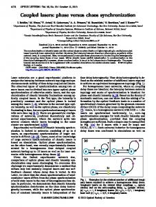
FIG. 2. Sketch of the neuron network, which in our simulations consist of a total of 50 neurons. Solid arrows mark the bidirectional electrical couplings, which are configured according to the WattsStrogatz algorithm. The dashed arrows mark the unidirectional chemical couplings, which are distributed randomly.

(2)

hci (t) =

N  j =1

γijc [ν − xi (t)]

1 , 1 + exp{−k[xj (t − τ ) − θ ]}

(3)

where ν represents the constant synaptic reversal potential. If ν > xi , we have what is called an excitatory coupling, and if ν < xi , it is inhibitory. This in an example of a so-called fast threshold modulation model, in which it is assumed that the synaptic dynamics works on a time scale much faster than the neuron interactions. Unlike the electrical synapses, the chemical synapses are allowed to be unidirectional. The results presented in this paper are taken from simulations performed on networks consisting of 50 neurons, where a total of 100 electrical couplings are configured according to the WattsStrogatz algorithm and where a total of 100 chemical couplings are chosen randomly over the set of ordered pairs (i,j ), as shown in Fig. 2. This is referred to here as the random net. We have also considered other more regular configurations, where the opposite extreme consisted of a ring of neurons with bidirectional electrical and chemical synapses between each pair of neighbors. In the latter case, the outcome was different. Based on the simulations, it appears as if the topology of the network determines the outcome mainly through the mean shortest path of the coupling graph composed of the union of e c the edge matrices γnm and γnm . This usually decreases with an increasing degree of randomness. Intermediate cases were also studied where the regular ring was taken as the starting point and subsequently a certain percentage of the couplings were rewired randomly. Through this procedure, one could see a gradual shift toward the results obtained for the random net. The iteration equations for the chaotic Rulkov model including

052903-2

BURSTING FREQUENCY VERSUS PHASE . . .

PHYSICAL REVIEW E 87, 052903 (2013) 1.5 1.0

T3

T2

0.5

T1

0 -0.5 -1.0 -1.5 -2.0 -2.5

FIG. 3. (Color online) Typical behavior of a Rulkov neuron interacting in a time-delayed network given by Eqs. (4). Parameter values are α = 4.15, μ = 0.003, x0 = −1.5, gc = 0.1, and ge = 0.1.

the interaction terms are thus given by α + yi (n) + ge hei + gc hci xi (n + 1) = 1 + xi2 (n) yi (n + 1) = yi (n) − μ[xi (n) − x0 ].

(4)

In our simulations, we fixed the parameter values to α = 4.15, μ = 0.003, x0 = −1.5, gc = 0.1, and ge = 0.1. In the sigmoid function for the delayed chemical coupling, we put k = 25 and θ = −1.4. The typical behavior of a single Rulkov neuron interacting in a network given by Eqs. (4) is shown in Fig. 3. The two measures discussed in this paper, the mean bursting frequency and the phase synchronization, both depend on the notion of burst. Assuming that the bursts are well defined, the bursting frequency of each individual neuron is defined as ωj = Bj /T ,

(5)

where Bj is the number of bursts of the j th neuron in the given time interval T . Thus, the mean bursting frequency  for the entire network is given by 1  = ωj . (6) N j In order to define the phase synchronization, we begin by introducing the phase for each neuron: ϕj (t) = 2π k + 2π

t− j tk+1

j tk j

− tk

.

(7)

j

Here, tk denotes the time of the beginning of the kth burst for the neuron with index j . The order parameter of the total phase synchronization is given by    T  N 1   iϕj (t)  (8) e r= . N T t=0  j =1  As can be seen from Fig. 3, for certain intervals there might be an ambiguity whether it should be considered as a single burst or composed of two or more bursts. We have resolved this by simply defining a burst as an interval of pulses that follows immediately after an interval, longer than or equal to a certain fixed length Tb , during which the neuron voltage stayed

5300

5500

5700

5900

6100

FIG. 4. (Color online) Illustration of the definition of burst of a Rulkov neuron through the characteristic interval Tb . If Tb < T2 , the interval in the figure counts as four bursts; if T2 < Tb < T1 , it counts as three bursts; and if T1 < Tb < T3 , it counts as two bursts.

below 0. For an illustration of this definition see Fig. 4. The length of this interval must be tuned for each set of parameters for it to produce the smoothest curves. In our simulations, we have taken Tb = 60. With this definition, the measures  and r are uniquely defined for the Rulkov model. An alternative way to define the bursts could be instead to identify the local maxima of the slow variable y, which is done, for example, in Refs. [17,18]. This, however, only shifts the problem of definition, since there are local maxima of y that do not correspond to clear pulses in the fast variable or appear to be intermediate between two “major” maxima. Our conclusion is that the definition based on the fast variable x, as described previously, is both sound and very easy to implement in a computer algorithm. The results of the simulations performed on a random net of 50 Rulkov neurons with inhibitory (ν = −2.5) and excitatory (ν = 1.5) chemical couplings are shown in Fig. 5. As can be seen, it looks as if the curves for  and r are almost mirror images of each other after the adjustment for a certain phase shift. III. INVESTIGATION ON A CONTINUOUS SYSTEM: THE HINDMARSH-ROSE MODEL

We will now demonstrate qualitatively similar results on a continuous neuron model, namely the Hindmarsh-Rose model. As mentioned in the introduction, the reason for doing this is to verify that the general behavior observed in Sec. II is not specific to the Rulkov model but holds more generally. The computations on the Hindmarsh-Rose model are much more expensive than on the Rulkov model, but one of the advantages with the former is that there is no problem identifying the beginning of each burst. The governing differential equations for the Hindmarsh-Rose model, including the same interaction terms and network configuration as before, are given by x˙i = yi + axi2 − xi3 − zi + I + ge hei + gc hci y˙i = 1 − dxi2 − yi z˙ i = μ[b(xi − x0 ) − zi ].

(9)

The Hindmarsh-Rose model is, just like the Rulkov model, capable of reproducing most of the interesting regimes of the

052903-3

´ NORDENFELT, USED, AND SANJUAN

PHYSICAL REVIEW E 87, 052903 (2013)

(a)Simulation on a random net of Rulkov neurons with inhibitory (ν = −2.5) chemical synapses

FIG. 6. (Color online) Typical behavior of the fast variable of a Hindmarsh-Rose neuron in a time-delayed network given by Eqs. (9). As can be seen, the beginning of each burst is very easy to identify. Parameter values are μ = 0.03, b = 4, d = 5, x0 = −1.6, a = 2.6, I = 4, gc = 0.1, ge = 0.1, k = 100, and θ = −0.25.

shown in Fig. 7. As can be seen, a similar pattern as was previously observed emerges. Although the shape of the curves are slightly different, the trends and relative position of the maxima and minima of  and r, respectively, are precisely the same as in the Rulkov model. IV. ANALYSIS USING THE KURAMOTO MODEL (b)Simulation on a random net of Rulkov neurons with excitatory (ν = 1.5) chemical synapses

FIG. 5. (Color online) (a) Simulation on a random net of Rulkov neurons with inhibitory (ν = −2.5) chemical synapses. (b) Simulation on a random net of Rulkov neurons with excitatory (ν = 1.5) chemical synapses. Average bursting frequency  (normalized to the zero time delay frequency) and phase synchronization r as a function of time delay obtained from computer simulations on a random net of 50 Rulkov neurons given by Eqs. (4). The parameter values were α = 4.15, μ = 0.003, x0 = −1.5, gc = 0.1, and ge = 0.1. The data presented is an average taken over 10 series of simulations with randomly chosen initial conditions.

observed neuron activity. Here we have three variables where x, as usual, represents the neuron voltage. The variable y is sometimes called the spiking variable and z the bursting variable. The latter two are also referred to as “gating” variables, since in the biological interpretation they govern the activation or inactivation of currents. Here it is z that operates on a slow time scale, whereas the pair (x,y) is viewed as the fast subsystem. Following Ref. [7], we have chosen as parameter values μ = 0.03, b = 4, d = 5, x0 = −1.6, a = 2.6, I = 4, gc = 0.1, and ge = 0.1. In the sigmoid function for the delayed chemical coupling, we put k = 100 and θ = −0.25. The typical behavior of a single Hindmarsh-Rose neuron is shown in Fig. 6. Obviously, in this case there is no problem identifying the beginning of each single burst, hence, the measures  and r are well defined and need no further clarification. The simulation results on a random net with inhibitory (ν = −1.5) and excitatory (ν = 1.5) chemical coupling, respectively, are

There are not many useful analytical tools for analyzing time-delayed dynamical systems. In order to gain further understanding, however, we will investigate two reduced models that could be viewed as variants of the well-known Kuramoto model. As will be seen, the curves for the average frequency and phase synchronization for these Kuramoto models resemble those obtained in previous sections on neuron networks with excitatory and inhibitory chemical synapses, respectively. A rigorous analysis connecting the Kuramoto models with the neuron networks is not in our possession and lies outside the scope of this paper. Nevertheless, the advantage with the time-delayed Kuramoto model is that, given some assumptions, an implicit functional relationship between the average frequency and the phase synchronization can be derived. The extent to which the insights gained from these formulas extrapolate to the time-delayed neuron networks is a matter of conjecture. Let each neuron be represented by a phase variable φi , which interacts with the other according to the following formula N  sin[φj (t − τ ) − φi (t)]. φ˙ i (t) = ω + N j =1

(10)

Here, ω is the natural frequency of the oscillators, is the coupling strength between the oscillators, τ is the time delay, and N is the number of oscillators. An analysis of this system was carried out in Ref. [22]. The average frequency is defined as

052903-4

N 1 ˙ ˙ (t) ≡ φ(t) ≡ φi (t). N i=1

(11)

BURSTING FREQUENCY VERSUS PHASE . . .

PHYSICAL REVIEW E 87, 052903 (2013)

a function of time delay but instead derive a formula relating the average frequency to the phase synchronization which, given the Ansatz Eq. (12), takes the form     N 1  iψj  (13) e r= . N  j =1  With the same assumption, Eq. (10) can now be expressed in the following way: =ω−

N  i(τ +ψi −ψj ) [e − e−i(τ +ψi −ψj ) ]. (14) 2iN j =1

If we do a summation over both indices i and j , we obtain

(a)Simulation on a random net of Hindmarsh-Rose neurons with inhibitory (ν = −1.5) chemical synapses

 = ω − r 2 sin(τ ),

(15)

which provides a relationship between the average frequency  and the phase synchronization r. Although Eq. (15) is only an implicit formula, there are some conclusions to be drawn. For weak coupling and moderate time delay (  1 and τ  1), the magnitude of the deviation in frequency from the natural frequency ω scales approximately with the synchronization squared. Moreover, the sign of the deviation varies periodically with the product of the time delay and the frequency. Numerical simulations that we performed reveal that the approximate validity of Eq. (15) holds also for geometries where, instead of having each neuron interacting with every other neuron, a smaller number of connections are chosen randomly. In Fig. 8 are the results of computer simulations performed on the system

(b)Simulation on a random net of Hindmarsh-Rose neurons with excitatory (ν = 1.5) chemical synapses

FIG. 7. (Color online) (a) Simulation on a random net of Hindmarsh-Rose neurons with inhibitory (ν = −1.5) chemical synapses. (b) Simulation on a random net of Hindmarsh-Rose neurons with excitatory (ν = 1.5) chemical synapses. Average bursting frequency  (normalized to the zero time delay frequency) and phase synchronization r as a function of time delay obtained from computer simulations on a random net of 50 Hindmarsh-Rose neurons given by Eqs. (9). The parameter values were μ = 0.03, b = 4, d = 5, x0 = −1.6, a = 2.6, I = 4, gc = 0.1, and ge = 0.1. The data presented is an average taken over 10 series of simulations with randomly chosen initial conditions.

φ˙ i (t) = ω + ij

N 

sin[φj (t − τ ) − φi (t)],

(16)

j =1

where N = 50, ω = 1, and the parameter ij takes the nonzero value 0.1 for a total of 200 pairs of indices (i,j ), half of which are chosen according to the Watts-Strogatz algorithm and half distributed randomly. On average, there are thus four couplings per neuron; hence, the “effective” coupling strength could

An analysis of the average oscillation frequency in similar systems was carried out by Zanette and Ko et al. [19–21]. By assuming that the phase variables reach a uniform synchronization frequency  and making the Ansatz φi (t) = t + ψi ,

(12)

with ψi independent of time, for certain regular network geometries they obtained closed analytical expressions for the synchronization frequency as a function of time delay. The shapes of some of these curves have a noteworthy similarity to those obtained in our simulations on Rulkov and HindmarshRose neurons. One of the weaknesses with the comparison, however, is that in those papers the phases ψi are given fixed values with the consequence that the phase synchronization is assumed to be independent of the time delay. Evidently this is not the case in the systems we have analyzed in previous sections. Here we will not derive formulas for the frequency as

FIG. 8. (Color online) Mean frequency  and phase synchronization r obtained from computer simulations on the time-delayed Kuramoto model given by Eqs. (16). The stars mark the value of the right-hand side of Eq. (15) (assuming = 0.4), taking the simulated values of  and r as parameters.

052903-5

´ NORDENFELT, USED, AND SANJUAN

PHYSICAL REVIEW E 87, 052903 (2013)

with the same parameter values as before but with the sine function replaced by a cosine. In this case, the relationship between the frequency and the synchronization corresponding to Eq. (15) reads  = ω + r 2 cos(τ ).

FIG. 9. (Color online) Mean frequency  and phase synchronization r obtained from computer simulations on the time-delayed Kuramoto model given by Eqs. (17). The stars mark the value of the right-hand side of Eq. (18) (assuming = 0.4), taking the simulated values of  and r as parameters.

be estimated as = 0.1 × 4 = 0.4. The curves obtained for the mean frequency and time-averaged phase synchronization display a significant (although imperfect) resemblance to those obtained previously on random nets with excitatory chemical synapses. We see that the synchronization gradually goes from an almost completely synchronized state to an almost incoherent state, while the frequency follows the characteristic curve seen previously. However, a notable difference shows up in the Rulkov model, where the synchronization recovers more quickly after the dip. In order to check how well the numerical results on the system Eqs. (16) fit the functional relationship Eq. (15), the simulated values of  and r were put into the right-hand side of Eq. (15) (assuming = 0.4) together with the corresponding time delay τ . The values obtained this way were then plotted as stars in the same graph as the curve for  [which would correspond to the left-hand side of Eq. (15)]. As can be seen, the simulated values fit Eq. (15) rather well, at least in the first part. If we now consider instead the system N 

(18)

Simulations on this system, which are shown in Fig. 9, reveal a behavior that resembles that obtained for the Rulkov and Hindmarsh-Rose networks with inhibitory chemical synapses. The choice of another trigonometric function phase-shifted in relation to the sine is not completely arbitrary if one considers the fact that, for the neuron networks, the curves in the case of excitatory couplings are almost identical to the second half of the curves for the networks with inhibitory synapses. In Fig. 9, the stars mark the values of the right-hand side of Eq. (18) (assuming = 0.4), taking the simulated values of  and r as parameters. We see that the simulated values fit Eq. (18) well. V. CONCLUSIONS

In this paper, we have studied, through numerical simulations, the mean bursting frequency and phase synchronization as a function of time delay on Rulkov and Hindmarsh-Rose neuron networks with time-delayed chemical synapses. We have found qualitatively similar results on both of these models. As an attempt to gain further insight, we have also studied time-delayed Kuramoto models that produced curves similar to those obtained on the Rulkov and Hindmarsh-Rose networks. For the Kuramoto models, we were able to derive analytical expressions for the relationship between the mean bursting frequency and the phase synchronization that agreed well with numerical simulation. These formulas state that, for weak coupling and moderate time delay (  1 and τ  1), the magnitude by which the average frequency is perturbed away from its value in the absence of time delay scales approximately with the square of the phase synchronization. This could explain the similarity in shape between the phase synchronization and the average frequency observed in certain intervals. ACKNOWLEDGMENT

(17)

Financial support from the Spanish Ministry of Science and Innovation under Project No. FIS2009-09898 is acknowledged.

[1] X. Liang, M. Tang, M. Dhamala, and Z. Liu, Phys. Rev. E 80, 066202 (2009). [2] Q. Wang, M. Perc, Z. Duan, and G. Chen, Phys. Rev. E 80, 026206 (2009). [3] Q. Wang, G. Chen, and M. Perc, PLoS ONE 6, e15851 (2011). [4] T. Perez, G. C. Garcia, V. M. Eguiluz, R. Vicente, G. Pipa, and C. Mirasso, PLoS ONE 6, e19900 (2011). [5] G. Tang, K. Xu, and L. Jiang, Phys. Rev. E 84, 046207 (2011). [6] I. Franovi´c and V. Miljkovi´c, Commun. Nonlinear Sci. Numer. Simulat. 16, 623 (2011).

[7] M. Jalili, Neurocomputing 74, 1551 (2011). [8] K. Iarosz, A. Batista, R. Viana, S. Lopes, I. Caldas, and T. Penna, Physica A 391, 819 (2012). [9] P. J. Uhlhaas and W. Singer, Neuron 52, 155 (2006). [10] A. Arenas, A. D´ıaz-Guilera, J. Kurths, Y. Moreno, and C. Zhou, Phys. Rep. 469, 93 (2008). [11] E. T. Rolls and A. Treves, Prog. Neurobiol. 95, 448 (2011). [12] M. I. Rabinovich, P. Varona, A. I. Selverston, and H. D. I. Abarbanel, Rev. Mod. Phys. 78, 1213 (2006).

φ˙ i (t) = ω + ij

cos[φj (t − τ ) − φi (t)],

j =1

052903-6

BURSTING FREQUENCY VERSUS PHASE . . .

PHYSICAL REVIEW E 87, 052903 (2013)

[13] B. Ibarz, J. M. Casado, and M. A. F. Sanju´an, Phys. Rep. 501, 1 (2011). [14] N. F. Rulkov, Phys. Rev. Lett. 86, 183 (2001). [15] D. C. Somers and N. Kopell, Biol. Cybern. 68, 393 (1993). [16] I. Belykh, E. de Lange, and M. Hasler, Phys. Rev. Lett. 94, 188101 (2005). [17] C. A. S. Batista, A. M. Batista, J. A. C. de Pontes, R. L. Viana, and S. R. Lopes, Phys. Rev. E 76, 016218 (2007).

[18] R. Viana, A. Batista, C. Batista, J. de Pontes, F. dos S. Silva, and S. Lopes, Commun. Nonlinear Sci. Numer. Simulat. 17, 2924 (2012). [19] D. H. Zanette, Phys. Rev. E 62, 3167 (2000). [20] T.-W. Ko, S.-O. Jeong, and H.-T. Moon, Phys. Rev. E 69, 056106 (2004). [21] T.-W. Ko and G. B. Ermentrout, Phys. Rev. E 76, 056206 (2007). [22] M. K. S. Yeung and S. H. Strogatz, Phys. Rev. Lett. 82, 648 (1999).

052903-7