Byte-Level Machine Reading across Morphologically Varied Languages

The Thirty-Second AAAI Conference on Artificial Intelligence (AAAI-18)

Byte-Level Machine Reading across Morphologically Varied Languages Tom Kenter∗

Llion Jones

Daniel Hewlett

University of Amsterdam Amsterdam The Netherlands

Google Research Mountain View United States

Google Mountain View United States

3

Abstract The machine reading task, where a computer reads a document and answers questions about it, is important in artificial intelligence research. Recently, many models have been proposed to address it. Word-level models, which have words as units of input and output, have proven to yield state-of-theart results when evaluated on English datasets. However, in morphologically richer languages, many more unique words exist than in English due to highly productive prefix and suffix mechanisms. This may set back word-level models, since vocabulary sizes too big to allow for efficient computing may have to be employed. Multiple alternative input granularities have been proposed to avoid large input vocabularies, such as morphemes, character n-grams, and bytes. Bytes are advantageous as they provide a universal encoding format across languages, and allow for a small vocabulary size, which, moreover, is identical for every input language. In this work, we investigate whether bytes are suitable as input units across morphologically varied languages. To test this, we introduce two large-scale machine reading datasets in morphologically rich languages, Turkish and Russian. We implement 4 byte-level models, representing the major types of machine reading models and introduce a new seq2seq variant, called encoder-transformer-decoder. We show that, for all languages considered, there are models reading bytes outperforming the current state-of-the-art word-level baseline. Moreover, the newly introduced encoder-transformer-decoder performs best on the morphologically most involved dataset, Turkish. The large-scale Turkish and Russian machine reading datasets are released to public.

1

3161

14636

1067

1628

-

В прошлом году Дмитрий работал нейрорадиологом. 15916

1211

1067

3

3161

14636

Чем занимался Дмитрий в прошлом году? -

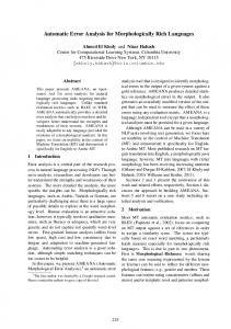
Нейрорадиолог Figure 1: Example from the Russian machine reading dataset. Document: Dmitry worked as neuroradiologist last year. Question: What was Dmitry’s occupation last year? Answer: Neuroradiologist. Numbers are positions in a frequency ordered vocabulary of over 950K words.

components like stemmers or parsers, yield state-of-the-art results (Cheng, Dong, and Lapata 2016; Hermann et al. 2015; Hewlett et al. 2016). An advantage of English in this context is its relatively limited morphology that allows word-based models to get a broad coverage of word types actively used, while maintaining a manageable vocabulary size. However, in morphologically richer languages, e.g., Turkish, Russian, Finnish and Czech, many more word types exist, due to highly productive prefix and suffix mechanisms, and even very large vocabularies cannot provide extensive coverage. To illustrate, Figure 1 shows a Russian example in which two forms of the word neuroradiologist do not appear in a vocabulary of over 950,000 most frequent words. In a setting like English, with less morphological transformations, a word-level model with a pointer mechanism (see, e.g., (Wang and Jiang 2017)), that can copy strings verbatim from the input to the output, would be able to reproduce the unknown word, but in this case doing so would lead to the incorrect answer. Answering this query is therefore impossible for a word-level model with a fixed vocabulary, even if it contains the 950,000 most frequent words. For a byte-level model, on the other hand, it is possible to reproduce the relevant word from the input and to apply the right morphological transformation, learned from similar training examples, even if the word itself was never observed during training. As another example, in Turkish, kolay means easy, kolaylas¸tırabiliriz means we can make it easier, while kolaylas¸tıramıyoruz means we cannot make it easier. Similarly, zor means hard or difficult, zorlas¸tırabiliriz means we can make it harder, while zorlas¸tıramıyoruz means we cannot make it harder. This illustrates that a lot of seman-

Introduction

Natural language understanding is one of the long-standing goals of artificial intelligence. It encompasses tasks like textual entailment (Rockt¨aschel et al. 2015), information extraction (Dong et al. 2014), semantic textual similarity (Kenter, Borisov, and de Rijke 2016), question answering (Fader, Zettlemoyer, and Etzioni 2013) and machine reading (Hermann et al. 2015). In this work we focus on the latter task of machine reading, where a machine reads a document and answers questions about it. On English machine reading tasks, neural word-level models, trained end-to-end without any additional NLP ∗

Work performed during an internship at Google Research. c 2018, Association for the Advancement of Artificial Copyright  Intelligence (www.aaai.org). All rights reserved.

5820

tic information is shared between words in Turkish, where in English separate words would be used. Hence, as in the Russian case, a larger vocabulary would be needed for Turkish compared to English to cover the same amount of text, which would increase the number of parameters of an embedding-based model dramatically. Learning these embeddings would, moreover, be hampered by fewer training examples being available per word type. To overcome the issues caused by a lack of vocabulary coverage and sparse training data as outlined above, models have been proposed that work at the sub-word level, e.g., morphemes (Luong, Socher, and Manning 2013; Botha and Blunsom 2014). Although morphemes are a natural unit for semantic composition, a drawback of these approaches is their dependency on high-quality morpheme segmentation algorithms, and the potential ambiguity of the morpheme segmentation itself. To avoid these complications, methods have been proposed that take characters as input (Zhang, Zhao, and LeCun 2015; Ling et al. 2015; Kim et al. 2016). An alternative approach is to consider bytes as input, which is appealing for a number of reasons. Firstly, bytes provide a universal encoding format across languages. As such, reading bytes ties in with a long-standing ambition to learn language from scratch (Zhang, Zhao, and LeCun 2015). Secondly, byte input allows for a small and fixed-size vocabulary of 256 tokens, which gives models a small memory footprint, compared to word-level models with tens or hundreds of thousands of words. A final advantage of using bytes over characters is that no character vocabulary has to be decided on (which can be non-trivial on real-world text like Wikipedia, where Chinese characters, or characters of any other alphabet, can appear in any given article). Having an identical vocabulary across languages makes for better model comparisons since there are fewer hyperparameters to choose (i.e., vocabularies and their sizes). It allows for an unbiased comparison of models, without introducing noise from a morphological decomposer. In short, the question we wish to answer in this research is: Is it advantageous, when processing morphologically rich languages, to use bytes rather than words as input and output in a machine reading task? Many different machine reading architectures have been proposed in literature (Hermann et al. 2015; Yang et al. 2016; Jozefowicz et al. 2016). Next to standard RNN sequence-to-sequence (seq2seq) models, convolutional RNNs (Zhang, Zhao, and LeCun 2015; Xiao and Cho 2016), word-character hybrid models (Luong and Manning 2016) and memory networks (Weston, Chopra, and Bordes 2015; Miller et al. 2016; Sukhbaatar et al. 2015; Kenter and de Rijke 2017) have been proposed1 . We implement 4 byte-level models, based on these families of models, and present a new seq2seq variant, called encodertransformer-decoder. We evaluate all models on three large datasets: an already existing English dataset, and two ad-

ditional datasets in Turkish and Russian, created specifically for this purpose. The two additional datasets are publicly available at http://goo.gl/wikireading. We compare results to the strongest word-level model available, and show that reading byte-level input is beneficial for all three languages considered. Our main contributions are: • We implement 4 byte-level models based on the major families of machine reading models (vanilla RNN, convolutional RNN, hybrid word-byte-level, memory networks) and propose a seq2seq network variant, called encodertransformer-decoder. It is the first time, to our knowledge, that multiple byte-level models are systematically compared on a single machine reading task, across fundamentally different languages. • We provide a platform for comparing machine reading models across different types of languages, by releasing 2 large machine reading datasets, one in Turkish, one in Russian — next to the already existing one in English. • We show that for all three languages considered in the experiments, there are models reading bytes outperforming the current state-of-the-art word-level model. We describe the datasets we introduce in §2. To allow for an in-depth discussion of existing research related to our work, we first describe the models we use in §3, experiments in §4, and results and analysis in §5 and §6, before we discuss related work in §7. We conclude in §8.

2

Datasets and problem motivation

In (Hewlett et al. 2016) an English reading comprehension dataset is presented, called WikiReading. The set is constructed from Wikipedia and Wikidata (Vrandeˇci´c and Kr¨otzsch 2014) by constructing (document, property, value) triples, where the property and value originate from Wikidata triples, and the document is the original Wikipedia article text, as linked to in Wikidata. This process yields a challenging dataset as, unlike in other datasets, e.g., WikiQA (Yang, tau Yih, and Meek 2015), the values in the triples are not necessarily present in the Wikipedia document verbatim, and may have to be inferred from the text. In the experiments the property and document are provided as input to a reading comprehension algorithm, where the property is interpreted as being a query about the document, to which the value is the correct answer. For the experiments on Russian and Turkish, we construct new datasets following the procedure described above. The size of every dataset is proportional to the size of the Wikipedia per language. The already existing English dataset is split in training/validation/test according to a 85/10/5 distribution. For the new sets, which are smaller, we choose a 80/10/10 split, to keep enough examples in the test set. Table 1 presents an overview of the number of examples (i.e., triples) for each dataset, where we list the numbers for the English dataset too for comparison. The sets are publicly available.2

1 Fully convolutional models for encoding textual data have been proposed (Zhang, Zhao, and LeCun 2015) in text classification settings. Their performance in domains other than classification is not evident and we do not consider them in our experiments.

2 The Turkish and Russian datasets can be downloaded from http://goo.gl/wikireading.

5821

applied, at every time step t, the hidden state ht of a re¯ t , an new version of ht augcurrent cell is replaced by h mented by attention. Following, e.g., (Vinyals et al. 2015; ¯ t as: Luong and Manning 2016) we compute h

Table 1: Number of examples per dataset. The bottom part lists the percentage of answers appearing verbatim in the document and the percentage of out-of-vocabulary tokens in the documents. English

Turkish

Russian

16.0M 1.89M 941K

655K 81.6K 82.6K

4.26M 531K 533K

67.8 3.70

52.3 7.51

55.9 9.78

training validation test % verbatim % OOV tokens

at dt ¯t h

3.2

ati hia

(2) (3)

=

tanh(W · dt ||ht ),

(4)

Encoders

Below we describe the encoder modules used in our experiments in §4. Multi-level and bidirectional RNNs The default way of encoding input in a sequence-to-sequence setup is to use an RNN. We test two commonly used variants, multi-level RNNs and bi-directional RNNs. The multi-level RNN (Sutskever, Vinyals, and Le 2014; Cho et al. 2014), referred to as Deep Reader in (Hermann et al. 2015), is an extension of a single-layer RNN encoder. Instead of having one recurrent cell, multiple cells are stacked and a separate set of parameters is maintained at every level. At level i, Equation 1 becomes θit = f (¯ xti , θit−1 ), where the t t t t input x ¯0 = x and x ¯i = hi−1 for i > 0. I.e., at every level but the first one, the input is replaced by the hidden state at the previous level. The multi-layer RNN encoder is illustrated in Figure 2a. Bidirectional RNNs (Figure 2b) have proven to be a robust choice in many different settings (Ling et al. 2015; Hermann et al. 2015). The bidirectional RNN employs two multi-level encoders as described above: one reading the input from left to right, and one reading it from right to left. → − ← − They yield two final states, ht and ht , respectively. Following, e.g., (Hermann et al. 2015), we concatenate the two states to get the final state of the two encoders combined: → − ← − ht = ht  ht , which we project down to the original state → − ← − size when appropriate: ht = Wprojection · ht  ht .

Models

Preliminaries

Cells At the heart of every sequence encoder is a recurrent cell, which reads input symbol by symbol, while maintaining a number of internal parameters at every time step. At time step t, new values for the internal parameters θt are computed from a representation of an input symbol, xt , and the current values of the internal parameters θt−1 : θt = f (xt , θt−1 )

I 

where Ha are the states to attend over, typically Hencoder , hia is the state in Ha at position i, W is an extra trainable parameter, and || denotes concatenation.

Next to our baseline, we consider 5 encoder-decoder models (Kalchbrenner and Blunsom 2013; Sutskever, Vinyals, and Le 2014; Cho et al. 2014) in our experiments. We note that in the present setting of machine reading, rather than having a single input string, we have two, a question and a document. The key focus of our experiments is to distinguish between different ways of encoding the question and documents. Therefore, we apply a generic setup, where the encoder varies, while the decoder is the same for every model. As some building blocks are shared between models, we first discuss preliminaries in §3.1. The encoder models are detailed in §3.2 and the decoder model in §3.3.

3.1

=

sof tmax(ht · Ha )

i=1

The bottom part of Table 1 indicates how the datasets differ in character. In the morphologically rich languages, only approximately half of the answers appear in the documents. Furthermore, the documents in these languages contain up to three times as many out-of-vocabulary words as the documents in the English dataset. These numbers motivate exploring models that do not rely on word-level input only.

3

=

Hybrid word-byte As argued in §1, in morphologically rich languages many words might not appear in the vocabulary. An alternative to treating the input as either a stream of words or bytes is a hybrid approach, where the input is read word by word, and the model can resort to byte-level reading when a word is out-of-vocabulary. The word-byte hybrid model we employ follows the model presented in (Luong and Manning 2016), specifically, the separate-path variant. Every time a word is encountered that does not appear in the word vocabulary, a byte-level encoder is run, whose last hidden state is used as distributed representation of the word. As the recurrent cells following this initial layer are unaware of the source of a word representation (i.e., a word embedding matrix, or a byte-level encoder), the byte-level encoder learns to map words to the same embedding space

(1)

For function f , we experiment with both LSTM and GRU cells, as both are frequently used in literature without one consistently outperforming the other across models and tasks. Our LSTM implementation follows (Sak, Senior, and Beaufays 2014; Ling et al. 2015), while the GRU implementation follows (Cho et al. 2014). Attention To give the decoder more information about the input, an attention mechanism was proposed in (Bahdanau, Cho, and Bengio 2014), where the decoder has access to the hidden states of the encoder. One of the parameters in θ in Equation 1 as maintained both in a GRU and LSTM cell is a hidden state h. When the attention mechanism is

5822

o

o

u

u

t

ans1 ans2

t

p



n

o

i

u

t





i

n

wrd1

p i

(a) Multi-level RNN

n

u

p

(b) Bidirectional RNN o

u

n

wrd2 k

(c) Hybrid word-byte model o

t

u

t

i

s t

u p

n n

t





p

u

q

u

e

u p

d

(d) Convolutional-recurrent

o

c

(e) Memory network/encoder-transformer-decoder

Figure 2: Graphical illustration of the models employed (best viewed in color). The attention mechanism of the decoder, which is employed for all models, is left out for clarity. the word vocabulary uses. At decoding time a similar procedure is employed, where a word-level decoder produces output, and a separate byte-level decoder is resorted to when a special ‘unknown word’ token is encountered. A graphical illustration of this model is provided in Figure 2c.

the final state of the question encoder. Specifically, at every time step, a recurrent cell attends over the hidden states of the document encoder, and is provided with the final state of the question encoder as input (i.e., it has the same input at every time step). That is xt in Equation 1 is hnquestion , the last hidden state of the question encoder, for a query of length n. The states to attend over for the memory module, Ha in Equation 2, are Hdocument , the hidden states of the document encoder. Finally, a crucial part of the memory network architecture is that the attention of the decoder is on the memory states. Figure 2e shows a graphical illustration of the memory network. The attention of the memory cells is represented by grey dashed lines.

Convolutional-recurrent The convolutional-recurrent model is based on the model in (Xiao and Cho 2016). Convolutional filters are applied to the input byte embeddings, or directly to one-hot encodings. After multiple levels of convolutions a max-pooling layer is applied. This gives a fixed-size vector with as many elements as there are convolutional filters. Multiple of these fixed-size vectors are obtained from the input, the exact number depending on the input size, the receptive field of the convolutions (the window of input symbols they observe) and the stride. Each of these vectors is a distributed representation of a window of input symbols. A recurrent encoder is used to encode this sequence of representations into its final state. Figure 2d provides a graphical representation of this model. An alternative approach, further discussed in §7, is to take word boundaries into account (Jozefowicz et al. 2016). Preliminary experiments showed inferior performance and we leave this variant out of our experiments.

Encoder-transformer-decoder We present a variant of the memory network architecture, which differs in that the decoder attends over the document encoder states. Although this is a small deviation in terms of architecture, the model in fact now learns something crucially different. Where, in the memory network scenario, the memory cells can copy parts of the input document based on the question, in the new setup, the internal states of the intermediate RNN do not serve as memories, because the decoder is in fact agnostic to them. Rather, the function of the intermediate RNN is to optimize the final state of the document encoder for the decoder, with respect to the question. As this model is similar to, but different from, the recently proposed encoderreviewer-decoder model (Yang et al. 2016), we refer to it as encoder-transformer-decoder model. Since the key difference between this model and the memory model is in the attention of the decoder, which is not depicted in Figure 2, the graphical depiction of these models is shared in Figure 2e.

Memory networks There are two main differences between memory networks (Weston, Chopra, and Bordes 2015; Miller et al. 2016; Sukhbaatar et al. 2015; Kenter and de Rijke 2017) and the standard encoder-decoder architecture: 1) a number of recurrent steps is performed between encoding and decoding 2) there are two separate input encoders — one for the question and one for the document. The final state of the document encoder, before being presented to the decoder, is modified during a number of recurrent steps (also referred to as memory hops), conditioned on

See §7 for a discussion of differences and similarities between the models presented here and existing models.

5823

Table 4: Results for multi-level RNN (RNN), bidirectional RNN (Bidir), convolutional RNN (Conv-rnn), hybrid wordbyte (Word-byte), memory network (Memory) and encodertransformer-decoder (Enc-trans-dec).

Table 2: Hyperparameter values tuned over Embedding size Internal state size Number of RNN cells stacked RNN cell type Input/output embedding tying Gradient clipping Learning rate

128/256 256/512 1/2 LSTM/GRU yes/no 0.1/1 10-5 /10-4 /10-3

Table 3: Filter and maxpool width per layer for the convolutional RNN. For additional details, see (Xiao and Cho 2016). # layers

Filter width

maxpool width

2 3 4 5

5, 3 5, 5, 3 5, 5, 3, 3 5, 5, 3, 3, 3

2, 2 2, 2, 2 2, 2, 2, 2 2, 2, 2, -, 2

C2R1 C3R1 C4R1 C5R1

3.3

Russian

English

RNN Bidir Conv-rnn Word-byte Memory Enc-trans-dec

0.6956 0.6627 0.5753 0.6654 0.6899 0.6956

0.5784 0.5431 0.4123 0.5874 0.5612 0.5808

0.7176 0.6615 0.5364 0.7418 0.7176 0.7182

Word-level

0.6365

0.5759

0.7365

maximum number of output steps is 50, which is enough for all answers in the training and validation set. Table 3 lists the additional hyperparameters tuned over for the convolutionalrecurrent model. All models are trained with stochastic gradient descent. The learning rate is adapted per parameter with Adam (Kingma and Ba 2015). Batch size is 64. After every 50,000 batches, the learning rate is divided by 2. Baseline model We compare the performance of our bytelevel models to the model performing strongest on the English dataset in (Hewlett et al. 2016), which is a word-level sequence-to-sequence model with LSTM cells with state size 1024, a word vocabulary of 100,000, and 300d embeddings. The model employs placeholders to handle outof-vocabulary words. To keep comparison between models as clean as possible, we do not pre-train the embeddings as in (Hewlett et al. 2016). Evaluation An answer is considered to be correct if it is exactly the same as the ground truth answer (there is no stemming and no normalization, except for dates, which were all converted to one format, like 1 January 1970). As some questions have a set of values as an answer (e.g., Children of person X), we compute precision and recall for every example and use the mean F1 over all examples as evaluation metric, following (Hewlett et al. 2016).

Decoder

Except for the word-byte hybrid model, we use the same decoder for all models, a single level RNN. At every time step a softmax over the byte vocabulary is computed, and cross entropy loss is calculated. The decoder always applies attention to the hidden states of the document encoder, except for the memory model, where it attends over the hidden states of the memory cells (§3.2). In all experiments, when an LSTM cell is used in the encoder, an LSTM cell is used in the decoder, and likewise for GRUs.

4

Turkish

Experimental setup

Table 2 lists the values of hyperparameters tuned over on the validation data. For the multi-level, bidirectional and convolutional-recurrent encoder, the document is appended to the query with a separator symbol in between. All embeddings are trained from scratch (i.e., no pre-trained vectors are used). We experiment with either sharing input and output embeddings, i.e., a single embedding matrix is employed, or having two separate embedding matrices (Press and Wolf 2016). For the memory network and the encodertransformer-decoder model, the intermediate RNN performs 2 recurrent steps, as this yielded consistent performance in preliminary experiments. At most 50 bytes are read of each question, which is sufficient because questions are rarely longer than this. At most 400 bytes are read from the documents. This limit is imposed by resources — memory usage becomes an issue when we unroll the RNNs longer for. We note that the fact that 400 bytes is enough to answer the questions in our dataset may be due to Wikipedia being structured the way it is, i.e. the first paragraph of a Wikipedia page is usually very informative. The word-byte hybrid model observes roughly the same amount of input: 60 words per document, which, given the average word length in English, is ∼ 400 characters. The other languages have longer words, so this model might have the advantage of reading slightly more input on average. The

5

Results

Table 4 lists the main results of the experiments. The first observation from the results is that for every language, there is a model reading bytes that outperforms the word-level baseline. Interestingly, there are differences between models across datasets which can be explained by the characteristics of the languages in the dataset. On the dataset of the morphologically most involved language we consider, Turkish, the difference between bytelevel and word-level models is most pronounced. Here, we use diversity of word forms found in a given amount of text as a proxy for measuring morphological complexity. The ratio of unique word forms to total tokens illustrates the difference between languages ((number of types) / (number of tokens), numbers × 1000 for clarity): 1.1 for English, 2.9 for Russian, and 8.1 for Turkish. On the Turkish dataset, all

5824

Table 5: Results per query type Categorical Turkish Russian English

Relational Turkish Russian English

RNN Bidir Conv-rnn Word-byte Memory Enc-trans-dec

0.8528 0.8420 0.8059 0.8478 0.8576 0.8539

0.7388 0.7289 0.7082 0.8022 0.7369 0.7427

0.8482 0.8332 0.7794 0.8656 0.8595 0.8461

0.5453 0.4906 0.3539 0.4903 0.5290 0.5437

0.4080 0.3524 0.1206 0.3833 0.3769 0.4089

0.5752 0.4594 0.2385 0.5824 0.5561 0.5749

0.7796 0.7658 0.4857 0.6784 0.7740 0.7822

0.7253 0.7142 0.1039 0.7507 0.7147 0.7276

0.8075 0.7984 0.3891 0.8000 0.8067 0.8093

Word-level

0.8125

0.7513

0.8531

0.4676

0.4019

0.5875

0.6218

0.7305

0.8021

byte-level models outperform the word-level model, except for the convolutional RNN. This result seems to corroborate the hypothesis stated in §1, that a word-level model has trouble getting enough coverage in this language. The word-byte hybrid model lags behind on the Turkish data, compared to the other datasets. This is likely to be caused by the larger number of unknown words in the Turkish dataset (cf. Table 1). In English, copying words from the input document works, as demonstrated already by the word-level placeholder model being the best performer reported in (Hewlett et al. 2016). This indicates that the unknown words might be, e.g., names and proper nouns, occurring in the text. In Turkish, however, due to the morphological richness, many more words, not just proper nouns, are out-of-vocabulary, but there is relatively little data per word to learn from. Russian, being highly inflective rather than agglutinative like Turkish, has a lower ratio of word forms over word tokens. This is reflected in the results, where only two bytelevel models outperform the word-level model, and only marginally. The encoder-transformer-decoder model, while not the top performer, does beat the word-level baseline. We should note that, although the improvements of the byte-level models over the word-level models seem small, the model sizes of the byte-only models are considerably smaller, as they have a vocabulary of 256 rather than 100,000. As such, the strongest byte-only model across the datasets of morphologically rich languages, the encodertransformer-decoder model, yields two crucial benefits over the word-level baseline — the model performing best on the English dataset in (Hewlett et al. 2016): 1) improved performance 2) while having a substantially smaller memory footprint. This result leads us to answer our research question “Is it advantageous, when processing morphologically rich languages, to use bytes rather than words as input and output in a machine reading task?” affirmatively. Finally, on the English data, we do not expect the bytelevel models to have an advantage over the word-level model, which is confirmed by the results in Table 4. The exception to this rule is the word-byte hybrid model. Most notably, not only does it outperform the word-level model in Table 4 — which has access to 60 words — it also outperforms the best performing model as reported in (Hewlett et al. 2016) which reads 300 words, and has a score of 0.718. This shows that having access to more information might

Dates Turkish Russian English

actually hamper a model. More importantly, it indicates that reverting to reading bytes is a better way of dealing with out-of-vocabulary words than using placeholders. There are multiple unexpected results in Table 4. Most remarkably, bidirectional models do not perform better than uni-directional RNNs. This is a surprising deviation from previous research, which has shown them to be consistent performers. The results indicate that on the byte-level, an extra backward pass does not yield additional, complementary information. Next, it is not clear from scrutiny of the data, why the scores on the Russian data should be lower in general (roughly 10-15% for each model). Additional analysis is necessary to disclose the underlying reason. To sum up, the results show that byte-level input is beneficial for all three language considered. It is interesting to see that the advantage of reading bytes versus words appears to be proportional to morphological complexity of the language involved. On the English dataset, only one byte-level model outperforms the word-level baseline — the best scoring model in (Hewlett et al. 2016). On the dataset of the inflective language, Russian, multiple byte-level models improve over the baseline, while on the data for the agglutinative language, Turkish, all but one do.

6

Analysis

Results per query type Some properties, like gender or instance of are category-like, while some, like mayor, are more open-ended. We split out the results in Table 4 per query type in Table 5. We distinguish between categorical (few possible answers) and relational (a large set of possible answers). As dates are notoriously hard to deal with, we also split out a separate date category. A key observation from Table 5 is that the encodertransformer-decoder model is a consistent (near) top performer across categories. Interestingly, on the Turkish dataset, the most pronounced difference between the well performing byte-level models and the word-level model is in the hardest category, the relational queries. Visualization of encoder-transformer-decoder network As noted above, the encoder-transformer-decoder model is a top or near top performer on both morphologically rich languages. To gain insight in its inner workings, we visualize its attention vectors for two examples, in Figure 3. For ease of understanding, the examples are from the English

5825

J a u me J a u me J a u me J a u me J a u me

Bu s q u e t s Bu s q u e t s Bu s q u e t s Bu s q u e t s Bu s q u e t s

i i i i i

Mo l l e r a Mo l l e r a Mo l l e r a Mo l l e r a Mo l l e r a

( Gi r o n a , ( Gi r o n a , ( Gi r o n a , ( Gi r o n a , ( Gi r o n a ,

19 0 4 19 0 4 19 0 4 19 0 4 19 0 4

-

Ba r c e l o n a , Ba r c e l o n a , Ba r c e l o n a , Ba r c e l o n a , Ba r c e l o n a ,

19 6 8 ) 19 6 8 ) 19 6 8 ) 19 6 8 ) 19 6 8 )

wa s wa s wa s wa s wa s

a a a a a

Ca t a l a n Ca t a l a n Ca t a l a n Ca t a l a n Ca t a l a n

sc ul pt or sc ul pt or sc ul pt or sc ul pt or sc ul pt or

and and and and and

pai nt er pai nt er pai nt er pai nt er pai nt er

of of of of of

t he t he t he t he t he

n o u c e n t i s me n o u c e n t i s me n o u c e n t i s me n o u c e n t i s me n o u c e n t i s me

gener at i on. gener at i on. gener at i on. gener at i on. gener at i on.

He He He He He

wa s wa s wa s wa s wa s

(a) Question: instance of. Ground truth: human. Prediction: human Un i v e r s i t y i s a s t o p o n t h e No r t h w e s t L i n e ( Ro u t e 2 0 1) o f t h e CT r a i n l i g h t r a i l s y s t e m i n Ca l g a r y , A l b e r t a . T h e s t a t i o n Un i v e r s i t y i s a s t o p o n t h e No r t h w e s t L i n e ( Ro u t e 2 0 1) o f t h e CT r a i n l i g h t r a i l s y s t e m i n Ca l g a r y , A l b e r t a . T h e s t a t i o n Un i v e r s i t y i s a s t o p o n t h e No r t h w e s t L i n e ( Ro u t e 2 0 1) o f t h e CT r a i n l i g h t r a i l s y s t e m i n Ca l g a r y , A l b e r t a . T h e s t a t i o n Un i v e r s i t y i s a s t o p o n t h e No r t h w e s t L i n e ( Ro u t e 2 0 1) o f t h e CT r a i n l i g h t r a i l s y s t e m i n Ca l g a r y , A l b e r t a . T h e s t a t i o n Un i v e r s i t y i s a s t o p o n t h e No r t h w e s t L i n e ( Ro u t e 2 0 1) o f t h e CT r a i n l i g h t r a i l s y s t e m i n Ca l g a r y , A l b e r t a . T h e s t a t i o n

(b) Question: country. Ground truth: Canada. Prediction: Canada

Figure 3: Visualization of attention vectors of encoder-transformer-decoder model. Attention over the relevant part of the input is displayed for the 2 intermediate RNN steps (first 2 lines) and the decoder steps (next 50 lines, of which only the first 3 are shown for brevity). al. 2015) an embedding approach is used to represent the input and generate output, while in our setting RNNs are used at both stages for better comparison to the other models. In (Kenter and de Rijke 2017) a hierarchical input reader is proposed, which reads words into sentences, and transforms sentence embeddings to memory, a setting we did not try in our experiments.. The memory network we employ is related to the reader network described in (Hermann et al. 2015) and much like the encoder-reviewer-decoder model in (Yang et al. 2016), where a reviewer module is applied between encoding and decoding. A difference is that our models repeatedly attend over the document conditioned on the question, while in (Hermann et al. 2015) attention is performed once. The encoder-transformer-decoder is related to the encoder-reviewer-decoder network in (Yang et al. 2016). There are multiple differences between the two models. The encoder-transformer-decoder model has a separate question encoder, which is absent from the encoder-reviewerdecoder model. More importantly, however, the decoder of the encoder-transformer-decoder model attends over the document encoder states, rather than over the reviewer states. Lastly, in (Yang et al. 2016) experiments are run with discriminative supervision for the reviewer model at training time, a setting we do not use on our experiments in §4.

dataset. Note that, since the inputs are bytes, the attention is typically at the end of a word (when all the bytes of a word have been read). In Figure 3a, the answer does not appear in the document but has to be inferred. The first transformer step focuses on words indicating a human actor, like sculptor, painter and he. Figure 3b shows an example of the first transformer step solving the answer completely. The attention is on Calgary, Alberta which is enough, apparently, to infer the corresponding country. In both cases, the intermediate RNN steps, by focusing on the crucial parts of the input and altering their internal state accordingly, appear to provide the decoder with all the information it needs to generate the answer, which results in the decoder attention being very weak. Hyperparameters As to the hyperparameters tuned over (Table 2) some patterns could be discerned. Most notably, GRUs proved to be better than LSTMs in the majority of cases. The learning rate is a crucial factor, which is less surprising. Tying the input and output embeddings typically helped. Embedding and state sizes did not matter greatly, nor did the various values for gradient clipping.

7

Related work

Byte- and character-level models have been used in settings such as classification (Zhang, Zhao, and LeCun 2015), NER and POS tagging (Gillick et al. 2016), and language modeling (Kim et al. 2016), also on morphologically rich languages (Ling et al. 2015; Chung, Cho, and Bengio 2016). A word-based variant of the convolutional-recurrent model we use is proposed in (Jozefowicz et al. 2016). The key difference is that the receptive window of the convolutions in the model we use ranges over the entire input sequence, and hence can cross word boundaries, while in the model of (Jozefowicz et al. 2016), the convolutions can only see single words. Preliminary experiments showed worse performance for the word-level convolution model, and hence we left it out of our main experiments. The memory network we implement is based on the work in (Weston, Chopra, and Bordes 2015; Sukhbaatar et al. 2015; Kenter and de Rijke 2017; Yang et al. 2016). However, in (Weston, Chopra, and Bordes 2015; Sukhbaatar et

8

Conclusion

We introduced two large-scale machine reading datasets of morphologically rich languages, Turkish and Russian, which we publicly release. The new datasets, together with the English dataset published previously, provide a unique collection for comparing machine reading algorithms on one task, across principally different languages. We provide results for byte-level implementations of four major architectures of machine reading models. Furthermore, we introduce an encoder-transformer-decoder network model that performs best on Turkish data, and is competitive on the Russian data. It is the first time, to our knowledge, that multiple byte-level models are systematically compared on a single machine reading task, across fundamentally different languages. We show that on all datasets, reading input at byte level is ben-

5826

eficial, and that the encoder-transformer-decoder model is top or near top performer on the morphologically more involved languages. It is interesting to see that the advantage of reading bytes versus words seems to be proportional to the morphological complexity of the languages considered, as pointed out in §5. More research is needed to confirm whether this trend holds more broadly. We hope that the new datasets encourage the development of novel approaches for machine reading in morphologically rich languages, especially since the results on the datasets in these languages are still considerably lower than on the English counterpart.

9

Kenter, T.; Borisov, A.; and de Rijke, M. 2016. Siamese CBOW: Optimizing word embeddings for sentence representations. In Proceedings of the The 54th Annual Meeting of the Association for Computational Linguistics (ACL 2016), 941–951. Kim, Y.; Jernite, Y.; Sontag, D.; and Rush, A. M. 2016. Characteraware neural language models. In AAAI. Kingma, D., and Ba, J. 2015. Adam: A method for stochastic optimization. In The International Conference on Learning Representations (ICLR). Ling, W.; Lu´ıs, T.; Marujo, L.; Astudillo, R. F.; Amir, S.; Dyer, C.; Black, A. W.; and Trancoso, I. 2015. Finding function in form: Compositional character models for open vocabulary word representation. In EMNLP. Luong, M.-T., and Manning, C. D. 2016. Achieving open vocabulary neural machine translation with hybrid word-character models. In ACL. Luong, T.; Socher, R.; and Manning, C. D. 2013. Better word representations with recursive neural networks for morphology. In CoNLL. Miller, A.; Fisch, A.; Dodge, J.; Karimi, A.-H.; Bordes, A.; and Weston, J. 2016. Key-value memory networks for directly reading documents. In EMNLP. Press, O., and Wolf, L. 2016. Using the output embedding to improve language models. arXiv preprint arXiv:1608.05859. Rockt¨aschel, T.; Grefenstette, E.; Hermann, K. M.; Koˇcisk`y, T.; and Blunsom, P. 2015. Reasoning about entailment with neural attention. In ICLR. Sak, H.; Senior, A. W.; and Beaufays, F. 2014. Long shortterm memory recurrent neural network architectures for large scale acoustic modeling. In INTERSPEECH. Sukhbaatar, S.; Szlam, A.; Weston, J.; and Fergus, R. 2015. Endto-end memory networks. In NIPS. Sutskever, I.; Vinyals, O.; and Le, Q. V. 2014. Sequence to sequence learning with neural networks. In NIPS. Vinyals, O.; Kaiser, Ł.; Koo, T.; Petrov, S.; Sutskever, I.; and Hinton, G. 2015. Grammar as a foreign language. In NIPS 2015. Vrandeˇci´c, D., and Kr¨otzsch, M. 2014. Wikidata: a free collaborative knowledgebase. Communications of the ACM 57(10):78–85. Wang, S., and Jiang, J. 2017. Machine comprehension using match-LSTM and answer pointer. In ICLR. Weston, J.; Chopra, S.; and Bordes, A. 2015. Memory networks. In ICLR. Xiao, Y., and Cho, K. 2016. Efficient character-level document classification by combining convolution and recurrent layers. arXiv preprint arXiv:1602.00367. Yang, Z.; Yuan, Y.; Wu, Y.; Salakhutdinov, R.; and Cohen, W. W. 2016. Encode, review, and decode: Reviewer module for caption generation. In NIPS. Yang, Y.; tau Yih, W.; and Meek, C. 2015. WikiQA: A challenge dataset for open-domain question answering. In EMNLP. Zhang, X.; Zhao, J.; and LeCun, Y. 2015. Character-level convolutional networks for text classification. In Advances in Neural Information Processing Systems, 649–657.

Acknowledgments

The authors wish to express their gratitude to their colleagues in Google Research for their help. In particular, thanks to Tom Schumm for his help with the hybrid model, Thyago Duque for his help with the convolutional models and Illia Polosukhin for general advise. Additionally, many thanks to Dilek Onal for her help with Turkish examples, and Alexey Borisov for his help with the Russian examples.

References Bahdanau, D.; Cho, K.; and Bengio, Y. 2014. Neural machine translation by jointly learning to align and translate. In ICLR 2015. Botha, J. A., and Blunsom, P. 2014. Compositional morphology for word representations and language modelling. In ICML. Cheng, J.; Dong, L.; and Lapata, M. 2016. Long short-term memory-networks for machine reading. In EMNLP. Cho, K.; Van Merri¨enboer, B.; Gulcehre, C.; Bahdanau, D.; Bougares, F.; Schwenk, H.; and Bengio, Y. 2014. Learning phrase representations using RNN encoder-decoder for statistical machine translation. In EMNLP. Chung, J.; Cho, K.; and Bengio, Y. 2016. A character-level decoder without explicit segmentation for neural machine translation. In ACL. Dong, X.; Gabrilovich, E.; Heitz, G.; Horn, W.; Lao, N.; Murphy, K.; Strohmann, T.; Sun, S.; and Zhang, W. 2014. Knowledge Vault: a web-scale approach to probabilistic knowledge fusion. In KDD. Fader, A.; Zettlemoyer, L. S.; and Etzioni, O. 2013. Paraphrasedriven learning for open question answering. In ACL. Gillick, D.; Brunk, C.; Vinyals, O.; and Subramanya, A. 2016. Multilingual language processing from bytes. In NAACL-HLT. Hermann, K. M.; Kocisky, T.; Grefenstette, E.; Espeholt, L.; Kay, W.; Suleyman, M.; and Blunsom, P. 2015. Teaching machines to read and comprehend. In NIPS. Hewlett, D.; Lacoste, A.; Jones, L.; Polosukhin, I.; Fandrianto, A.; Han, J.; Kelcey, M.; and Berthelot, D. 2016. WIKIREADING: A novel large-scale language understanding task over wikipedia. In ACL 2016. Jozefowicz, R.; Vinyals, O.; Schuster, M.; Shazeer, N.; and Wu, Y. 2016. Exploring the limits of language modeling. arXiv preprint arXiv:1602.02410. Kalchbrenner, N., and Blunsom, P. 2013. Recurrent continuous translation models. In EMNLP. Kenter, T., and de Rijke, M. 2017. Attentive memory networks: Efficient machine reading for conversational search. In CAIR’17 at SIGIR 2017.

5827