SSV 2008
Symbolic and Abstract Interpretation for C/C++ Programs Helge L¨oding2 ,4 GESy Graduate School of Embedded Systems University of Bremen and Verified Systems International GmbH Germany
Jan Peleska1 ,3 Centre of Information Technology University of Bremen Germany
Abstract We present a construction technique for abstract interpretations which is generic in the choice of data abstractions. The technique is specialised on C/C++ code, internally represented by the GIMPLE control flow graph as generated by the gcc compiler. The generic interpreter handles program transitions in a symbolic way, while recording a history of symbolic memory valuations. An abstract interpreter is instantiated by selecting appropriate lattices for the data types under consideration. This selection induces an instance of the generic transition relation. All resulting abstract interpretations can handle pointer arithmetic, type casts, unions and the aliasing problems involved. It is illustrated how switching between abstractions can improve the efficiency of the verification process. The concepts described in this paper are implemented in the test automation and static analysis tool RT-Tester which is used for the verification of embedded systems in the fields of avionics, railways and automotive control. Keywords: automated testing, static analysis, abstract interpretation, Galois connections
1
Introduction
1.1
Objectives and Overview
Concrete and abstract interpretation are core mechanisms for automated static analysis, test case/test data generation and property checking of software: The concrete interpretation helps to explore program (component) behaviour with concrete data values without having to compile, link and execute the program on the 1 2 3 4
Email:
[email protected] Email:
[email protected] Partially supported by the BIG Bremer Investitions-Gesellschaft under research grant 2INNO1015B Supported by a research grant of the Graduate School in Embedded Systems GESy http://www.gesy.info
This paper is electronically published in Electronic Notes in Theoretical Computer Science URL: www.elsevier.nl/locate/entcs
SUT − Memory Model
Path Selector
Interpreters Concrete Symbolic Abstract
Constraint Generator SUT − Abstract Model
Intermediate Model Representation
UML2.0 Statecharts C++ Module+Specification
SUT Code/Model Parsers
¨ ding and Peleska Lo
Constraint Solver Interval Linear Bit− Analysis Arithmetic Vector
String Boolean
Test Data: Input Assignment Solution Set Approximation
Fig. 1. Building blocks of tools for test automation, static analysis and property verification.
target platform. The abstract interpretation reduces the complexity of verification goals or, more general, reachability problems, by abstracting from details which are unnecessary for the goal under consideration. Consider the building blocks typically present in tools supporting test automation, static analysis and/or property checking as shown in Fig. 1: The program code to be analysed or a specification model are transformed into a uniform intermediate model representation (IMR) which is independent of the concrete SUT code or specification syntax. This reduces the dependencies between concrete syntax and analysis algorithms. Most of the problems arising in automated test case/test data generation, static analysis and property verification can be paraphrased as reachability problems, as has been pointed out in [10]. Therefore a path selector performs a choice of potential paths through the model to be checked with respect to feasibility: The goal is solved if concrete input data can be found so that the software component under analysis executes along one of the suggested paths. While the general reachability problem is undecidable, concrete goals can often be realised in a highly efficient way. To this end, the constraint generator constructs a collection of constraints to be met in order to provoke an execution along the selected paths. The construction requires a symbolic interpreter, a tool component for collecting the guard conditions along the selected paths. With a sufficient collection of constraints at hand, the constraint solver tries to construct concrete data solving the constraints or to prove their infeasibility. The choice of the abstract interpretation technique considerably influences the efficiency of automated solvers used for these purposes: For proving that a constraint collection can never be satisfied it is often more efficient to show this for an abstracted program version, so that this also implies infeasibility for the concrete program. Conversely, some abstractions are especially useful for under-approximating the solution set of the constraints given, so that any data vector of this approximation represents a solution. In this paper we focus on interpreters for C/C++ programs. For this task it is necessary to capture all “side effects” of aliasing, pointer arithmetic, type casts 2
¨ ding and Peleska Lo
and unions possibly occurring in C/C++ software, so that no hidden effects of instructions on the valuation of symbols not occurring in the statement are missed during the interpretation process. We first present operational rules for a concrete semantics covering these aspects (Section 3). Next we observe that for a given collection of constraints, the efficiency of the solver strongly depends on the choice of abstraction. As a consequence it is desirable to switch abstractions for one and the same data type during the interpretation while still ensuring the correctness of the interpretation results. This objective is met by means of a symbolic interpreter for C/C++ programs (Section 4): This tool component handles program transitions in a symbolic way, while recording a history of symbolic memory valuations. The valuations are represented by memory addresses (these are necessary in order to cope with the aliasing problems), value expressions and application conditions: A memory item is only valid if a valuation of inputs can be found so that the application condition becomes true. Finally we describe how abstract interpreters can be constructed by instantiating the symbolic interpreter with lattices to be used for abstracting the data types involved (Section 5). As a consequence, the basic interpretation algorithm can be completely re-used for each choice of abstraction lattice, only functions for the valuation of expressions in the context of the selected lattices have to be added. In Section 6 an example is given which illustrates the mechanics and the effects of symbolic and abstract interpretation. 1.2
Background and Related Work
The full consideration of C/C++ aliasing situations with pointers, casts and unions is achieved at the price of lesser performance. In [4,2], for example, it is pointed out how more restrictive programming styles, particularly the avoidance of pointer arithmetics, can result in highly effective static analyses with very low rates of false alarms. Conversely it is pointed out in [14] that efficient checks of pointer arithmetics can be realised if only some aspects of correctness (absence of outof-bounds array access) are investigated. As another alternative, efficient static analysis results for large general C-programs can be achieved if a higher number of false alarms (or alternatively, a suppression of potential failures) is acceptable [5], so that paths leading to potential failures can be identified more often on a syntactic basis without having to fall back on constraint solving methods. On the level of binary program code verification impressive results have been achieved for certain real-world controller platforms, using explicit representation models [12]. These are, however, not transferable to the framework underlying our work, since the necessity to handle floating point and wide integer types (64 or 128 bit) forbids the explicit enumeration of potential input values and program variable states. All techniques described in this paper are implemented in the RT-Tester tool developed by the authors and their research group at the University of Bremen in cooperation with Verified Systems International GmbH [15]. In [10] we have motivated in more detail why testing, static analysis and property checking of software code should be considered as an integrated verification task, so integrated tool support for these complementary aspects of software verification is highly desirable. The approach pursued with the RT-Tester tool differs from the strategies of other 3
¨ ding and Peleska Lo
authors [4,2,14]: We advocate an approach where test and verification activities focus on small program units (a few functions or methods) and should be guided by the expertise of the development or verification specialists. Therefore the RTTester tool provides mechanisms for specifying preconditions about the expected or admissible input data for the unit under inspection as well as for semi-automated stub (“mock-object”) generation showing user-defined behaviour whenever invoked by the unit to be analysed. As a consequence, programmed units can be verified immediately and interactive support for bug-localisation and further investigation of potential failures is provided. The SMT constraint solver used in the tool is based on ideas described in [11,1,6].
2
Theoretical Foundations
Recall that a binary relation ⊑ on a set L is called a (partial) order if ⊑ is reflexive, transitive and anti-symmetric. An element y ∈ L is called an upper bound of X ⊆ L if x ⊑ y holds for all x ∈ X. The lower bound of a set is defined dually. An upper bound y ′ of X is called a least upper bound of X and denoted by ⊔X if y ′ ⊑ y holds for all upper bounds y of X. Dually, the greatest lower bound ⊓X of a set X is defined. An ordered set (L, ⊑) is called a complete lattice, if ⊓X and ⊔X exist for all subsets X ⊆ L. Lattice L has a largest element (or top) denoted by ⊤ =def ⊔L and a smallest element (or bottom) denoted by ⊥ =def ⊓L. Least upper bounds and greatest lower bounds induce binary operations ⊔, ⊓ : L × L → L by defining x ⊔ y =def ⊔{x, y} (the join of x and y) and x ⊓ y =def ⊓{x, y} (the meet of x and y), respectively. If the join and meet are well-defined for an ordered set (L, ⊑) but ⊔X, ⊓X do not exist for all X ⊆ L then (L, ⊑) is called an (incomplete) lattice. From the collection of canonic ways to construct new lattices from existing ones (L, ⊑), (L1 , ⊑1 ), (L2 , ⊑2 ), we need (1) cross products (L1 × L2 , ⊑′ ) where the partial order is defined by (x1 , x2 ) ⊑′ (y1 , y2 ) if and only if x1 ⊑1 y1 ∧ x2 ⊑2 y2 and (2) partial function spaces (V 6→ L, ⊑′ ) where f ⊑′ g for f, g ∈ V 6→ L if and only if dom f ⊆ dom g ∧ (∀x ∈ dom f : f (x) ⊑ g(x)). Mappings φ : (L1 , ⊑1 ) → (L2 , ⊑2 ) between ordered sets are called monotone if x ⊑1 y implies φ(x) ⊑2 φ(y) for all x, y ∈ L. Mappings φ : (L1 , ⊑1 ) → (L2 , ⊑2 ) between lattices are called homomorphisms if they respect meets and joins, that is, φ(x ⊔1 y) = φ(x) ⊔2 φ(y) and φ(x ⊓1 y) = φ(x) ⊓2 φ(y) for all x, y ∈ (L1 , ⊑1 ). Since x ⊑1 y implies x ⊔1 y = y and x ⊓1 y = x, homomorphisms are monotone. A Galois connection (GC) between lattices (L1 , ⊑1 ), (L2 , ⊑2 ) is a tuple of mappings ⊲ : (L1 , ⊑1 ) → (L2 , ⊑2 ) (called right) and ⊳ : (L2 , ⊑2 ) → (L1 , ⊑1 ) (called left) such that a⊲ ⊑2 b ⇔ a ⊑1 b⊳ for all a ∈ L1 , b ∈ L2 . This defining property implies that Galois connections are monotone in both directions. Given any transition system T S = (S, S0 , −→) with state space S, initial states in S0 ⊆ S and transition relation −→⊆ S × S, the most fine-grained state space abstraction possible is represented by the power set lattice LP (S) = (P(S), ⊆) with join operation ∪ and meet ∩. We introduce an abstract interpretation semantics on LP (S) by turning it into a state transition system T SP = (LP (S), {S0 }, −→P ) by lifting the original transition relation to sets: Using Plotkin-style notation, this can 4
¨ ding and Peleska Lo
be specified as ∀i ∈ I, si , s′i ∈ S : si −→ s′i {si | i ∈ I} −→P {s′i | i ∈ I} Compared to the original transition system T S, this abstract interpretation −→P introduces no loss of information, since its restriction to pairs of singleton sets is equivalent to the original transition relation: ∀s1 , s2 ∈ S : s1 −→ s2 ⇔ {s1 } −→P {s2 } It is, however, an abstraction, since for transitions between states with cardinality higher than one, say {s1 , s2 , . . .} −→P {s′1 , s′2 , . . .}, only the possible resulting states are listed (s′1 , s′2 , . . .) but the information whether, for example, s1 −→ s′1 or s1 −→ s′2 is no longer available. Now, given any other transition system T SL = (L, L0 , −→L ) based on a lattice (L, ⊑) we can check whether T SL is a valid abstract interpretation of T S by the aid of T SP and Galois connections: Definition 2.1 Transition system T SL = (L, L0 , −→L ), based on a lattice (L, ⊑), is a valid abstract interpretation of T S = (S, S0 , −→) if (i) there exists a Galois ⊳ − connection (P(S), ⊆) ← −→ (L, ⊑), (ii) the transition relation −→L is a valid abstract ⊲
relation the sense that ∀a, a′ , b ∈ L : (a −→L a′ ∧ b ⊑ a ⇒ ∃b′ ∈ L : b −→L b′ ∧ b′ ⊑ a′ ), (iii) the transition relation −→L satisfies ∀(p, p′ ) ∈−→P : ∃a′ ∈ L : p⊲ −→L a′ ∧ p′ ⊲ ⊑ a′ and (iv) the transition relation −→L satisfies ∀(a, a′ ) ∈−→L : ∃p′ ∈ P(S) : a⊳ −→P p′ ∧ p′ ⊆ a′ ⊳. The following theorem provides a “recipe” for constructing valid abstract interpretations, as soon as a GC according to Definition 2.1, (i) has been established: ⊳ − Theorem 2.2 Given lattice (L, ⊑) and Galois connection (P(S), ⊆) ← −→ (L, ⊑), de⊲
fine transition system T SL = (L, L0 , −→L ) by (i) L0 = {S0 }⊲, (ii) a⊳ −→
p⊲ ⊳ −→P p′ p⊲ −→L p′ ⊲
and
p′
(iii) a−→ pP′ ⊲ Then T SL is a valid abstract interpretation of T S in the sense of L Definition 2.1. For more details about lattices and GC and the proof of Theorem 2.2 the reader is referred to [3,9].
3
Control Flow Graphs and GIMPLE, Concrete Semantics
3.1
GIMPLE Programs
We use the gcc compiler to transform a given C/C++ program into GIMPLE code. As described in [7,8], this semantically equivalent representation of a program constitutes an intermediate transformation result from source to assembler, where all expressions appearing in statements contain at most one operator and (with the exception of function invocations) at most two operands. Operands may only be variable names or nested structure and array accesses (henceforth called selectors) 5
¨ ding and Peleska Lo
as well as constant values. By introducing auxiliary variables, all original statements will be transformed to adhere to this requirement. Statements may therefore only be assignments from expressions to variables (or atomic selectors in the above sense). Casting and referencing/dereferencing of variables (or selectors) form expressions in themselves, and may therefore not be used as operands, but instead need to be executed as separate assignments to auxiliary variables. GIMPLE programs contain no loop constructs. Instead, all loops from the original source are transformed into conditional jumps to preceeding labelled statements. GIMPLE therefore contains only two different types of branching statements:
::= ::= ::= ::=
if ( ) goto ; else goto ; switch ( ) { _opt } _opt case : goto ; default: goto ;
For the description of concrete GIMPLE semantics we encode each GIMPLE function as a control flow graphs (CFGs). Each function/method of a C/C++ program is associated with a CFG. Each CFG G has a distinguished initial node I(G) corresponding to function entry and a terminal node O(G) corresponding to function return. Each CFG node is labelled with a single GIMPLE statement, each edge with a GIMPLE branching condition. For sequences of non-branching statements, the edges are labelled with true. Branching statements are represented as edges labelled with the applicable branching conditions, each edge pointing to the target node referenced in the goto statement in the GIMPLE code. The concrete operational semantics of a GIMPLE program P , represented by a collection of control flow graphs as described above, will now be explained by associating a transition system with P . 3.2
GIMPLE state space
For representing the semantics of GIMPLE programs P , we use the following class of transition systems T SG = (SG , S0 , −→G ). The program state space is defined as SG = N (P ) × (Seg × N0 6→ Symbols) × (Seg × N0 6→ BY T E ∗ )
with typical element (n, ν, µ) ∈ SG . Set N (P ) comprises all nodes in the CFGs associated with any function of P . The second and third component of this Cartesian product represent function spaces for address mappings and memory state: For modelling the association between variables, their aliases and their associated memory portions, we introduce (1) a partial function ν : Seg × N0 6→ Symbols mapping existing virtual addresses on the segment of type Seg = {stack, heap, global, code} to a symbol (variable or function) associated with this address and (2) a partial function µ : Seg × N0 6→ BY T E ∗ associating with each existing virtual address a sequence of bytes, representing the current memory valuation of the given address. The set Symbols only contains the basic symbol names, that is, the name a of an array, but not the array element a[4] and the name of a structured variable x but not the name of x.y.z[5] of a structure component. Component and array element identifiers are called selectors and comprised in a (possibly infinite) set Selectors which is a superset of Symbols, since each basic name is a selector, too. The initial state of SG is S0 = {(I(f ), ν0 , µ0 )}, where I(f ) is the initial node of the CFG associated with the GIMPLE function of interest, ν0 contains all addresses of global variables and actual parameters used in the invocation of f () and µ0 6
¨ ding and Peleska Lo
contains the memory portions associated with these actual parameters and of all global variables, initialised according to the precondition on which the execution of f () should be based. 3.3
Auxiliary functions
For recording state changes in SG and determining the current state of variable valuations some auxiliary functions are needed. Given an arbitrary selector, function β : Selectors → Symbols returns its base symbol, e.g. for β(x.y.z[5]) = x. This will be required to retrieve base addresses for selectors by means of ν. Since virtual addresses are unique across memory segments, a function νˆ : Symbols 6→ N0 mapping identifiers to their respective address is well-defined when taking scoping into account. For a given symbol that is defined both within the stack and global segments, νˆ will return the virtual address corresponding to the symbol definition within the stack. νˆ can be extended to map from selectors to virtual base addresses to yield − ν : Selectors 6→ N0 with ν − (sel) =def νˆ(β(sel)). Given an arbitrary selector, function ω : Selectors → N0 returns the bit offset of the selector’s memory location from its base address. The offset is measured in bits so that also operations on bitfields can be captured. This information is obviously platform-specific: ω is constructed from the size and alignment information provided by the gcc compiler on the specific platform it is used. As with ν − , the appropriate memory segment for multiply defined base symbols is determined by first assessing symbol definitions within the stack segment. Function τ : Selectors 6→ T ypes returns the type for any given selector. The type information is then gained from the internal type data gathered by the gcc compiler. Again, scoping is taken into account. Function τ may be extended to determine the type of a given expression forming τ ∗ : Expr 6→ T ypes by taking (return) types of used operands and operators into account. If a given selector corresponds to a pointer type, then function ~τ : Selectors 6→ T ypes may be used to obtain its target type. Function σ : T ypes → N0 is used to determine a given type’s size in bits. The state space only records the current memory state as sequences of bytes. Function ι : BY T E ∗ × T ypes 6→ D is used to interpret a given sequence of bytes as a specific type. Here, D denotes the union of all atomic domains. It is only defined for byte sequences long enough to hold a value of given type. Conversely, we define ι− : D × T ypes 6→ BY T E ∗ to be the byte representation for a given value with known type. For these functions, the size of atomic types, encoding methods and the little or big endianess of the platform has to be determined. This information is retrieved from the gcc type- and debugging information. For reading data from memory, we initially define ǫa : SG × N0 × N0 6→ BY T E ∗ . Function application ǫa ((ν, µ), a, s) reads a bit sequence of a given length s beginning from a specified address a within the memory, and returns its contents as byte sequence. For this, we find the segment and base address (seg, abase ) within dom(ν), for which byte sequence µ(seg, abase ) encloses address a. If specified size s exceeds 7
¨ ding and Peleska Lo
byte sequence µ(seg, abase ) beginning from a, ǫa has to take direct successor byte sequences within seg into account to be defined. If size s is not a multiple of 8, the resulting byte sequence will be constructed by adding additional high order 0 bits until its bitsize reaches the next higher multiple of 8. Using ǫa , we now construct a function to read raw byte data from memory using selectors. We define ǫs : SG × Selectors : BY T E ∗ as ǫs ((ν, µ), sel) =def ǫa ((ν, µ), ν − (sel) + ω(sel), σ(τ (sel)))
We now define a function ǫe : SG × Expr 6→ BY T E ∗ , which evaluates a given GIMPLE expression according to the current memory valuation. As GIMPLE expressions contain at most one operator, we can do this by distinguishing different expression types. For expressions consisting of constant values or selectors, ǫe corresponds to applications of ι− or ǫs respectively. Other types of expressions may be evaluated using one of the following definitions of ǫe : Let 2 ∈ {+, −, ∗, /, %, ∧, ∨, >, < ⊤ if {x1 △x2 | x1 ∈ p1 , x2 ∈ p2 } = {false, true} p1 [△]p2 = false if {x1 △x2 | x1 ∈ p1 ⊳ , x2 ∈ p2 ⊳ } = {false} > : true if {x1 △x2 | x1 ∈ p1 ⊳ , x2 ∈ p2 ⊳ } = {true}
(4) Lift the symbolic state space SS = N (P ) × N0 × M defined above to its lattice representation SL = N (P )×N0 ×L(M ), where L(M ) is the interpretation of memory items over the respective abstraction lattices chosen for offsets, length, values and constraints. (5) The transition rules for the abstract interpretation semantics over SL are of the form g
n1 −→CF G n2 , (n1 , n, mem) −→G (n2 , n + 1, mem′ ), L(mem) |=L (g 6= false) (n1 , n, L(mem)) −→L (n2 , n + 1, L(mem′ ))
where L(mem) denotes the lattice interpretation of memory items. Informally speaking, an abstract transition between CFG nodes n1 and n2 with changes in abstract memory valuations from L(mem) to L(mem′ ) is possible in SL if (a) there exists a corresponding edge in the CFG, (b) the lattice valuation of the guard condition g is true or ⊤ and (c) the collection of memory items changes from mem to mem′ in the symbolic interpretation.
6
Application Example
The following example illustrates some of the advantages obtained by the higher flexibility resulting from the interplay between symbolic and abstract interpretation. Consider the GIMPLE function 6 shown in Fig. 7 and an associated invocation x = f (i0 , z0 ); Applying the symbolic interpretation rules described in Section 4 for the two possible paths through the function results in the symbolic state of the stack 6
Observe that in contrast to C/C++, GIMPLE always uses byte values in pointer arithmetic. As a consequence, we find assignment q = p + 4*i; in line 4, whereas we would write q = p + i; in the corresponding C/C++ program.
14
¨ ding and Peleska Lo
frame as shown in the list of memory items on the right-hand side of Fig. 7, valid at function return in line 11. Consider the following verification goals: (Goal 1): f () only assigns to valid de-referenced pointers., (Goal 2): f () never returns an undefined value. Line No. Resulting M-Item
0 1 2 3 4 5 6 7 8 9 10 11
float f(int i, float z) { float *p, *q; float a[10]; p = &a; q = p + 4*i; if ( 0 < z ) { *q = 10 * z; else { *q = 0; } return a[i]; }
0. (1, ∞, &i, int, 0, 32, (i0 , 0), true) 0. (1, ∞, &z, f loat, 0, 32, (z0 , 0), true) 0. (1, 6, &xReturn, f loat, 0, 32, ⊥, true) 1. (2, 3, &p, f loat∗, 0, 32, ⊥, true) 1. (2, 4, &q, f loat∗, 0, 32, ⊥, true) 2. (3, 5, &a, f loat, 0, 320, ⊥, true) 3. (4, ∞, &p, f loat∗, 0, 32, &a, true) 4. (5, ∞, &q, f loat∗, 0, 32, (p + 4 · i, 4), (0 ≤ i < 10, 4)) 6. (6, ∞, &a, f loat, (32 · i, 5), 32, (10 · z, 5), (0 < z, 5)) 6. (6, ∞, &a, f loat, o, l, ⊥, (0 < z ∧ 0 < l ∧ 0 ≤ o ∧ o + l ≤ 320 ∧ (o + l ≤ 32 · i ∨ 32 · i + 32 ≤ o), 5)) 8. (6, ∞, &a, f loat, (32 · i, 5), 32, 0, (z ≤ 0, 5)) 8. (6, ∞, &a, f loat, o, l, ⊥, (z ≤ 0 ∧ 0 < l ∧ 0 ≤ o ∧ o + l ≤ 320 ∧ (o + l ≤ 32 · i ∨ 32 · i + 32 ≤ o), 5)) 10. (7, ∞, &xReturn, f loat, 0, 32, (a[i], 6), true)
Fig. 7. GIMPLE Code sample and associated symbolic interpretation result.
Alternative 1: Interpretation with is-defined and interval lattices. Chose lattice LD = ({⊥, ∆, ⊤}, ⊑) with ⊥ ⊑ ∆ ⊑ ⊤ as an appropriate abstraction for checking well-definedness of float z; float a[10]; (∆ stands for is-defined, ⊥ for is-undefined). For checking pointer addresses we abstract integers to intervals over Z: LI = (I(Z), ⊆). With these lattices, we now perform the corresponding abstract interpretation on the history of memory items in Fig. 7, each time resolving the associated to symbols down to constants, base addresses or input variables i0 , z0 as explained in Section 4. Additionally we assume that a precondition i0 ∈ [3, 5] has been asserted. Then the abstract interpretation results in 0. (1, ∞, &i, LI , 0, 32, [3, 5], true) 0. (1, ∞, &z, LD , 0, 32, ∆, true) (z is well-defined, since it is initialised with input z0 ) 0. (1, 6, &xReturn, LD , 0, 32, ⊥, true) 1. (2, 3, &p, LI , 0, 32, [−∞, +∞], true) 1. (2, 4, &q, LI , 0, 32, [−∞, +∞], true) 2. (3, 5, &a, LD , 0, 320, ⊥, true) 3. (4, ∞, &p, LI , 0, 32, [&a, &a], true) (symbolic single-point interval [&a, &a]) 4. (5, ∞, &q, LI , 0, 32, &a + 4 · [3, 5], true) (([0, 0][≤][3, 5][