TOMASZ KOZŁOWSKI1 MARTA KOLANKOWSKA2 ŁUKASZ WALASZCZYK3 Kielce University of Technology e-mail:
[email protected] e-mail:
[email protected] 3 e-mail:
[email protected] 1 2
CALCULATING SOIL THERMAL PROPERTIES FOR THE PURPOSE OF NUMERICAL SIMULATION OF HEAT TRANSFER IN MULTI-LAYERED GROUND PROFILE Abstract
An example of simulation made by use of a program based on a one-dimensional heat transfer model is presented. Some detailed values and solutions related to soil thermal properties are given, among them, particularly, the freezing point Tf and the unfrozen water content function u(T) are discussed. The results of computation done for multilayered ground profile suggest the occurrence of the “real” depth of frost, as opposed to “conventional” depth of frost, identified with the depth of the zero isotherm. Keywords: Heat transfer, soil, phase changes, soil freezing point, unfrozen water content
Nomenclature C – volumetric heat capacity (J m-3 K-1) cice – specific heat of ice (J kg-1 K-1) cs – specific heat of dry soil (J kg-1 K-1) cu – specific heat of unfrozen water (J kg-1 K-1) L – latent heat of fusion of ice (J kg-1) S – soil specific surface area (m2 g-1) t – time (s) T – temperature (K) Ta – air temperature (oC) Tf – equilibrium freezing point (oC) Tg – average annual temperature (oC)
1. Introduction In [1], a finite difference scheme, which can be easily used for PC-programming to solve one-dimensional problems associated with soil freezing and thawing, was presented. The method takes into account the real phase equilibria in the soil-water system, thereby being better interpretable both physically and in terms of soil mechanics. However, such thermal properties of soils as thermal conductivity and heat capacity strongly depend on the unfrozen water content and the
Tm – limit temperature of phase changes (oC) Tsn – non-equilibrium freezing point (oC) w – water content (% of dry mass) wnf – unfreezable water content (% of dry mass) wP – soil plasticity limit (% of dry mass) wu – unfrozen water content (% of dry mass) Greek symbols rd – soil dry density (kg m-3) r – soil bulk density (kg m-3) λu – thermal conductivity of unfrozen soil soil (W m-1K-1) λf – thermal conductivity of frozen soil (W m-1K-1)
freezing point depression, the latter being common phenomena in soil-water systems. For full applicability of the model it is necessary to strictly definethese phenomena and give some empirical procedures allowing their determination. 2. Thermal properties of soil The full understanding of the soil parameters used in the FDM scheme presented in [1] needs additional explanation and some detailed values and solutions should be given. This particularly relates to the 37
Tomasz Kozłowski, Marta Kolankowska, Łukasz Walaszczyk
freezing point Tf and the unfrozen water content function wu(T). The typical plot of the unfrozen water content curve vs. temperature is shown in Figure 1. If T > Tf ice is absent in the system and the unfrozen water content wu equals the total water content w. On freezing in a laboratory, supercooling to the temperature of spontaneous nucleation Tsn is possible. At Tsn embryo nuclei form and grow to critical sizes, and crystallization begins [2]. As a result of the release of the latent heat L, the temperature of the system rises to the value of equilibrium freezing Tf, often referred to as the freezing point. Further extraction of heat leads to a lowering of temperature and successive freezing of the remaining unfrozen water according to the line AC in Figure 1, being the plot of the function wu = wu(T).
Fig. 1. A schematic diagram for the unfrozen water content in soil (see details in text)
Hence, the freezing point Tf is an important parameter, indicative of the state of the system (i.e. unfrozen or frozen). Notice that in the case of the soilwater system the term ‘frozen’ refers to the situation when some non-zero quantity of ice is present in the system. In fact, a quantity of water remains in soil down to – 40oC [3]. This water, the quantity of which is nearly temperature independent, is called the unfreezable water wnf. It is often referred to as the strongly bonded water. The value of Tf primarily depends on the total water content of the system, but the exact form of such a function results from the thermodynamic properties of the system, a practical determination of which is very problematic [4]. However, it should be stressed that the function of the unfrozen water content wu(T) should be consistent with the value of Tf. In other words, the following condition should be satisfied: if T→Tf then wu→w
(1)
Therefore, either the functions Tf = f(w) and wu= wu(T) have to be obtained experimentally (which is time consuming and needs a special equipment) or 38
a computational model for wu should be used, which satisfies the condition (1) in relation to Tf obtained in another way (i.e. experimentally or empirically). Such a model was described in [5]: T > Tf w 0.37 Tf − T w= wnf + ( w − wnf )exp −3.35 Tm < T < T f u T − Tm T < Tm wnf
(2)
where wnf is unfreezable water content and Tm is a conventional limit of intensive phase changes (corresponding with the point C in Fig. 1); it has been established that for engineering purposes the approximate value Tm = –12oC is sufficient [5]. If experimental data relating to the freezing point are unavailable, one of the empirical Equations must be used. Kozlowski [2] presented an empirical equation based on precise results obtained on a DSC warming run. The freezing point was calculated together with the unfrozen water curves, as their immanent parameter. The freezing point Tf was comprehended as the initial temperature of the last non-zero thermal impulse in the plot of real thermal impulses distribution q(T). A statistical analysis of the obtained results yielded the following empirical equation: T f = −0.0729 wP 2.462 w−2
(3)
where wP is the soil plastic limit. The correlation coefficient obtained for Equation (3) in relation to the experimental data (137 samples of six model soils) was unexpectedly high (R = 0.933). Verification of the model done for 33 results reported by other investigators showned that root mean square error of approximation of Tf by use of Equation (3) was 0.31K [2]. The unfreezable water content corresponds to the water adsorbed on flat surfaces of clay minerals and can be determined experimentally as the hygroscopic water content, for example by sorption under 10% solution of sulphur acid for 10 days (Stepkowska [6]). It can be also determined by use of one of the following empirical equations [5]:
w= 0.042 ⋅ S + 3 nf = wnf 0.009811 ⋅ wP1.8464
(4) (5)
The predictive ability of the model is expected to depend on the quality of data regarding the freezing point and the unfreezable water and the data from
CALCULATING SOIL THERMAL PROPERTIES FOR THE PURPOSE OF NUMERICAL SIMULATION OF HEAT TRANSFER...
the laboratory experiments would be the best in every individual case. However, the empirical relations given by Equations (3) – (5) can be used instead, thereby the set of Equations (2) – (5) enables us to describe the variation of the unfrozen water content with a reasonable accuracy (assuming that physical properties such as the limits of consistency and the specific surface area are known). Verification of these statements was done by use of foreign empirical data in [5]. Generally, the thermal conductivity of soil depends on its water content, dry density, mineral composition, particle shape and other factors of less significance. In every case, using a value for l without regard for at least two factors from the above list leads to considerable errors in thermal computations. Empirical Kersten’s formulae presented by Farouki [7] were obtained for 19 both frozen and unfrozen natural soils and crushed rocks at various water contents. The equations give the thermal conductivity l in terms of its dry density rd and total water content w, separately for unfrozen (+4oC) and frozen (–4oC) conditions. For unfrozen cohesive soils
= lu 0.1442(0.9log w − 0.2)100.6243 rd
(6)
and for frozen cohesive soils = l f 0.001442(10)1.373 rd + 0.01226(10)0.4994 rd w
(7)
For unfrozen sandy soils
= lu 0.1442(0.7 log w + 0.4)100.6243 rd
(8)
and for frozen sandy soils = l f 0.01096(10)0.8116 rd + 0.00461(10)0.9115 rd w (9)
Equations (6) – (9) give l in W/mK with rd in g/cm3. The temperature dependency of thermal conductivity for soils at temperatures above the freezing point can be ignored without noticeable error in most engineering applications. However, such dependence may be significant below the freezing point [8], because phase composition of a soil-water system is temperature dependent. Unfortunately, it seems that no useful and reliable solution is available at this time. Finally, attention should be paid to the heat capacity C. It is modelled as the weighted sum of the heat capacities of soil constituents. As mentioned above, the temperature dependency of the specific heats of soil constituents, i.e. soil solids cs, liquid water cu and ice cice, can be omitted. Subsequently, the value of
4100 J kg-1 K-1 is usually assumed for cu and 2100 J kg-1 K-1 for cice. However, some empirical equations describe the specific heats of liquid water and ice versus temperature T. For water, the formula of Roberts can be used [9] cu = 4204.8 − 1.768T + 0.02645T 2 (10) while for ice the formula of Dickinson and Osborne [9] is as follows: = cice 2117.3 + 7.8T (11) According to Equation (10), there is no need to take into account the temperature dependency of cu. For example, one obtains 4197 J kg-1 K-1and 4214 J kg-1 K-1 for +5oC and –5 C respectively. Therefore, the constant value calculated for 0oC, i.e. cu = 4200 J kg-1 K-1, seems a realistic approach. Oppositely, the linear temperature dependency of cice seems more considerable; ciceequals 2117 J kg-1 K-1 at 0oC and 2039 at –10oC. However, the difference is still less than 4% of the total value of cice, hence the constant value 2100 J kg‑1 K-1, referring to about –2.2oC, can be accepted. Following, the widely accepted value for cs is 840 J/gK, but it refers to temperatures near +20oC. Lately, Ochsner et al. [10] estimated cs for four different soils at 20oC, obtaining values between 801 and 895 J kg-1 K-1. However, according to Kozlowski [11], who investigated the temperature dependency of cs for three monomineral soils between –40o and +25oC, the specific heat of soil solids decreases with temperature from 2 to 5 J kg-1 K-1 for Kelvin, depending on the mineral composition. Therefore, ignoring the full temperature dependency, it is rational to assume two values for cs: 790 J kg-1 K-1 at T > Tf and 750 J kg-1 K-1 at T < Tf, calculated for +5oC and –5oC respectively, or the constant value 770 J kg-1 K-1 instead of 840 J kg-1 K-1 reported in references. 3. Analysis and discussion An example of the application of the model to the analysis of a heat transfer problem in natural condition will be presented using a multilayered ground profile. The section included from the top: 0.3 m silty sand, 0.4 m clay, 0.3 clayey silt and 7.0 m fine sand. The properties of the soil layers are shown in Table 1. The day mean temperatures between 1st November 2002 and 25th January 2003 for the meteorological station Kielce in Poland were used as a boundary condition along the ground surface. The insulating effect of a snow cover was neglected in the presented simulation, however, in the program Daisy 2.0, any insulating layers can be taken into consideration optionally. 39
Tomasz Kozłowski, Marta Kolankowska, Łukasz Walaszczyk
Table 1. Properties of soil layers in analyzed ground profile Soil Thickness, m
Silty sand
Clay
Clayey silt
Fine sand
0.3
0.4
0.3
7.0
Water content w, %
9
12
15
14
Bulk density r, kg/m3
1650
2200
2100
1850
Dry density rd , kg/m3
1514
1964
1826
1623
Thermal conductivity lu , W/mK
1.3570
1.8727
1.7089
1.7869
Thermal conductivity lf , W/mK
1.1803
2.1258
1.9652
2.1729
0
-1.52
-0.39
0
Freezing point Tf , oC
In Figure 2, the temperature variations at the depths of 0.5 m and 1.0 m are compared to the variation of the air temperature. The temperature changes at 0.5 m are qualitatively in agreement with the changes of the air temperature, although the amplitudes are apparently reduced. However, at the depth as shallow as 1.0 m, the effect of temperature variation at the surface seems to disappear.
Fig. 2. Variation of the air temperature in the period between 01-11-2002 and 25-01-2003 and related variation of the ground temperature at the depths of 0.5 m and 1.0 m calculated by use of the presented model
Figure 3. Variation of the real freezing zone in the analysed ground profile (in black)
In Figure 3, the progress of the zone with temperatures below the freezing point is presented. It represents the 40
“real” depth of frost, as opposed to the “conventional” depth of frost, identified with the depth of the zero isotherm. In other words, within the zone in Figure 3, ice is present in soil. It can be seen that in the case when a soil with a lower freezing point lies on top of a soil with the freezing point closer to 0oC, the latter begins to freeze earlier. Such a paradoxical state can be maintained for a relatively long period. Similarly, when positive temperatures occur at the surface after a freezing period, soils with a lower freezing point can thaw earlier even if they are situated deeper. The distinction between the “real” and “conventional” depth of frost is essential. The former seems much more suitable in engineering problems. Consider, for example, a problem relating to the thawing of soil. As the zone of thawed soil progresses downward below the road surface, the melt water produced cannot penetrate the frozen soil. The trapped water induces a high moisture content directly under the pavement, reducing the bearing capacity. Until a drainage path is restored, loads should be restricted to prevent disintegration of the road surface. The real depth of thaw, analogically to the real depth of frost, means the region in which the ice component, increasing the strength of frozen ground, is absent. In addition, the zone of the really frozen soil underneath corresponds with the region in which the permeability remains decreased. Knowledge about changes in the thicknesses of both the frozen and thawed layers versus time could enable one to reorganize traffic temporarily. In this case, the conventional depths of frost or thaw seem unreasonable parameters as they are not able to give information about the actual distribution of ice. 4. Conclusions 1. An efficiency of a numerical model dealing with one-dimensional problems has been verified by comparing calculated frost-depths with those measured in a laboratory test and obtained by use of the Stefan formula. The agreement is satisfactory. The model can be particularly useful in simulating problems with stratified ground sections and the air temperature varying in a complicated manner. 2. Results of a numerical simulation done for multilayered ground profile suggest the occurrence of the “real” depth of frost, as opposed to the “conventional” depth of frost, identified with the depth of the zero isotherm. just within the zone of really frozen soil ice is definitely present. The distinction between the “real” and “conventional” depth of frost is essential and should be taken into account when solving many engineering problems.
CALCULATING SOIL THERMAL PROPERTIES FOR THE PURPOSE OF NUMERICAL SIMULATION OF HEAT TRANSFER...
References [1] Kozlowski T., Kolankowska M, Walaszczyk Ł.: A finite difference scheme to solve one-dimensional problems associated with soil freezing and thawing, ”Structure and Environment”, 1 (2015). [2] Kozlowski T.: Soil freezing point as obtained on melting, ”Cold Regions Science & Technology”, 38(2-3) (2004), pp. 93-101. [3] Anderson D.M., Tice A.R.: Low temperature phases of interfacial water in clay-water systems, Soil Sci. Soc. Am. Proc., 35 (1) (1971), pp. 47-54. [4] Low P.F., Anderson D.M., Hoekstra P.: Some thermodynamic relationships for soils at or below the freezing point; 1: Freezing point depression and heat capacity, Water Resour. Res., 4 (1968), pp. 379-394. [5] Kozlowski T.: A semi-empirical model for phase composition of water in clay-water systems, Cold ”Regions Science and Technology”, 49 (2007), pp. 226-236.
[6] Stępkowska E.T.: Simple method of crystal phase water, specific surface and clay mineral content estimation in natural clays, Studia Geotechnica, IV 2 (1973), pp. 21-36. [7] Farouki O.T.: Thermal Properties of Soils, Trans Tech Publications, Clausthal-Zellerfeld, 1986. [8] Fukuda M., Jingsheng Z.: Hydraulic conductivity measurements of partially frozen soil by needle probe method in: Frost in Geotechnical Engineering, VTT Symposium 94, Espoo, 1989, pp. 251-266. [9] Dorsey N.E.: Properties of Ordinary Water Substance, Rein. Pub. Corp., New York, 1940. [10] Ochsner T.E., Horton R., Ren T.: A new perspective on soil thermal properties, Soil Sci Soc. Am. J., 65 (2001), pp. 1641-1647. [11] Kozlowski T.: Influence of the total water content on the unfrozen water content below 0°C in model soils, ”Archives of Hydro-engineering and Environmental Mechanics”, XLII 3-4 (1995), pp. 51-70.
Tomasz Kozłowski Marta Kolankowska Łukasz Walaszczyk
Obliczanie termicznych właściwości gruntu na potrzeby numerycznej symulacji przepływu ciepła w wielowarstwowym profilu podłoża gruntowego 1. Wprowadzenie W artykule [1] przedstawiono schemat różnic skończonych, który może być łatwo wykorzystany do programowania komputerowego w celu rozwiązywania jednowymiarowych problemów związanych z zamarzaniem i rozmarzaniem gruntu. Metoda ta uwzględnia rzeczywistą równowagę fazową w systemie gruntowo-wodnym, co jest lepsze do interpretacji zarówno fizycznie, jak i pod względem mechaniki gruntów. Jednakże takie właściwości termiczne gruntów, jak przewodność cieplna i pojemność cieplna w dużym stopniu zależą od zawartości wody niezamarzniętej i obniżenia temperatury krzepnięcia, będącego powszechnym zjawiskiem w systemach gruntowo-wodnych. Dla pełnego wdrożenia modelu niezbędne jest ścisłe zdefiniowanie tych zjawisk i podanie empirycznych procedur umożliwiających ich określenie.
2. Właściwości termiczne gruntu Pełne zrozumienie parametrów gruntu wykorzystywanych w powyższym schemacie MRS wymaga dodatkowych wyjaśnień, określenia niektórych wartości i rozwiązań szczególnych. Odnosi się to zwłaszcza do temperatury zamarzania Tf i funkcji zawartości wody niezamarzniętej wu(T). Typowy wykres krzywej zawartości wody niezamarzniętej w zależności od temperatury przedstawiono na rysunku 1. Jeśli T > Tf, to lód jest nieobecny w systemie i zawartość wody niezamarzniętej wu jest równa całkowitej zawartości wody w. Podczas zamarzania wody w gruncie w warunkach laboratoryjnych możliwe jest przechłodzenie do temperatury spontanicznej nukleacji Tsn. W temperaturze Tsn zarodki krystalizacji formują się i rosną do krytycznych rozmiarów, rozpoczynając krystalizację [2]. W wyniku uwolnienia ciepła utajonego L, tempera41
Tomasz Kozłowski, Marta Kolankowska, Łukasz Walaszczyk
tura układu wzrasta do wartości równej temperatury zamarzania Tf. Dalsze pozyskiwanie ciepła prowadzi do obniżenia temperatury i sukcesywnego zamarzania pozostałej niezamarzniętej wody zgodnie z linią AC przedstawioną na rysunku 2, będącą wykresem funkcji wu = wu(T). Zatem temperatura zamarzania Tf jest ważnym parametrem, wskazującym na stan układu (niezamarznięty lub zamarznięty). Należy zauważyć, że w przypadku układu woda-grunt określenie „zamarznięty” odnosi się do sytuacji, gdy pewna niezerowa ilość lodu jest obecna w systemie. W rzeczywistości w gruncie poniżej –40°C [3] pewna ilość wody pozostaje niezamarznięta. Jej ilość jest praktycznie niezależna od temperatury i nazywa się wodą niezamarzającą wnf. Jest ona często określana jako woda silnie związana. Wartość Tf zależy przede wszystkim od całkowitej zawartości wody w układzie, a dokładna postać tej funkcji wynika z właściwości termodynamicznych systemu, których praktyczne określenie jest bardzo problematyczne [4]. Należy jednak podkreślić, że funkcja zawartości wody niezamarzniętej wu(T) powinna być zgodna z wartością Tf. Innymi słowy, następujące warunki powinny być spełnione (1). W związku z tym, zarówno funkcje Tf = f(w), jak i wu = wu(T) należy uzyskać doświadczalnie (jest to czasochłonne i wymaga specjalnego sprzętu) lub wykorzystać model obliczeniowy dla wu, spełniający warunek (1) w stosunku do Tf otrzymanego innym sposobem (doświadczalnie lub empirycznie). Taki model został opisany w [5] (2), gdzie wnf jest zawartością wody niezamarzającej, a Tm jest granicą intensywnych przemian fazowych (odpowiadającą punktowi C na rys. 1); stwierdzono, że dla potrzeb techniki wystarczająca jest przybliżona wartość Tm = –12°C [5]. W przypadku braku danych doświadczalnych dotyczących temperatury zamarzania, należy zastosować jedno z równań empirycznych. Kozłowski [2] przedstawił równanie empiryczne oparte na dokładnych wynikach przebiegu ciepła uzyskanych metodą DSC. Temperaturę zamarzania obliczono w połączeniu z krzywymi wody niezamarzniętej jako wewnętrzne parametry. Temperatura krzepnięcia Tf była określana jako temperatura początkowa ostatniego niezerowego impulsu cieplnego na rozkładzie rzeczywistych impulsów termicznych. Analizę statystyczną otrzymanych wyników uzyskano na podstawie następujących równań empirycznych (3), gdzie wP to granica plastyczności gruntu. Współczynnik korelacji uzyskany dla równania 3, w odniesieniu do 42
danych eksperymentalnych (137 próbek wzorcowych sześciu modeli gruntów) był niespodziewanie wysoki (R = 0,933). Weryfikacja modelu wykonana dla 33 wyników uzyskanych przez innych badaczy wykazała, że średniokwadratowy błąd przybliżenia Tf za pomocą równania (3) wynosił 0,31K [2]. Zawartość wody niezamarzającej odpowiada wodzie zaadsorbowanej na płaskich powierzchniach minerałów ilastych i może być określona doświadczalnie jako zawartość wody higroskopijnej, na przykład przez sorpcję nad 10% roztworem kwasu siarkowego przez 10 dni [3]. Może ona być także określona przy użyciu jednego z następujących równań empirycznych [5] (4), (5). Możliwości prognostyczne modelu zależą od jakości danych dotyczących temperatury zamarzania oraz wody niezamarzającej, jak również badań laboratoryjnych dla rozważanego przypadku. Znając zależności empiryczne opisane równaniami (3)-(5) i stosując zestaw równań (2)-(5) można opisać zmienność zawartość wody niezamarzającej z dostateczną dokładnością (przy założeniu, że właściwości fizyczne, takie jak granice konsystencji i powierzchnia właściwa, są znane). Weryfikacja tych założeń została oparta na danych empirycznych zawartych w [5]. Ogólnie rzecz biorąc, przewodność cieplna gruntu zależy od wilgotności, gęstości szkieletu gruntowego, składu mineralnego, kształtu cząstek oraz innych czynników o mniejszym znaczeniu. W każdym przypadku, wykorzystanie wartości l bez uwzględnienia co najmniej dwóch czynników z wymienionych czynników prowadzi do znacznych błędów obliczeniowych. Wzory empiryczne Kerstena przedstawione przez Farouki [7] uzyskano dla 19 zarówno zamarzniętych, jak i niezamarzniętych naturalnych gruntów i pokruszonych skał o różnych wilgotnościach. Równania te opisują przewodność cieplną l w zależności od gęstości szkieletu gruntowego rd i całkowitej wilgotności w, oddzielnie dla niezamarzniętych (+4°C) i zamarzniętych (–4°C) próbek. Dla niezamarzniętych gruntów spoistych (6) i zamarzniętych gruntów spoistych (7). Dla niezamarzniętych gruntów niespoistych (8) i zamarzniętych gruntów niespoistych (9). W równaniach (6)-(9) l jest wyrażona w W/mK, a rd w g/cm3. Dla gruntów w temperaturze powyżej temperatury krzepnięcia można pominąć zależność przewodności cieplnej od temperatury, bez istotnych konsekwencji dla większości zastosowań technicznych. Jednak ta zależność może być znacząca poniżej temperatury zamarzania [8], ponieważ skład fazowy systemu
CALCULATING SOIL THERMAL PROPERTIES FOR THE PURPOSE OF NUMERICAL SIMULATION OF HEAT TRANSFER...
wodno-gruntowego jest zależny od temperatury. Niestety, wydaje się, że na chwilę obecną nie istnieje niezawodne rozwiązanie. Wreszcie, należy zwrócić uwagę na pojemność cieplną C. Jest ona modelowana jako średnia ważona pojemności cieplnych składników gruntu. Jak wspomniano wcześniej, temperaturowa zależność ciepła właściwego składników gruntu, tj. szkieletu gruntowego cs, wody cu i lodu cice, może zostać pominięta. Najczęściej wartość cu przyjmuje się 4100 J kg-1 K-1, a cice 2100 J kg-1 K-1. Jednakże, istnieją równania empiryczne opisujące ciepło właściwe wody i lodu jako funkcję temperatury T. Dla wody można użyć wzoru Robertsa [9] (10), a dla lodu wzoru Dickinson i Osborne’a [9] (11). Zgodnie z równaniem (10) nie ma konieczności uwzględniania zależność cu od temperatury. Na przykład dla 5°C uzyskuje się 4197 J kg-1 K-1, a dla -5°C 4214 J kg-1 K-1. Akceptowalne jest zatem przyjęcie dla 0°C wartości cu= 4200 J kg-1 K-1. Bardziej istotna jest liniowa zależność cice od temperatury; cice dla 0°C równe 2117 J kg-1 K-1, a dla-10oC 2039 J kg-1 K-1. Jednakże różnica jest mniejsza niż 4% całkowitej wartości cice, co pozwala na przyjęcie stałej wartości 2100 J kg‑1 K-1, odnoszące się do około -2,2°C. Następna, powszechnie akceptowana wartość cs = 840 J/gK, odnosi się do temperatury około +20°C. Ochsner i inni [10] oszacowali cs dla czterech różnych gruntów w 20°C, uzyskując wartości pomiędzy 801 a 895 J kg-1 K-1. Jednak według Kozłowskiego [11], który badał temperaturową zależność cs dla trzech monomineralnych gruntów między –40°C do +25°C, ciepło właściwe gruntu maleje wraz z temperaturą od 2 to 5 J kg-1 K-1 na stopień Kelvina, w zależności od składu mineralnego. Dlatego, rezygnując z pełnej zależności od temperatury, racjonalne jest przyjęcie dwóch wartości dla cs: 790 J kg-1 K-1 dla T > Tf oraz 750 J kg-1 K-1 dla T < Tf, obliczonych odpowiednio dla +5°C i –5°C, lub stałej wartości 770 J kg-1 K-1 zamiast wartości 840 J kg-1 K-1 podawanej w literaturze. 3. Omówienie i analiza Przykład zastosowania modelu do analizy problemu wymiany ciepła w warunkach naturalnym zostanie przedstawiony za pomocą wielowarstwowego profilu gruntu. Profil od góry: 0,3 m piasek pylasty, 0,4 m glina, 0,3 m ił pylasty i 7,0 m piasek drobny. Właściwości gruntów pokazano w tabeli 1. Jako warunek brzegowy wzdłuż powierzchni gruntu przyjęto średnie dobowe temperatury pomiędzy 1 listopada
2002 a 25 stycznia 2003 r. zarejestrowane w stacji meteorologicznej w Kielcach. W przedstawionej symulacji pominięto efekt izolacyjny pokrywy śnieżnej, jednakże w programie Daisy 2.0, wszystkie warstwy izolacyjne mogą być brane pod uwagę. Na rysunku 2, wahania temperatury na głębokości 0,5 m i 1,0 m są porównane z temperaturą powietrza. Zmiany temperatury 0,5 m pod powierzchnią są zgodne ze zmianami temperatury powietrza, choć amplitudy są widocznie mniejsze. Natomiast temperatura na powierzchni praktycznie nie wpływa na temperaturę na głębokości 1,0 m. Na rysunku 3 przedstawiono przebieg strefy rzeczywistego przemarzania. To oznacza rzeczywistą głębokość mrozu, w przeciwieństwie do tradycyjnych głębokości, określanych jako głębokość zerowej izotermy. Innymi słowy, lód jest obecny w gruncie. Można zauważyć, że w przypadku gdy grunt o niższej temperaturze zamarzania leży powyżej gruntu o temperaturze zamarzania bliższej do 0°C, ten ostatni zaczyna zamarzać wcześniej. Taki paradoksalny stan może utrzymywać się przez stosunkowo długi okres. Podobnie gdy na powierzchni po okresie mrozu występują dodatnie temperatury, grunty o niższej temperaturze zamarzania mogą odmarznąć wcześniej, nawet jeśli zalegają głębiej. Rozróżnienie między rzeczywistą a tradycyjną głębokością przemarzania jest niezbędne. Ta pierwsza wydaje się bardziej odpowiednia w problemach inżynierskich. Rozważmy przykładowo problem dotyczący rozmarzania gruntu. Ponieważ rozmarzanie gruntu postępuje w głąb poniżej powierzchni drogi, woda roztopowa nie może przeniknąć zamarzniętego gruntu. Uwięziona woda zwiększa wilgotność gruntu bezpośrednio pod nawierzchnią, zmniejszając jej nośność. Do czasu przywrócenia ścieżki drenażu, obciążenia powinny być ograniczone, aby zapobiec zniszczeniu nawierzchni. Rzeczywista głębokość odwilży, analogicznie jak w przypadku rzeczywistej głębokości przemarzania, oznacza obszar, w którym lód, zwiększający wytrzymałość podłoża, jest nieobecny. Ponadto strefa rzeczywistego przemarzania gruntu odpowiada obszarowi, w którym przepuszczalność pozostaje zmniejszona. Wiedza na temat zmian grubości obu warstw zamarzniętej i niezamarzniętej w funkcji czasu umożliwia tymczasową reorganizację ruchu drogowego. W tym przypadku tradycyjne głębokości przemarzania i odwilży wydają się być nieuzasadnione, ponieważ nie podają informacji na temat faktycznego rozmieszczenia lodu. 43
Tomasz Kozłowski, Marta Kolankowska, Łukasz Walaszczyk
4. Wnioski 1. Przedstawiony model radzi sobie z jednowymiarowymi problemami, a jego efektywność została zweryfikowana poprzez porównanie obliczonej głębokości przemarzania z wartościami zmierzonymi w warunkach laboratoryjnych oraz uzyskanymi przy zastosowaniu wzoru Stefana. Zgodność jest zadowalająca. Model może być szczególnie przydatny w symulacji problemów z warstwowymi przekrojami podłoża gruntowego i temperaturą powietrza zmieniającą się w skomplikowany sposób. 2. Wyniki symulacji numerycznej wykonanej dla wielowarstwowego profilu podłoża gruntowego wskazują na występowanie rzeczywistej głębokości przemarzania w przeciwieństwie do tradycyjnej, utożsamianej z głębokością zerowej izotermy. Lód jest obecny tylko w obrębie strefy rzeczywiście zamarzniętego gruntu. Rozróżnienie między rzeczywistą a tradycyjną głębokością przemarzania jest niezbędne i powinno być brane pod uwagę przy rozwiązywaniu wielu problemów inżynieryjnych.
44