Calculating the Reserve for a Time and Usage Indexed Warranty Author(s): Jehoshua Eliashberg, Nozer D. Singpurwalla and Simon P. Wilson Source: Management Science, Vol. 43, No. 7 (Jul., 1997), pp. 966-975 Published by: INFORMS Stable URL: http://www.jstor.org/stable/2634338 . Accessed: 15/04/2013 10:17 Your use of the JSTOR archive indicates your acceptance of the Terms & Conditions of Use, available at . http://www.jstor.org/page/info/about/policies/terms.jsp
. JSTOR is a not-for-profit service that helps scholars, researchers, and students discover, use, and build upon a wide range of content in a trusted digital archive. We use information technology and tools to increase productivity and facilitate new forms of scholarship. For more information about JSTOR, please contact
[email protected].
.
INFORMS is collaborating with JSTOR to digitize, preserve and extend access to Management Science.
http://www.jstor.org
This content downloaded from 128.91.110.146 on Mon, 15 Apr 2013 10:17:45 AM All use subject to JSTOR Terms and Conditions
Calculating Usage
the
Reserve Indexed
for
a
Time
and
Warranty
Jehoshua Eliashberg * Nozer D. Singpurwalla * Simon P. Wilson MarketingDepartment,The WhartonSchool, Universityof Pennsylvania,Philadelphia,Pennsylvania19104 Departmentof OperationsResearch,The GeorgeWashingtonUniversity, Washington,DC 20052 Departmentof Statistics, Universityof Dublin, Trinity College,Ireland
/[ any products carry a warranty that offers protection for the consumer against low quality. These warranties are often two dimensional, such as an automobile warranty that guarantees repair up to a certain time and mileage after sale. This paper considers the problem of assessing the size of a reserve needed by the manufacturer to meet future claims for such a twodimensional warranty. To do this, a class of failure models that describe failure by two scalestime and mileage, for example-must be developed. The first half of the paper is devoted to this development. Then the warranty reserve problem is considered in more detail. The problem is described and a decision-theoretic solution, making use of the newly developed reliability model, is proposed. (Decision Analysis; Failure Rate; LogisticFunction; ProportionalHazard; ReliabilityTheory;Utility; WarrantyReserve) M
1. Introduction The development of optimal strategies for warranty policies has been extensive, and can be traced back at least as far as a paper by Arrow (1963). Much of this work has concentrated on the one-dimensional problem, that is, strategies for warranties that cover use over one measure or scale such as time (see, for example, Cooper and Ross 1985, Decroix 1991, Glickman and Berger 1976). An overview of the broad literature on warranty analysis has been compiled by Blischke et al. (1993), who also give an overview of warranty terminology (Blischke and Murthy 1991). An interesting review of the legal aspects of warranties has been published by Priest (1981). The specific issue we address in this paper is that of finding an optimal warranty reserve. At the onset of a warranty, a certain amount of money is set aside for the anticipated cost of honoring the warranty. Given the possible size of warranty claims, this warranty reserve can be substantial and the question naturally arises as to what is the optimal level at which to set the reserve. This question has been addressed by many, among
whom the first was Menke (1969). One common theme in the literature is the assumption of a one-dimensional, pro-rata warranty, where the consumer is reimbursed for the failed product, with the level of reimbursement depending upon the proportion of the warranty term that has passed. A more recent paper by Amato and Anderson (1976) incorporated discounting and price level changes, while Thomas (1989) has considered a general failure distribution for the product. Another model was proposed by Tapiero and Posner (1988). All of these models assume that product failure is a random event and, in the one-dimensional warranty case, the scale by which to model these failures is time. Within the reliability and biometry literature, a vast number of such models are described, encompassing a wide variety of situations and modeling methods; for a recent survey, see Singpurwalla (1995). We consider in this paper the two-dimensional case, where the warranty covers two scales; a common example would be an automobile warranty, where the consumer is covered for repairs to the vehicle up to a certain time and mileage after purchase. With such an 0025-1909/97/4307/0966$05.00
966
MANAGEMENTSCIENCE/Vol. 43, No. 7, July 1997
Copyright ? 1997, Institute for Operations Research and the Management Sciences
This content downloaded from 128.91.110.146 on Mon, 15 Apr 2013 10:17:45 AM All use subject to JSTOR Terms and Conditions
ELIASHBERG, SINGPURWALLA, AND WILSON Calculatingthe Reservefor a Timeand Usage IndexedWarranty
example in mind, we develop a model based on the ordinary free replacement warranty, where product failure requires the manufacturer to undertake repair or replacement. In the context of warranty analysis for the two-dimensional case, failure is still a random event but must now be measured over two scales, such as time and mileage. To quantify this uncertainty, a model for failure in terms of the two scales would be needed. Unfortunately, there has been very little work on probability models for failure where the failure is indexed by more than one scale. Much of what has been accomplished has had its roots in two-dimensional warranty analysis (Moskowitz and Chun 1988, Murthy et al. 1990, Singpurwalla and Wilson 1993). A paper by Mercer (1961) developed a model for the time and amount of wear on a conveyor belt, but his ideas do not appear to have been developed subsequently. In this paper we will describe a new class of reliability models that index failure by two scales. Since it is the most common description of failure, and usually occurs as a measure of the warranty, the first scale will be time. The second scale will often be some measure of the use of the item, such as mileage. Such measures of use are obviously a function of time, perhaps in some stochastic manner; in the language of reliability, use is a covariate of time. Because of this, we will refer to the second scale as usage. More generally, the second scale is assumed to be a covariate of the first, whatever that might be. The paper is divided into the following sections. In ?2 we develop a reliability model with two scales, mindful of the application of interest. We model the accumulation of usage using the logistic function, of which we have more to say in ?2. Section 3 describes how we might employ the reliability model to a problem in warranty analysis, that of establishing the optimal size of a warranty reserve. We conclude with an illustrative example of our model.
2. A Failure Model Indexed by Two Scales We begin with the development of a failure model indexed by two scales. In what follows, we assume that one of these scales is time and the other is a timedependent covariate, such as mileage, that is usually descriptive of the amount of use of the object under con-
sideration and that we call usage. These are not necessary assumptions, but they do serve to make the exposition clearer. The only restriction we place on the two scales is that the second can be reasonably thought of as a covariate of the first. First, we introduce some notation. Let T denote the time to failure and U denote the usage at failure. Since usage is a covariate of time, we can define M(t) to be the amount of usage by time t. Note that M(t) is different from U; in fact, since U is the usage at time to failure so U = M(T). 2.1. Modeling Usage What functional form describes the accumulation of usage? Here, we propose that the logistic function is a reasonable description of usage as a function of time. The logistic function has been used as a modeling tool in many areas of probability and operations research, particularly in logistic regression analysis; see the book by Christensen (1990), for example. Specific examples with relevance to our own problem include using the logistic function in reliability models (Bain et al. 1991, Follman 1990, Gross and Huber-Carol 1992, Prentice and Breslow 1978) and in analysis of risks in car insurance (Beir et al. 1991). The form of the logistic function we use here is: M(t)
=
eat -1
eat +/31
for any time t 2 0 and shape parameters a > 0, A3> 0. So, at time t, the cumulative amount of usage is given by this function. This functional form has several appealing characteristics as a description for M(t), including: 1. M(0) = 0 for all values of the parameters a and /. 2. M(t) is monotonically increasing; cumulative usage cannot decrease as time increases. 3. M(t) increases toward 1 as t -? oo, so it will level off for large t. This allows the modeling of situations where usage decreases as the product becomes old. 4. By fixing the parameters appropriately, there is great flexibility in the shape of the logistic function (see Figure 1). One disadvantage of using the logistic function is that M(t) is restricted to values in the interval (0, 1). Many types of usage we may want to model do not naturally
MANAGEMENTSCIENCE/Vol. 43, No. 7, July 1997
This content downloaded from 128.91.110.146 on Mon, 15 Apr 2013 10:17:45 AM All use subject to JSTOR Terms and Conditions
967
ELIASHBERG, SINGPURWALLA, AND WILSON Calculatingthe Reservefor a Timeand Usage IndexedWarranty
Figure1
property of being stochastically increasing, that is if t, > t2 then for all u, P[M(tl) 2 u] > P[M(t2) 2 Ul.
Examplesof the LogisticFunctionM( t)
0~~~~~~~~~~ oo=0.5,
t05
- __a=2, --
o
--
=1 =1 ,0=1
a=2,
o
-; ,-s
=2
2,=5.'.
'
/
...
,// C
/
.
//
o
0
1
4
3
2
lie in this range of values, so they will have to be scaled appropriately. Given a and ,3, M(t) is determined completely. However, in many situations we are uncertain how an object will be used in the future and so M(t) ought to be an uncertain quantity. In other words, M(t) should be modeled as a random function instead of a deterministic function. Within the framework of using the logistic function to describe M(t), we introduce stochasticity via uncertainty about the parameters a and /3 (see, for example, Eliashberg and Chatterjee 1986 for more discussion). We will concentrate on uncertainty in a rather than ,/ because a has a natural explanation, as a guide to the rate at which usage accumulates, that ,/ lacks. This may make specification of a an easier task. Of course, uncertainty about both a and /3is possible. If a is described by a distribution with density function 7r(a) then it is easy to show by a transformation of variables that the density of M(t) at u is given by
2.2. Modeling the Effect of Usage on Time to Failure The model for usage we have just developed must now be incorporated into a failure model for time and usage to failure. The usual method of incorporating the effect of a covariate on failure time is through the proportional hazard model, originally proposed by Cox (1972). We assume that the item we wish to model has a welldefined failure rate, r(t). Were the item to remain unused, it would fail at a time defined by this failure rate. Usage alters the failure rate of the item under consideration; in its additive form, the alteration due to usage M(t) would be to r(t) + rqM(t),for rq> 0. We remark here that the usual form of the proportional hazard model is multiplicative-r(t) exp(&qM(t))-and can be used in place of the additive form. We think of r(t) as modeling the effect of the surroundings on the lifelength of the item; usage then increases this rate in an additive (or multiplicative) manner. The additive form implies that each successive unit of usage increases the failure rate of the item by the same amount r. This form has also been advocated for use by Aalen (1989) who discusses its merits over the multiplicative form. We now employ the well-known relationship between a density and its failure rate (recall that the cumulative distribution function is given by
Densityof M( t) for VariousValues of t
Figure2
t=O.5
3 -
fM (t) (U |0)
2
1
I l+ t(l - u)(1 + 6U) wr(tI -log 1( 0+
for 0 < u < 1. As an example, if
M
7ra(a) = e-a
)'I,
and
t=1
-~~~~~~~~~~~=
(2)
/3=
1
then
t(1
2
u )
1 + u 0
Figure 2 shows this density for various values of t. The set of densities tfM(t)(u 1/3)1t 2 0} possesses the desirable
968
0.0
0.2
0.4
0.6
0.8
1.0
U
MANAGEMENTSCIENCE/Vol. 43, No. 7, July 1997
This content downloaded from 128.91.110.146 on Mon, 15 Apr 2013 10:17:45 AM All use subject to JSTOR Terms and Conditions
ELIASHBERG, SINGPURWALLA, AND WILSON Calculatingthe Reservefor a Timeand Usage IndexedWarranty
exp[-f
F(t) = 1 -
r(s)dsl)
This gives the conditional density for time to failure, conditional on M(t), fTIM(t)(tIu). Multiplying this by the density for M(t) (as in Equation (2)) gives the required joint density for the time to failure T and usage at failure U as: fT,u((t, U) I l,7,r(
*), 7r,,,(*))
1+3 t(l - u)(1 + fu) (r(t) + ru) t
l
1t
1 -
? 7ra( log(
xexp
-R(t
)
)
+
kui) is the most obvious and straightforward. The selection of an appropriate scaling constant k raises a problem, since it should be chosen before the data is observed and a priori the range of the data is not known. Thus, k must be chosen conservatively so that the data is ensured to lie in the range (0, 1). We proceed the discussion by invoking the assumption that the model form is given by Equation (5). To do so, we must justify two assumptions, that r(t) = r and that 7w(aIX) = Xe-'. The first assumption is justified by consideration of the reasons for r(t); it models the effect of the environment on the item in question. These effects, such as rusting or failure due to rare catastrophes like a tornado or earthquake tend to occur with a constant rate over time and so should be modeled independently of t. The value of r should also be quite small, to reflect the weak or infrequent nature of these effects. The choice of the exponential distribution to model uncertainty in a is more subjective, and is a compromise between flexibility and tractability. We only require that a > 0, so other distributions can be selected, but the exponential has the advantage of keeping the form of Equation (5) tractable. This will be of importance to calculations that occur later. Two of the four model parameters are of particular interest. The first is r7,which is the proportional hazard parameter that measures the strength of usage in precipitating failure. The second is X, which conveys the size of the logistic function parameter a, and so is
MANAGEMENTSCIENCE/Vol. 43, No. 7, July 1997
This content downloaded from 128.91.110.146 on Mon, 15 Apr 2013 10:17:45 AM All use subject to JSTOR Terms and Conditions
969
ELIASHBERG, SINGPURWALLA, AND WILSON Calculatingthe Reservefor a Timeand Usage IndexedWarranty
important to the rate of use. The other two parameters are r and /; as we have said, r can be taken to be some small number. As for /, it may be assumed to be some fixed number. In the warranty reserve problem (?4) we will assume that r and / are fixed, and place prior distributions on what we believe to be the more uncertain parameters, r and X.
3. The Warranty Reserve Problem At the onset of a warranty, a certain amount of money R is set aside by the firm for the anticipated cost of honoring the warranty. We now describe a procedure to find the warranty reserve R that minimizes the expected cost to the manufacturer, making use of the failure model for time and usage. We assume that the warrantied item is to be repaired by the manufacturer if it fails in the warranty period. There is no limit on the number of times that an item can be repaired and we also assume a form of imperfect repair, so that a repaired vehicle is not returned to an as-new state. As noted earlier, the warranty is two dimensional and will be assumed rectangular; it promises repair of the item, should failure occur before a time t and a usage u. However, the model does extend itself to any shape of warranty region. We will use the following notation: R(t, u) = cost of honoring warranty up to time t and usage u, K = number of distinct consumers, N = total number of items sold under warranty, Xi(t, u) = number of warranty claims for item i, Cij= cost of the jth warranty claim to item i, and 0 = rate of return on money. We adopt a decision-theoretic approach to this problem. We first consider an appropriate form for the loss function of a given size of warranty reserve. Then, we must consider a probability model for the actual cost of honoring a warranty; this cost is unknown at the time the warranty reserve is to be set aside. The choice of optimal reserve is that which minimizes the resulting expected loss. 3.1. Defining the Loss Function For the rectangular warranty (t, u), define L(R, R(t, u)) to be the loss (or cost) associated with having estab-
970
lished a warranty reserve R for a warranty whose final cost is R(t, u). If R > R(t, u), then we argue that the company could have invested the excess reserve R - R(t, u) at a rate of return 0. Thus, the loss is given by L(R, R(t, u)) = (R
-
R(t, u))(1 + 0)9t
(6)
If, on the other hand, R(t, u) > R, then the company has had to make up the difference R(t, u) - R. For this, it incurs a loss of L(R, R(t, u)) = (R(t, u) - R) + a + b(R(t, u) - R) = a+
?+ b)(R(t, u) - R),
(7)
for positive constants a and b, where a + b(R(t, u) - R) has been added to the difference to be made up; this captures the administrative costs of finding the extra money. 3.2. The Probability Model We must decide on R at time 0. At that time the cost of the warranty, R(t, u), is a random variable. This cost can be written as N
Xi(t,u)
i=1
j=1
R(t, u) =,
E
C1i,
(8)
where we recall that N is the number of items sold, Xi(t, u) is a random variable that is defined to be the number of warranty claims on item i in the warranty (t, u), and Cijis the cost of the jth claim under warranty to item i. The number of units N to be sold is also unknown, and we model this using an idea of Mamer (1987); K distinct customers are expected to buy the product, and each customer independently replaces the product with a new one with probability a and does not buy the product again (or buys a rival product) with probability 1 - a. Thus the number of consecutive items bought by each consumer over an infinite horizon is a geometric random variable specified by a and we can write K
N= , Ni,
(9)
i=l
where Ni are independent geometric random variables. Since N is a randomly sized sum of independent geometric random variables, its probability generating function is
MANAGEMENTSCIENCE/Vol. 43, No. 7, July 1997
This content downloaded from 128.91.110.146 on Mon, 15 Apr 2013 10:17:45 AM All use subject to JSTOR Terms and Conditions
ELIASHBERG, SINGPURWALLA, AND WILSON Calculatingthe Reservefor a Timeand Usage IndexedWarranty
GN(S) = GK(GNi(S))
= GK(
'~~
1-as
s)
(10)
where GW( ) denotes the probability generating function of a random variable W. By making an assumption that the Xi(t, u) and Ciqare independent, and that each set is also identically distributed, we can then write down the moment generating function of Zi = E72iI(t') Cij, the total cost of honoring the warranty of item i: Mzi(s) = Gx(t,1,)(Mc(s));
(11)
Mw( ) denotes the moment generating function of W. Finally, the cost of the warranty is R(t, u) = Zi, and so the moment generating function of R will be, from Equations (10) and (11),
(12)
=G
0-a)Gx(t,,I)(sc)))
,,)(sc)) ) (1 - aEGx(t
(13) (3
A specification of the distribution X(t, u) comes from the distribution of time and usage to failure given in equation (4) in the previous section. Conventionally, the distribution of X would be through standard renewal theory which assumes perfect repair. However, in ?3.2.2 (see later), we propose a more realistic imperfect repair model and discuss the distributions of X(t, u) via such a model. Observe that if we use Equation (12) or (13) to specify the density of R(t, u), then it is sufficient to specify the probability generating function of X(t, u). 3.2.1. Using Renewal Theory to Specify X(t, u). The simplest model for X(t, u) is obtained from renewal theory. This assumes that each failure of the warrantied item is an independent and identically distributed random variable. If FT,U(t, u) is the distribution function of the time and usage to failure of the item, then let FTUk)(t, u) be the kth order convolution of FT,U(t, u).
u) - FT1k1 (t u).
(14)
Given the impossibility of obtaining these convolutions analytically, and the difficulty in obtaining them numerically, X(t, u) will most probably be approximated by Monte Carlo simulation. The simulation can be done to fit any type of warranty region, not just a rectangular one. We can employ the usual renewal argument of conditioning on the time of the first claim (see, for example, Grimmet and Stirzaker 1982 to arrive at the following integral equation for Gx(,,1)(s): Gx(t,1)(s)= (1
-
FT,U(t,
f
By making various simplifications to this equation, it can be made easier to manipulate. For example, if an assumption of a fixed warranty claim cost C is made, then R(t, u) would be discrete and its probability generating function would be GR(t,u)(S)
P(X(t, u) = k) = Fku(t,
+s
MR(t,u)(s) = GN(Mz(s))
= G ((;1 - aGx(tAl)(Mc(s)))
Then, renewal theory gives us the mass function of x(t, u) to be
u))
uz
ot
f
Gx(t_T,,1j_)(s)dTdV.
(15)
Again, given the difficulties associated with solving this equation satisfactorily, a Monte Carlo simulation of Gx(t,,)will have to be conducted. The assumption that each failure is an independent and identically distributed event is not very realistic. After each repair effected on the item, it will not in general return to an as-new state, which is what this assumption implies. It would seem that a repair of the item restores it somewhat, but not entirely. 3.2.2. Assuming Imperfect Repair. An imperfect repair model will assume that at each failure of an item, it is repaired but not fully restored to an as-new condition. With the failure model, this can be achieved by an appropriate modification of the failure rate function. Recall that in the model, the failure rate for time to failure was given by r(t) = ro(t) + rnM(t),
(16)
where M(t) is the usage at time t and ro(t) is a baseline failure rate. We assume that this is the failure rate for the first time to failure. The first failure occurs at time tl. At this time, the item is partially restored. We model this partial restoration by decreasing the failure rate from ro(t1)+ rM(tl), as it was just prior to failure, to ro(t1) + r(M(t1) - C(t1)M(t1)), where 0 c C(t) c 1. At a time t after tl, the failure rate for the second time to failure is ro(t)
MANAGEMENTSCIENCE/Vol. 43, No. 7, July 1997
This content downloaded from 128.91.110.146 on Mon, 15 Apr 2013 10:17:45 AM All use subject to JSTOR Terms and Conditions
971
ELIASHBERG, SINGPURWALLA, AND WILSON Calculatingthe Reservefor a Timeand Usage IndexedWarranty
+ 77(M(t)- C(tU)M(tO)).Compare this to the larger figure of ro(t) + rM(t), had the item not failed and undergone repair. The effect of the repair is to reduce the failure rate for the second time to failure by an amount 77C(t)M(tU).Put another way, the effect of the first repair is to return the failure rate to where it was when the amount of usage was C(t1)M(tl) less than the actual usage. We continue in this manner; the failure rate at time t, were the last failure to have been the ith and to have occurred at time ti, is
3.3. How to Obtain the Optimal R We move on to how one evaluates the optimal warranty reserve R. We assume the loss function given in Equations (6) and (7) and that from the previous section a density for R(t, u) has been calculated, using the usual inversion formula of the moment generating function given in Equation (12). Since R(t, u) is unknown at the time when R must be evaluated, we must look at the expectedloss of deciding to have a reserve of R: L(R)
=
E(L(R, R(t, u)) R
ri+1(t) = ro(t) + 77(M(t)- C(ti)M(ti)),
(17)
so that the failure rate for the (i + 1)th time to failure has been reduced by an amount rC(tj)M(tj). Typically we might expect the function C(t) to be decreasing, as the older an item becomes the less perfect is the repair. Figure 3 shows a typical evolution of the failure rate of an item under this scheme. With regard to the evaluation of the density of X(t, u) with this model, it is scarcely likely to be easier than with the perfect repair model. Monte Carlo simulation appears to be the only method of obtaining the density that, as with the renewal theory case, can be performed over any shape of warranty region. This may not be such a daunting computational task since, for most applications, likely number of failures in a sensible warranty region will be small, and so only a few failure times will have to be generated to sample from the distribution of X(t, u).
Figure3 r(t) ..
i
FailureRateforthe Imperfect RepairModel |r0(t)+ M(t)
rO(t)+,,(M(t)-C(tl)M(t1))
1st failure(t1)
972
2nd failure(t2.
= fR
time
?
(R - r)(1 + 0)t'fR(t,u)(r)dr (a
+ (1 + b)(r -
R))fR(t,,1)(r)dr,
(18)
where fR(t,,1)(r)is the density of R(t, u). We then find the value (or values) of R that minimize this expected loss. We note that since Equation (18) will often be twice differentiable and convex, we can find minimizers by the usual method of finding R such that dR dR L(R) = ?
~~(19)
dR2 L(R) > 0.
(20)
and
4. An Illustrative Example: Optimal Reserve for Locomotive Traction Data To illustrate the workability of our model, we use it to calculate the optimal warranty reserve for a locomotive traction motor. Table 1 displays part of a set of data taken from the maintenance records of a type of locomotive traction motor. The data give the time since inception of service and miles accumulated by different traction motors when they were returned to the maintenance depot upon failing. The total data set consists of 147 observed failures, of which the table displays the first 40 to arrive at the depot. As an illustration of the use of our model, we calculate an optimal reserve for a warranty on a traction motor.
MANAGEMENTSCIENCE/Vol. 43, No. 7, July 1997
This content downloaded from 128.91.110.146 on Mon, 15 Apr 2013 10:17:45 AM All use subject to JSTOR Terms and Conditions
ELIASHBERG, SINGPURWALLA, AND WILSON Calculatingthe Reservefor a Timeand Usage IndexedWarranty
We observe that a warranty for a traction motor could be based on other scales, such as mileage and cumulative load carried. However, we argue that time and mileage are the most common scales for a twodimensional warranty and so we adopt these scales for the purposes of our illustration. We will assume that a free replacement warranty has been provided by the manufacturer to cover the first 500 days and 20,000 miles after the motor is sold. The aim is to calculate the optimal warranty reserve in light of the data provided. The data are incorporated into the decision problem in the usual Bayesian manner. Posterior distributions of the model parameters A and r are calculated, as discussed previously, and used to form a predictive distribution for the time and mileage to failure. This predictive distribution for T and U is used in a renewal process to calculate the distribution of the number of claims for each item. This distribution is used to calculate the distribution of the cost of honoring the warranty (as in Equation (8)), which is used in the calculation of the expected loss. Table1
FailureTimesandMileagesforthe TheFirst40 Observed Traction MotorData
Failure Number
Time (days)
Usages (miles)
1 2 3 4 5 6 7 8 9 10 11 12 13 14 15 16 17 18 19 20
166 35 249 190 27 41 59 75 223 952 335 164 145 170 140 498 571 499 340 160
9,766 2,041 12,392 9,889 974 1,594 2,128 2,158 11,187 47,660 13,827 5,992 6,925 7,078 7,553 25,014 25,380 26,433 16,494 7,162
Failure Number 21 22 23 24 25 26 27 28 29 30 31 32 33 34 35 36 37 38 49 40
Time (days)
Usage (miles)
128 31 65 221 316 22 261 32 397 48 1 27 295 140 827 2 209 29 166 1,200
5,922 1,974 2,030 12,532 14,796 979 15,062 2,062 16,888 3,099 28 95 12,600 8,067 41,425 105 12,302 447 9,766 57,304
The ExpectedLoss Functionfor the Example
Figure4 1200
1000
X
800 600 400 200 o
0
200
400
600
800
1000
R
An algorithm has been written, using Monte Carlo methods, to calculate the expected loss function of the warranty reserve, as given in Equation (18). For this illustration, it is assumed that the cost of each warranty claim is fixed at 1 (thus, the cost of the warranty is simply the number of claims made) and that the claims recorded by each item occur as a renewal process. There are several other parameter values, which are set as follows: * We assume a base of 50 customers (so K = 50). * Given the limited competition in this market, the probability of repurchase is high, so a = 0.8. * Rate of return on money invested is assumed to be 10% (so 0 = 0.1). * If the reserve is exhausted the penalty incurred is a 10% of the excess money (so b = 0.1) plus an administrative cost of a = 1. Figure 4 is a plot of the resulting expected losses for various sizes of warranty reserve. The loss is minimized for R = 273, so this is the recommended level of the reserve.
5. Conclusions Previous models of warranty policies have focused on unidimensional cases assuming that the time to failure is a random variable and determining optimal policies under such circumstances. This paper extends the previous literature by addressing a two-dimensional
MANAGEMENTSCIENCE/Vol. 43, No. 7, July 1997
This content downloaded from 128.91.110.146 on Mon, 15 Apr 2013 10:17:45 AM All use subject to JSTOR Terms and Conditions
973
ELIASHBERG, SINGPURWALLA, AND WILSON Calculatingthe Reservefor a Timeand Usage IndexedWarranty
warranty problem where the second dimension can be reasonably thought of as a covariate of the first. A joint probability model for the time to failure and usage at failure was first developed, invoking certain innocuous assumptions. The Bayesian paradigm was proposed for making inferences with respect to the model parameters. It was then shown how the warranty reserve problem for the two-dimensional case can be framed as an operational decision-theoretic problem, yielding an optimal value for the warranty reserve. An example showing how to calculate the warranty reserve for a locomotive traction motor illustrated the workability of the approach.' ' Research supported by the National Science Foundation Grant SES9122494. The authors thank the editorial team of ManagementScience for their comments. Appendix Derivation of Equation (4) Equation (2) defines the density of M(t). The model we wish to develop is a joint density of T and U, the time and usage to failure. We argue as follows: fT,LI(t, u) = fT(t)fLIIT(O I t) = fT(t)fMTIT(u -
I t)
fT(t)fM(t) IT(U I t) = fM(t)()fTTIM(t)(t |),
(Al)
so all that remains to specify the required joint density is the conditional density of T given M(t) at the value T = t. We specified the conditional failure rate of T given M(t) to be rTiM(M)(tI u) = r(t) + ?yu.Employing the well-known relationship between a density and its failure rate, we can say that fTIM(t)(tIu)
=
u)
rTIM()(t
exp(-f
= (r(t) + mu)exp(-f
u)ds)
rTIM(t)(S
r(s) + rqM*(s)ds),
(A2)
where, since we are conditioning on M(t) = u, M*(s) is the value of the usage process M(s) given M(t) = i. This quantity is easily calculated, since M(t) = u if and only if 1
a
tt
lo
1-l
in which case ecrS -
M*(s) =e(s+
ecs
1 +
61
exp{-{s1(log(l+3)+p) 1
{ P{t
g(l1 -?/)}
+
(A3)
Substitutingthis into Equation(A2) and carryingout the integrationgives
974
fTIm(t)(tJu,,
=
MI/r
tl
(r(t) + qu) exp{-R(t) + -
log__
log(
+ l/3)
123-3 ~ g((1 + /)(1 _ u) /
(A4)
tl
j
where R(t) = fo r(s)ds. Multiplying with the density of M(t) (given by Equation (2)) gives the joint density of T and U as specified in Equation (4).
References Aalen, 0. O., "A Linear Regression Model for the Analysis of Life Times," Statisticsin Medicine,8 (1989), 907-925. Amato, H. N. and E. E. Anderson, "Determination of Warranty Reserves: An Extension," ManagementSci., 22 (1976), 1391-1394. Arrow, K. J., "Uncertainty and the Welfare Economics of Medical Care," AmericanEconomicRev., 53 (1963), 941-973. Bain, L. J., N. Balakrishnan, J. A. Eastman, M. Engelhardt, and C. E. Antle, "Reliability Estimation Based on MLEs for Complete and Censored Samples," in Handbookof the LogisticDistribution,Dekker, New York, 1991. Beir, J., V. Derveaux, A. M. DeMyer, M. J. Goovaerts, E. Labie, and B. Maenhoudt, "Statistical Risk Evaluation Applied to (Belgian) Car Insurance," InsuranceMath. Econ., 10 (1991), 289-302. Blischke,W. R. and D. N. P. Murthy, 'Troduct WarrantyManagementI: A Taxonomy for Warranty Policies," Technical Report, Department of Decision Systems, University of Southern California, Los Angeles, CA, 1991. , and D. N. Prabhakar, WarrantyCostAnalysis. Dekker, New York, 1993. Christensen, R., Log-linearModels. Springer-Verlag, New York, 1990. Cooper, R. and T. W. Ross, "Product Warranties and Double Moral Hazard," RandJ. Economics,16 (1985), 103-113. Cox, D. R., "Regression Models and Life Tables (with Discussion)," J. R. Statist. Soc., Ser. B, 39 (1972), 86-94. Decroix, G., "Optimal Prices and Warranties Under Competition," Ph.D. Dissertation, Department of Operations Research, Stanford University, Stanford, CA, 1991. Eliashberg, J. and R. Chatterjee, "Stochastic Issues in Innovative Diffusion Models," in Mahajan and Wind (Eds.), InnovationDiffusion Models of New ProductAcceptance,Ballinger, Cambridge, 1986. Follman, D. A., "Modeling Failures of Intermittently Used Machines," J. AppliedStatistics, 39 (1990), 115-123. Glickman, T. S. and P. D. Berger, "Optimal Price and Protection Period Decisions for a Product Under Warranty," ManagementSci., 22 (1976), 1381-1390. Grimmett, G. R. and D. R. Stirzaker, Probabilityand RandomProcesses, Oxford University Press, Oxford, England, 1982.
MANAGEMENTSCIENCE/Vol. 43, No. 7, July 1997
This content downloaded from 128.91.110.146 on Mon, 15 Apr 2013 10:17:45 AM All use subject to JSTOR Terms and Conditions
ELIASHBERG, SINGPURWALLA, AND WILSON Calculatingthe Reservefor a Timeand Usage IndexedWarranty
Gross, S. T. and C. Huber-Carol, "Regression Models for Truncated Survival Data," ScandanavianJ. Statistics, 19 (1992), 193-213. Mamer, J. W., "Discounted and Per Unit Costs of Product Warranty," ManagementSci., 33 (1987), 916-930. Menke, W. M., "Determination of Warranty Reserves," Management Sci., 15 (1969), 542-549. Mercer, A., "Some Simple Wear-Dependent Renewal Processes," J. R. Statist. Soc. Ser. B, 23 (1961), 368-376. Moskowitz, H. and Y. H. Chun, "A Bayesian Approach to the TwoAttribute Warranty Policy," Technical Paper 950, KrannertGraduate School of Business, Purdue University, West Lafayette, IN, 1988. Murthy, D. N. P., B. P. Iskander, and R. J. Wilson, "Two-Dimensional Warranties: A Mathematical Study," Technical Report, Depart-
ment of Mechanical Engineering, University of Queensland, Queensland, Australia, 1990. Prentice, R. L. and N. E. Breslow, "Restrospective Studies and Failure Time Models," Biometrika,65 (1978), 153-158. Priest, G., "A Theory of Consumer Product Warranty," YaleLawJ., 90 (1981), 1297-1352. Singpurwalla, N. D., "Survival in Dynamic Environments," Statistical Sci., 10 (1995), 86-103. and S. P. Wilson, "The WarrantyProblem:Its Statisticaland Game TheoreticAspects," SIAMRev.,35 (1993), 17-42. Tapiero, C. S. and M. J. Posner, "WarrantyReserving," Nav. Res. Log., 35 (1988), 473-479. Thomas, M. U., "A Prediction Model for Manufacturer Warranty Reserves," ManagementSci., 35 (1989), 1515-1519.
Acceptedby RobertT. Clemen;receivedAugust 15, 1994. This paperhas beenwith the authors9 monthsfor 2 revisions.
MANAGEMENTSCIENCE/Vol. 43, No. 7, July 1997
This content downloaded from 128.91.110.146 on Mon, 15 Apr 2013 10:17:45 AM All use subject to JSTOR Terms and Conditions
975