Feb 1, 1999 - Downloaded 30 Nov 2006 to 193.204.38.204. Redistribution .... SkCk. Ck S kCk. Ck SkC k. 0. The first derivatives of Sk and F0 k are obtained ...
JOURNAL OF CHEMICAL PHYSICS
VOLUME 110, NUMBER 5
1 FEBRUARY 1999
Calculation of ab initio dynamic hyperpolarizabilities of polymers Peter Otto, Feng Long Gu, and Janos Ladik Chair for Theoretical Chemistry, Friedrich-Alexander University, Erlangen-Nu¨rnberg, Egerlandstr. 3, D-91058, Erlangen, Germany
~Received 10 November 1997; accepted 12 October 1998! The coupled Hartree–Fock ~CHF! equations in second order are derived to calculate dynamic polarizabilities and hyperpolarizabilities for infinite periodic chains. The analytical expressions for the second derivatives of the perturbed crystal orbitals with respect to the quasimomentum k are developed. The first and second derivatives are required on behalf of the definition of the perturbation operator describing the effect of the time-dependent electric field on the electronic structure of the polymer. The computer program has been applied to calculate the tensor elements of the second-harmonic generation and the optical rectification for the model chain poly~water! and the conjugated p-electron system poly~carbonitrile!, respectively. The CHF-results are compared with uncoupled Hartree–Fock ~UCHF! calculations. © 1999 American Institute of Physics. @S0021-9606~99!50403-0#
I. INTRODUCTION
the other hand that electron correlation has to be included to obtain theoretical dynamic polarizabilities comparable with experimental results. This problem has gained much attention in the last years and several methods together with applications are reported in the literature.18–20 Both conditions are much harder to deal with in the case of polymers than in the case of molecules. Furthermore it is established that the effects of the crystal field20 and the vibrations,20–22 respectively, have to be taken into account to obtain reliable numerical results for NLO properties, which complicates the theoretical treatment of polymers in the presence of an electric ~electromagnetic! field still more compared with the molecular case. However, first results on this topic have already been published. A large part of the pioneering work investigating and developing the theory for the calculation of NLO properties of polymers using solid state physical concepts has been done by the research Group of Andre´ and Champagne and respective co-workers.23–27 Without claiming to give a complete list of references we mention here the use of the summation over states procedure,23 which corresponds to the UCHF-level, and the more rigorous approach based on the polarization propagator technique,24,26 where in the randomphase approximation the reorganization of the electron distribution in the presence of the electric field is taken into account. In the past years research has been performed in our group along the same line. We have developed stepwise methods at the ab initio Hartree–Fock level and appropriate computer programs to calculate first the static polarizability with the help of a variational method28,29 and afterwards the dynamic polarizability using the coupled Hartree–Fock procedure.30–33 In both cases we have taken into account the translational symmetry of the infinite polymer. It has been shown that the original operator can be partitioned into two parts:34,35,28 one term does not violate the periodicity and describes the polarizability of the electrons. The other term
The interest in the nonlinear optical ~NLO! properties of organic polymers is steadily increasing on behalf of their potential application in optical communication systems.1–3 It is obvious that conjugated p-electron systems4 are among the most promising candidates with respect to large nonlinear responses to external time-dependent electric ~electromagnetic! fields. In the literature the overwhelming number of contributions: development of theories and methods as well as numerical applications, are reported for molecules or clusters. One of the reasons that in the field of polymers the theoretical investigations have started only years ago is that the perturbation operator representing a static or dynamic electric field along the polymer axis is unbounded. While it is justified in the case of molecules to apply the finite field approximation on the basis of uncoupled Hartree–Fock ~UCHF! and coupled Hartree–Fock ~CHF! methods,5,6 this approximation cannot be directly implemented into the polymer theory. The translational symmetry will be destroyed due to the form of the perturbation operator. Therefore, with increasing interest in the NLO properties of organic polymers the cluster approach combined with extrapolation techniques has been applied to calculate the linear and nonlinear properties of infinite periodic systems in the presence of an external ~static or dynamic! field. Especially in the last years progress has been achieved from highly accurate calculations on small molecules7–9 to applications on various levels of accuracy to larger and larger molecules,10–12 and oligomers to estimate the NLO properties of the infinite systems.13–15 However it has been demonstrated and discussed that the extrapolated results depend strongly on the respective method.16,17 Other reasons that the calculations of NLO properties of polymeric systems have been attacked only lately are on the one hand that very extended basis sets are required and on 0021-9606/99/110(5)/2717/10/$15.00
2717
© 1999 American Institute of Physics
Downloaded 30 Nov 2006 to 193.204.38.204. Redistribution subject to AIP license or copyright, see http://jcp.aip.org/jcp/copyright.jsp
2718
J. Chem. Phys., Vol. 110, No. 5, 1 February 1999
stands for the polarization current,34,35 because this operator changes the momenta of the electrons and therefore destroys the translational symmetry. This separation can be done because the motion of the electrons does not effect their polarizability. Since we are interested only in the redistribution of the electrons due to the external electric field we can omit the second term. In the newly developed methods we have included only the first part in the partitioning of the operator. We feel that this physical reasoning ~in accordance with Refs. 34 and 35! is sound and does not need any further proof. Our first calculations of the static polarizability of polymers with small elementary cells, e.g., polyacetylene, poly~cyclopropene! and its heteroatomic analogs28,29 have shown that the variational method has the advantages vs the combined cluster approach/extrapolation not only in reduced computational time, but also avoiding possible convergence problems and dependence on the choice of the extrapolation technique. After the extension to dynamic polarizabilities on the basis of the CHF-theory ~the first order correction of the wave function is determined variationally!, we have calcup-electron polymers, lated the above-mentioned polycarbonitrile,32 poly(p-phenylene), poly( p-phenylenevinylidine) ~Ref. 36! and polyethylene.37 Furthermore we have investigated the effect of the crystal field on the dynamic polarizability of polyacetylene.32 As far as comparisons of our numerical results with other calculations or experiments are possible, they are very satisfactory and promising. Very recently we have extended the theory and the computer program for the calculation of dynamic hyperpolarizabilities again with the help of the CHF-method expanding the wave function up to second order. In the following sections we briefly review the derivation of the first order CHFequations, the analytical calculation of the first derivatives of the wave function with respect to k, the quasimomentum, and the calculation of the elements of the dynamic polarizability tensor. Afterwards the principal equations of the second order CHF-method and the second derivatives of the wave function, again in an analytical form, are given. Finally, the formulas are presented to calculate all elements of the hyperpolarizability tensors with the help of the calculated induced dipole moments. In the last section we report the results of our calculations on poly~water! as a model system and on poly~carbonitrile!. The theoretical values obtained at the UCHF- and CHF-level, respectively, are compared with each other and discussed.
Otto, Gu, and Ladik
of a static homogenous electric field E can be written as ˆ 8 5H ˆ 0 2eE•r. ˆ 5H ˆ 0 1H H
~1!
ˆ 0 is the Hamiltonian of the unperturbed system and the H perturbation operator is given by the expression ˆ 8 52eE•r, H
~2!
where e is the elementary charge of an electron and r is the position vector. However, the perturbation operator due to the electric field is unbounded and cannot be applied in this form for the calculation of polarizabilities of polymers. But as it has been mentioned before, the operator can be expressed as a sum of two terms,28,34,35 ˆ 8 52ieEe ik–r¹ ke 2ik–r1ieE¹ k . H
~3!
The first term 2ieEe ik–r¹ ke 2ik–r describes the polarization of the system due to the presence of an electric field E and does not destroy the translational symmetry, whereas the remaining part is responsible for the so-called polarization current and violates the periodicity. To calculate hyperpolarizabilities of infinite periodic systems only the first part of the operator has to be taken into account ~see above!. In the present study, we focus on the case of a monochromatic external electric field and we take into account only the dynamic part of it, i.e., Ev 5E0 ~ e i v t 1e 2i v t ! 5E0 2 cos v t.
~4!
ˆ 8 conserving the The part of the perturbation operator H translational symmetry in polymer calculations then takes the form ˆ 8 52ieE0 e ik–r¹ ke 2ik–r2 cos v t5hˆ 2 cos v t. H
~5!
In Eqs. ~4! and ~5! t denotes the time and the nabla operator ¹ k stands for the partial derivatives with respect to the components k x , k y , and k z of the momentum vector k. @In the case of 1D-systems the quasimomentum k5(k x ,k y ,k z ) reduces to k5(0,0,k z ) when the polymer axis coincides with the z-axis. Therefore we write in the following equations for k z the scalar quantity k.# As an ansatz for the time-dependent n-electron wave function we use a Slater-determinant built up from crystal orbitals, n
F k ~ r1 ,r2 ,...,rn ,E0 , v ,t ! 5e 2iWt Aˆ
)
i51
w ki ~ ri ,E0 , v ,t ! , ~6!
II. METHOD A. Basic definitions and the first order CHF equations for polymers
In this section, we define the necessary fundamental quantities and give a brief derivation of the first order CHFequations for polymers interacting with a time-dependent electric field. The details have been published elsewhere.30–32 The total Hamilton operator of a polymer in the presence
where W 0 is the total energy of the n-electron system in the ˆ 0 , i.e., the Hartree–Fock field-free case ~the eigenvalue of H electronic energy!. Aˆ is the antisymmetrizer and the oneelectron crystal orbitals in the presence of the field are ~expanded to the first order!
w ki ~ ri ,E0 , v ,t ! 5 w ~i 0 ! k ~ ri ! 1 w ~i 1 ! k,1 ~ ri ,E0 ! e i v t 1 w ~i 1 ! k,2 ~ ri ,E0 ! e 2i v t .
~7!
Downloaded 30 Nov 2006 to 193.204.38.204. Redistribution subject to AIP license or copyright, see http://jcp.aip.org/jcp/copyright.jsp
J. Chem. Phys., Vol. 110, No. 5, 1 February 1999
Otto, Gu, and Ladik
Here the w (0)k (ri ) are the eigenfunctions of the unperturbed i Fock operator and the correction terms of the one-electron functions fulfill the orthogonality relations
^ w ~i 0 ! k ~ ri ! u w ~i 1 ! k,6 ~ ri ,E0 ! & 50,
subscript 0! and m is the number of basis functions within the unit cell, respectively. The general element of the matrix Ak,6 is defined as N
@ ^ w ~i 1 ! k,6 ~ ri ,E0 ! u w ~j 0 ! k ~ r j ! & 1 ^ w ~j 0 ! k ~ r j ! u w ~i 1 ! k,6 ~ ri ,E0 ! & #
~8!
A kl,6 qp 5
The crystal orbitals w ki (r) ~both terms, the unperturbed and the first order correction! building up the Slater determinant are written as linear combinations of atomic orbitals ~LCAO ansatz!, N
(
m
e ikla
l52N
(
p51
w ~i 1 ! k,6 ~ r,E0 ! 5 ~ 2N11 ! 22
~9!
(
m
m
n/2
( ( ( ( ( ~ 2 ^ x 0q x ml u x lp l ln &
l52N l52N m 51 n 51 j51
1C ~j 1n ! l,k,7 ~ E0 ! C ~j 0m! l,k !
~12!
with C ~j 0n ! l,k 5C ~j 0n ! k e ikla .
~13!
D 0l qp is the matrix element of the dipole moment
C ~ip0 ! k x lp ~ r! ,
N
N
2 ^ x 0q x ml u x ln x lp & !~ C ~j 0m! l,k C ~j 1n ! l,k,6 ~ E0 !
50.
w ~i 0 ! k ~ r! 5 ~ 2N11 ! 22
2719
e ikla
0 l D 0l qp 5 ^ x q u ru x p & ,
~14!
and S 0,l qp is the overlap between the atomic functions x q and x p located in the reference and lth cell, respectively,
l52N
m
3
(
C ~ip1 ! k,6 ~ E0 ! x lp ~ r! ,
p51
0 l S 0l qp 5 ^ x q u x p & .
where N stands for the number of neighboring cells whose interactions with the reference cell are taken explicitly into account and a is the elementary translation. x lp (r) is a shorthand notation for the atomic orbital x p (r2rl 2rp ) located in cell l at position rp , and m is the number of atomic orbitals in the unit cell. We substitute Eqs. ~1! and ~7! into Frenkel’s variational principle which provides the condition for the existence of a stationary state
] u F k& ]t ; d J50, ^ F ku F k&
^ F k u Hˆ 2i J5
~10!
and perform the variation of J with respect to the unknown functions f (1)k,1 and f (1)k,2 , respectively. Substituting the LCAO ansatz of w (0)k and w (1)k,6 into the resulting coupled i i Hartree–Fock equations, using for hˆ 52ieE0 e ik•r¹ ke 2ik•r @see Eq. ~5!#, multiplying from the left with x 0q (r) and integrating over space coordinates, one obtains the following equations ~the detailed derivation is presented in Refs. 29, 30, 31!, N
( (
l52N p51
0 0,l C ~i p1 ! k,6 ~ E0 ! e ikla @ F 0,l qp 2 ~ e i 6 v ! •S qp #
F
m
5
(
p51
In the last term on the rhs of Eq. ~11! the derivatives of the unperturbed eigenvector coefficients with respect to k appear. They can be calculated analytically with the help of Pople’s method38 differentiating the equations of the generalized unperturbed eigenvalue problem and the orthogonalization condition, respectively. It has to be mentioned that this approach had already been applied by Champagne and Andre´ for the same problem.23 In Eqs. ~16!, ~17!, and ~19! the superscript 1 denotes the adjunct of the respective matrix and has not the same meaning as in Eq. ~9!, where it indicates the positive frequency omega @see Eq. ~7!#, Fk0 Ck 5Sk Ck ek , ~16! k1
C
(
l52N
(
l52N
k
F08 k Ck1 Fk0 C8 k 5S8 k Ck ek 1Sk C8 k ek 1Sk Ck e8 k , ~17! k1
1S C 1C k
k
k1
S8 C 1C k
k
k1
S C8 50. k
k
The first derivatives of Sk and Fk0 are obtained straightforwardly as
e ikla D 0l qp 2 u e u E0
kl,6 lae ikla S 0l qp 2A qp N
1i u e u E0
S C 51, k
N
C ~i p0 ! k E0 N
3
B. Derivatives of the LCAO coefficients of the unperturbed crystal orbitals with respect to k
C8
m
~15!
m
( (
l52N p51
X
G
N
S 8qpk 5ia
(
j52N
je ik ja S 0qpj , ~18!
C
d ~ 0 ! k ikla 0,l C •e S qp . dk ip
N
~11!
The summations over l and p are running over all neighboring cells interacting with the reference cell ~denoted by the
F 8qpk 5ia
(
j52N
je ik ja F 0qpj .
With the ansatz that the k-derivatives of the coefficients can be written as C8 k 5Ck Uk and multiplying Eqs. ~16! from the left by Ck1 one obtains
Downloaded 30 Nov 2006 to 193.204.38.204. Redistribution subject to AIP license or copyright, see http://jcp.aip.org/jcp/copyright.jsp
2720
J. Chem. Phys., Vol. 110, No. 5, 1 February 1999
Otto, Gu, and Ladik
Gk 1 ek Uk 5Rk ek 1Uk ek 1 e8 k ,
w ~i 2 ! k ~ ri ,E0 , v ,t ! 5 w ~i 2 ! k,1 ~ ri ,E0 ! e 2i v t
~19!
Uk1 1Rk 1Uk 50,
where Gk 5Ck1 F80 k Ck and Rk 5Ck1 S8 k Ck . The matrix elements of Uk and e8 k can are defined
1 w ~i 2 ! k,2 ~ ri ,E0 ! e 22i v t 1 w ~i 2 ! k,0~ ri ,E0 ! . The perturbed crystal orbitals now take the form,
U kpp 52 21 R kp p , U kpq 5
G kpq 2R kpq e kq
e kq 2 e kp
w ki ~ ri ,Ev , v ,t ! 5 w ~i 0 ! k ~ ri ! 1 w ~i 1 ! k,1 ~ ri ,E0 ! e i v t 1 w ~i 1 ! k,2 ~ ri ,E0 ! e 2i v t
~20!
,
1 w ~i 2 ! k,1 ~ ri ,E0 ! e i2 v t 1 w ~i 2 ! k,2 ~ ri ,E0 ! c 2i2 v t
e 8ppk 5G kp p 2R kp p e kp . The analytical method of differentiation of the LCAO coefficients is superior to the numerical differentiation procedure which had been used before.28,32 Applying the numerical approach, in a first step the bands had to be ordered to take into account band crossings. In a second step, the more difficult problem had to be solved to find the the phase factors consistent for the crystal orbitals for all k-values. Then the coefficients had been expanded in series of cosine and sine functions in k, respectively, for the real and imaginary components, followed by the analytical differentiation.
1 w ~i 2 ! k,0~ ri ,E0 ! .
As will be shown later the first order CHF wave function is sufficient to calculate all tensor elements of the dynamic polarizability, whereas the tensors of the hyperpolarizability of first order require also the CHF-wave function corrections in second order.5,6 The expansion of the one-electron functions in a power series of E0 (e i v t 1e 2i v t ) leads to three terms for the second order correction w (2)k due to the product i (e i v t 1e 2i v t ) 2 ,
@ Fˆ k0 2 e ~i 0 ! k 62 v # u w ~i 2 ! k,6 ~ r1 ,E0 ! & 1hˆ u w ~i 1 ! k,6 ~ r1 ,E0 ! &
( j51
1
( j51
F
F
& 1 ( ^ w ~j 0 ! k ~ r2 ! u
^ w ~j 0 ! k ~ r2 ! u
j51
w ~j 0 ! k ~ r2 !
U
FK
n/2
1
( j51
w ~j 0 ! k ~ r2 !
U
U
L G
U
L G
22 Pˆ 1↔2 ~ 1 ! k,6 wj ~ r2 ,E0 ! r 12
3 u w ~i 1 ! k,6 ~ r1 ,E0 ! &
22 Pˆ 1↔2 ~ 2 ! k,6 wj ~ r2 ,E0 ! r 12
1h.c.
2
1h.c.
2
3 u w ~i 0 ! k ~ r1 ! & 50,
~23!
and
n/2
n/2
FK
n/2
1
@ Fˆ k0 2 e ~i 0 ! k # u w ~i 2 ! k,0~ r1 ,E0 & 1hˆ u w ~i 1 ! k,1 ~ r1 ,E0 ! 1 w ~i 1 ! k,2 ~ r1 ,E0 ! & 1
3 u w ~i 1 ! k,2 ~ r1 ,E0 !
~22!
Substituting this ansatz into Frenkel’s condition, Eq. ~10!, and performing the variation one obtains after a rather lengthy derivation the CHF-equations for the second order correction terms of the wave function,
C. Extension of the CHF-method to second order in the case of polymers
n/2
~21!
( j51
F
^ w ~j 0 ! k ~ r2 ! u
G
22 Pˆ 1↔2 ~ 1 ! k,1 uw j ~ r2 ,E0 & 2 1h.c. r 12
G
22 Pˆ 1↔2 ~ 1 ! k,2 uw j ~ r2 ,E0 & 2 1h.c. u w ~i 1 ! k,1 ~ r1 ,E0 ! & r 12
G
22 Pˆ 1↔2 ~ 2 ! k,0 uw j ~ r2 ,E0 & 2 u w ~i 0 ! k ~ r1 ! & 50. r 12
Pˆ 1↔2 is the permutation operator which interchanges electron 1 with 2, and ^& 2 means that the integration has to be performed over the coordinates of electron 2. In each cycle of the iterative solution of the equations for first and second order the perturbed crystal orbitals have to be renormalized taking into account the intermediate orthogonalization relation for the first order,5
^ w ~i 0 ! k u w ~i 1 ! k,1 & 1 ^ w ~i 0 ! k u w ~i 1 ! k,2 & 1 ^ w ~i 1 ! k,1 u w ~i 1 ! k,2 & 50
~25!
~24!
and the second order,5
^ w ~i 0 ! k u w ~i 2 ! k,1 & 1 ^ w ~i 0 ! k u w ~i 2 ! k,2 & 1 ^ w ~i 1 ! k,1 u w ~i 1 ! k,2 & 50
~26!
and 2 ^ w ~i 0 ! k u w ~i 2 ! k,0& 1 ^ w ~i 1 ! k,1 u w ~i 1 ! k,1 & 1 ^ w ~i 1 ! k,2 u w ~i 1 ! k,2 & 50. ~27!
Downloaded 30 Nov 2006 to 193.204.38.204. Redistribution subject to AIP license or copyright, see http://jcp.aip.org/jcp/copyright.jsp
J. Chem. Phys., Vol. 110, No. 5, 1 February 1999
Otto, Gu, and Ladik
1B ~qp2 ! k,6;0l ~ E0 ! C ~i p0 ! ,k !
All terms of the perturbed crystal orbitals, defined in Eq. ~21! are expanded linearily in the basis of the atomic orbitals ~LCAO ansatz!, N
w ~i 0 ! k ~ r! 5 ~ 2N11 ! 22
N
1i u e u E0
m
(
e
ikla
l52N
(
p51
C ~ip0 ! k x lp ~ r! ,
N
w ~i 1 ! k,6 ~ r,E0 ! 5 ~ 2N11 ! 22
(
e
l52N
(
N
p51
N
5
(
~28!
m
e
ikla
l52N
(
(
e ikla
(
5
m
( (
0 0l C ~i p2 ! k,6 ~ E0 ! e ikla @ F 0l qp 2 ~ e i 62 v ! •S qp #
F
m
5
(
C ~i p1 ! k,6 ~ E0 ! E0
p51
(
N
2 u e u E0
(
l52N
lae ikla S 0l qp
e ikla D 0l qp
G
N
2
m
( p51
(
e ikla ~ C ~ip1 ! k,6 ~ E0 ! B ~qp1 ! k,6;0l ~ E0 !
l52N
] ~ 1 ! k,6 C ~ E0 !@ F kqp 2 ~ e ki 6 v ! S kqp # ]k ip m
52
(
N
2
(
m
l52N
~ ila ! e ikla A 6,0l qp 1
m
1iE0
( p51
S D
(
p51
S D F S (
d2 C ~ 0 ! k S k 1iE0 dk 2 pi qp
~30!
N
m
m
n/2
( ( ( ( ( ~ 2 ^ x 0q x ml u x lp x ln &
l52N l52N m 51 n 51 j51
2 ^ x 0q x ml u x ln x lp & ! e ik ~ l2l ! a @ C ~j 0m! ,k C ~j 2n ! k,6 ~ E0 ! 1C ~j 0n ! ,k C ~j 2m! k,7 ~ E0 !# .
~31!
D. Analytical expressions for the derivatives of the LCAO coefficients of first order corrections
F
m
C ~ip1 ! k,6 @ F 8qpk 2 e 8i k S kqp 2 ~ e ki 6 v ! S 8q kp # 1
p51
( ( ( ( ( ~ 2 ^ x 0q x ml u x lp x ln &
The second order CHF-equations ~28! require the derivatives of the perturbed wave function ~in first order! with respect to the quasimomentum k. The analytical expressions for the derivative of the unperturbed crystal orbitals has been given above @see Eqs. ~15!–~19! in Sec. II B#. To obtain the derivatives of the LCAO coefficients of the first order corrections we preferred not to use possible approximations but we have chosen the more accurate way; this means one has to calculate the corresponding derivative of the first order CHF-equations,
N
l52N
n/2
l52N l52N m 51 n 51 j51
N
p51
Substituting the LCAO form of the one-electron functions into the CHF-equations, multiplying from the left with the function x 0q (r) and integrating over the space one obtains the equations of first order Eq. ~11! and of second order,
l52N p51
m
B ~qp2 ! k,6;0l ~ E0 !
3C ~ip2 ! k,0~ E0 ! x lp ~ r! .
N
m
and m
l52N
N
1C ~j 0n ! ,k C ~j 1m! k,7 ~ E0 !#
3C ~ip2 ! k,6 ~ E0 ! x lp ~ r! ,
w ~i 2 ! k,0~ r,E0 ! 5 ~ 2N11 ! 22
D
d ~ 1 ! k,6 C ~ E0 ! •e ikla S 0l q p , ~29! dk i p
2 ^ x 0q x ml u x ln x lp & ! e ik ~ l2l ! a @ C ~j 0m! ,k C ~j 1n ! k,6 ~ E0 !
p51
N
S
B ~qp1 ! k,6;0l ~ E0 !
3C ~ip1 ! k,6 ~ E0 ! x lp ~ r! ,
w ~i 2 ! k,6 ~ r,E0 ! 5 ~ 2N11 ! 22
( ( l52N p51
with
m
ikla
m
2721
(
p51
N
C ~pi0 ! k E0 •
N
N
(
l52N
~ ila ! e ikla D 0l qp 2E0
N
(
l52N
N
S
il 2 a 2 e ikla S 0l qp
d2 C ~ 0 ! k E0 e ikla D 0l lae ikla S 0l e ikla A 6,0l qp 2E0 qp 2 qp dk 2 pi l52N l52N l52N p51 m
(
(
(
D
d ~ 0 !k C S 8qpk . dk pi
The derivatives ( ] / ] k)C (1)k,6 are obtained by solving ip the system of linear equations. However, to do this one first has to determine the second derivatives of the unperturbed coefficients, which appear in Eq. ~31!. They are obtained by deriving Eq. ~16! once more with respect to k,
G ~32!
C8 ~ 0 ! k 5C~ 0 ! k Uk ,
~33!
C9 ~ 0 ! k 5C8 ~ 0 ! k Uk 1C~ 0 ! k U8 k .
~34!
The diagonal elements of U8 k are
Downloaded 30 Nov 2006 to 193.204.38.204. Redistribution subject to AIP license or copyright, see http://jcp.aip.org/jcp/copyright.jsp
2722
J. Chem. Phys., Vol. 110, No. 5, 1 February 1999
Otto, Gu, and Ladik
U 8ppk 52 21 @ C 8pp~ 0 ! k1 S 8ppk C ~pp0 ! k 1C ~pp0 ! k1 S 9ppk C ~pp0 ! k 1C ~pp0 ! k1 S 8ppk C 8pp~ 0 ! k #
~35!
and the nondiagonal elements are U 8pqk 5
1 @ e kq 2 e kp # 2
E. Determination of SCF frequency-dependent polarizabilities
~@ C ~pq0 ! k1 F pq 8 k C ~pq0 ! k
2C ~pq0 ! k1 S 8pqk C ~pq0 ! k e kq # 8 ~ e kq 2 e kp ! 2 @ G kpq 2R kpq e kq #~ e 8q k 2 e 8p k !!
~36!
while N
S 9pqk 52
( l 2 a 2 e ikla S 0lpq l52N
~37!
and N
F 9pqk 52
( lae l52N
2 2 ikla
~38!
F 0l pq .
In the computer program this procedure is realized by the following steps: ~i! calculate S9 k and F9 k ; ~ii! calculate the diagonal terms of the matrix U8 k ; ~iii! determine the nondiagonal elements of U8 k ; ~iv! calculate the second derivatives C9 (0)k @using Eq. ~34!# solve the linear equation system for ( ] / ] k)C (1)k,6 . One should emphasize that the CHF equations are used to obtain the corrections to the zeroth order wave functions and the derivatives of the LCAO coefficients of the correction terms to these wave functions with respect to k and not
m5
E
to obtain the derivatives of the induced dipole moment according to the components of E0 ~see next point!.
The most familiar definition39 of polarizabilities is to expand the dipole moment in the presence of an external field E. In case the external field E is time-dependent with frequency v as defined in Eq. ~4! the component m l of the dipole moment vector can be expanded where l,m,n represent x, y or z,
m l 5 m l0 1 ( a l m ~ 2 v ; v ! E 0,m 2 cos v t m
1
1 4
b l m n ~ 0; v ,2 v ! E 0,m E 0,n ( m,n
1
1 4
b l m n ~ 22 v ; v , v ! E 0,m E 0,n 2 cos 2v t1¯ . ( m,n ~39!
The summations over m and n are running independently over the corresponding elements of the polarizability and hyperpolarizability tensor, respectively. m0 is the dipole moment vector in the absence of the electric field ~of the unperturbed system!. a is the linear polarizability, b is the first order hyperpolarizability After having solved the coupled Hartree–Fock equations @Eq. ~23!#, we can calculate the dipole moment using the perturbed wave functions defined in Eq. ~21!,
n/2
dk
( @ ^ w ~i 0 !k 1 w ~i 1 !k,1 e i v t 1 w ~i 1 !k,2 e 2i v t 1 w ~i 2 !k,1 e i2 v t 1 w ~i 2 !k,2 e 2i2 v t
i51
1 w ~i 2 ! k,0u ri u w ~i 0 ! k 1 w ~i 1 ! k,1 e i v t 1 w ~i 1 ! k,2 e 2i v t 1 w ~i 2 ! k,1 e i2 v t 1 w ~i 2 ! k,2 e 2i2 v t 1 w ~i 2 ! k,0& # 5
E
n/2
dk
( $ ^ w ~i 0 !ku ru w ~i 0 !k & 1 @ ^ w ~i 1 !k,1u ru w ~i 1 !k,1 & 1 ^ w ~i 1 !k,2u ru w ~i 1 !k,2 & 1 ^ w ~i 0 !ku ru w ~i 2 !k,0&
i51
1 ^ w ~i 2 ! k,0u ru w ~i 0 ! k & # 1 @ ^ w ~i 2 ! k,1 u ru w ~i 2 ! k,1 & 1 ^ w ~i 2 ! k,2 u ru w ~i 2 ! k,2 & 1 ^ w ~i 2 ! k,0u ru w ~i 2 ! k,0& # 1 @ ^ w ~i 1 ! k,1 u ru w ~i 0 ! k & 1 ^ w ~i 0 ! k u ru w ~i 1 ! k,2 & ! 1c.c.# 2 cos v t1 @ ^ w ~i 1 ! k,1 u ru w ~i 2 ! k,1 & 1 ^ w ~i 1 ! k,1 u ru w ~i 2 ! k,0& 1 ^ w ~i 1 ! k,2 u ru w ~i 2 ! k,0& 1 ^ w ~i 1 ! k,2 u ru w ~i 2 ! k,2 & 1c.c.# 2 cos v t1 @ ^ w ~i 2 ! k,1 u ru w ~i 0 ! k & 1 ^ w ~i 0 ! k u ru w ~i 2 ! k,2 & 1 ^ w ~i 1 ! k,1 u ru w ~i 1 ! k,2 & 1c.c.# 2 cos 2v t1 @ ^ w ~i 2 ! k,1 u ru w ~i 2 ! k,0& 1 ^ w ~i 2 ! k,2 u ru w ~i 2 ! k,0& 1c.c.# 2 cos 2v t 1 @ ^ w ~i 1 ! k,1 u ru w ~i 2 ! k,2 & 1 ~ ^ w ~i 1 ! k,2 u ru w ~i 2 ! k,1 & 1c.c.# 2 cos 3v t1 @ ^ w ~i 2 ! k,1 u ru w ~i 2 ! k,2 & ! 1c.c.# 2 cos 4v t % .
~40!
If we take the first derivative of m l of Eq. ~39! with respect to E 0,m at the point E0 50, and compare the coefficients of the constant term and of the cos vt term, respectively, we find5 that
a l m ~ 2 v ; v ! 52
E
n/2
dk
(
i51
] @ ^ w ~i 0 ! k u ru w ~i 1 ! k,1 & 1 ^ w ~i 1 ! k,2 u rl u w ~i 0 ! k & # ] E m0
U
.
~41!
E50
Downloaded 30 Nov 2006 to 193.204.38.204. Redistribution subject to AIP license or copyright, see http://jcp.aip.org/jcp/copyright.jsp
J. Chem. Phys., Vol. 110, No. 5, 1 February 1999
Otto, Gu, and Ladik
2723
The corresponding expressions for the second derivatives yielding the tensor elements of the hyperpolarizability are given in the following equation:5
b l m n ~ 0;2 v , v ! 51/4
E
b l m n ~ 22 v ; v , v ! 51/2
n/2
dk
(
i51
E
n/2
dk
U
] @ ^ w ~i 0 ! k u rl u w ~i 2 ! k,0& 1 ^ w ~i 2 ! k,0u rl u w ~i 0 ! k & 1 ^ w ~i 1 ! k,1 u rl u w ~i 1 ! k,1 & 1 ^ w ~i 1 ! k,2 u rl u w ~i 1 ! k,2 & # ] E 0,m ] E 0,n
( i51
]@^
w ~i 0 ! k u rl u w ~i 2 ! k,1
&1^
w ~i 2 ! k,2 u rl u w ~i 0 ! k
&1^
w ~i 1 ! k,2 u rl u w ~i 1 ! k,1
&#
] E 0,m ] E 0,n
In order to obtain the diagonal elements of the dynamic polarizability tensor as well as the off-diagonal elements, we have to solve the CHF-equations for six different electric field strengths ranging from 20.002 to 0.002 a.u. in x,y,z directions to be able to perform the numerical differentiation to obtain a l m (2 v ; v ). Already eighteen calculations are required to determine all elements of the tensors of the hyperpolarizability of second order ~27 elements! by numerical differentiations. The numerical accuracy depends upon the value of the field strength, if it is too large, the results of the differentiation will not be accurate enough. III. COMPUTATIONAL DETAILS AND RESULTS
The Hartree–Fock crystal orbital calculations have been performed in the second neighbors approximation and using Clementi’s minimal basis set40 (7s/3p functions contracted to 2s/1p for nonhydrogen atoms and 4s atomic orbitals contracted to 1s for hydrogen!. To perform the numerical integration over the first Brillouin zone ~necessary to calculate the charge density-bond order matrices! 21 k-points have been used in the calculations. As it has been mentioned before the CHF-equations have to be solved for eighteen different electric field vectors E0 for the calculation of the elements of b2s, where the values of the components are ranging from 20.002 a.u. to 0.002 a.u. To improve the convergence behavior of the calculation at the beginning we
U
, E50
~42! . E50
determine the UCHF solutions, ~which means that in the CHF equations the two-electron interactions are neglected!, and use these perturbed wave functions as a start for the CHF-calculation. As our perturbed crystal orbitals are linear combinations of the unperturbed one and first and second order correction terms we also can calculate the dynamic polarizability a (2 v , v ) for which we need only the first order contribution. It is to be expected that these values differ slightly from those, which are obtained when one solves the CHFequations only in first order. First we have investigated a model chain consisting of hydrogen-bonded water molecules ~both intramolecular bond lengths O–H: 0.958 Å, H–O–H: 104.5°! with a repeating length of 2.720 Å. The relative orientation of the molecule with respect to its neighboring units in the chain is shown in Fig. 1~a!. The dynamic polarizability and the hyperpolarizabilities of first order for the polymeric system can be compared with the properties of the molecules, performing the calculation with a very large repeating length, so that all interactions between the elementary cells are vanishing. The second system to which we have applied our new method is poly~carbonitrile! ~poly~CHN!! a p-conjugated organic polymer. It is a polyacetylene analogue with one CHgroup substituted by a nitrogen atom. The geometrical parameters have been taken from the optimized structure41 ~C–N: 1.406 Å, CvN: 1.314 Å, C–H: 1.085 Å, C–N–C: 122.0°, N–C–N: 122.0°, N–C–H: 118.0°, N5C–H: 120.0° and the repeating length is 2.379 Å!. Previous calculations41
TABLE I. The tensor elements of the dynamic polarizabilitya ~in a.u.! of poly~water! calculated with the help of the CHF wave function up to second order employing Clementi’s minimal basis set. In brackets the results calculated in the UHF-approximation are given.
a xx 4.2090 ~4.3599!
a
FIG. 1. The structures of the calculated chain of water molecules ~a! and of polycarbonitrile ~b!. The bond distances and the repeating lengths are given in Å.
ayy 0.4711 ~0.1485!
a xy
a xz
0.0 ~0.0!
21.9231b ~21.5381!
a zz 8.0192 ~9.4240!
a yx 0.0 ~0.0!
a yz
a zx
a zy
0.0 ~0.0!
21.9184b ~21.5207!
0.0 ~0.0!
At the frequency v 50.0656 a.u. Of course the tensor a is symmetric, the little deviation for instance between a xz and a zx and in the other cases are due to the errors of the numerical differentiations.
b
Downloaded 30 Nov 2006 to 193.204.38.204. Redistribution subject to AIP license or copyright, see http://jcp.aip.org/jcp/copyright.jsp
2724
J. Chem. Phys., Vol. 110, No. 5, 1 February 1999
Otto, Gu, and Ladik
TABLE II. The tensor elements of the dynamic polarizabilitya ~in a.u.! of the water molecule calculated with the help of the CHF wave function up to second order employing Clementi’s minimal basis set. In brackets the results calculated in the UCHF-approximation are given.
a xx 4.0532 ~3.7235!
a
ayy 0.0167 ~0.0087!
a xy
a xz
0.0 ~0.0!
22.2478 ~20.7529!
TABLE III. The tensor elements of the dynamic polarizabilitya ~in a.u.! of poly~carbonitrile! calculated with the help of the CHF wave function up to second order employing Clementi’s minimal basis set. In brackets the results calculated in the UCHF-approximation are given.
a zz
a xx
ayy
a zz
3.1636 ~3.9714!
3.8485 ~2.9525!
10.9196 ~13.5896!
20.0334 ~112.3114!
a yx 0.0 ~0.0!
a yz
a zx
a zy
a xy
a xz
a yx
a yz
a zx
a zy
0.0 ~0.0!
22.2638 ~20.7863!
0.0 ~0.0!
0.0 ~0.0!
0.0 ~0.0!
0.0 ~0.0!
13.6594 ~53.5623!
0.0 ~0.0!
13.5543 ~52.9637!
At the frequency v 50.0656 a.u.
a
as well as a detailed theoretical investigation42 of the geometrical structure of poly~CHN! have resulted in alternating CN bond lengths @see Fig. 1~b!#. It has to be mentioned that after having proceeded in the development of a theory usually the first calculations are performed for small model systems using minimal or doublezeta basis sets, see, e.g., Refs. 23, 24, 26. Therefore we are convinced that to demonstrate the capability of our method it is not necessary to perform the first calculations to the utmost accuracy, i.e., using very extended basis sets and taking many neighbors’ interactions into account. Of course, in future applications these effects will be taken into account, as well as the inclusion of electron correlation effects ~at present work is in progress with respect to this problem!.
At the frequency v 50.0656 a.u.
to the delocalized p-electrons the polarizability is larger than for the s-electron molecule water. B. Dynamic hyperpolarizability „optical rectification… b„0,2 v , v …
In Tables IV, V, and VI are presented all 27 elements of this tensor for poly~water!, water molecule, and poly~CHN!, the CHF- as well as the UCHF-results. For both calculations the values are still more irregular ~with respect to sign and magnitude! except for the diagonal terms. As it is expected the diagonal elements of the water chain are drastically increased in comparison with the single molecule.
A. Dynamic polarizability a„2 v , v …
C. Dynamic hyperpolarizability „second-harmonic generation… b„22 v , v , v …
In Tables I and II the results are given for the elements of the dynamic polarizability tensor of the infinite periodic water chain and the single molecule, respectively. To see the importance to take into account the coupling the UCHF results are given in brackets. One finds that the polarizability increases, especially the diagonal component in the direction of the polymer axis, going from the monomer to the polymer. There is no regular relation between the UCHF- and the CHF-results. The only conclusion one may draw is that the UCHF-value of the element coinciding with the polymer axis is overestimated in comparison with the CHF-value. This is also observed in the case of poly~CHN! ~see Table III!. Due
The elements of this tensor for poly~water! and poly~CHN! obtained with the the CHF- and the UCHFapproximation are reported in Tables VII–IX. As in the previous cases the theoretical values calculated with the two methods do not show any correspondence. The only agreement is realized for the diagonal elements, which are the most important ones. Unfortunately there are no other calculations reported in the literature for the dynamic hyperpolarizabilities of the systems which we have investigated. It has also to be mentioned that only few theoretical data are available for the polarizabilities of higher orders. Unfortunately we cannot compare
TABLE IV. The tensor elements of the dynamic polarizabilitya b= (0,2 v , v ) ~in a.u.! of poly~water! calculated with the help of the CHF wave function up to second order employing Clementi’s minimal basis set. In brackets the results calculated in the UCHF-approximation are given.
b xxx 32.287 ~23.443!
b xxy 0.412 ~0.0!
b xxz 21.172 ~5.544!
b xyx 0.412 ~0.0!
b yxx
b yxy
b yxz
b y yx
0.0 ~0.0!
8.606 ~2171.07!
0.0 ~0.0!
8.606 ~2171.07!
b zxx
b zxy
b zxz
b zyx
21.118 ~1.699!
21.526 ~0.0!
4.139 ~3.456!
21.526 ~0.0!
b xy y 1733.62 ~1274.36!
byyy 0.0 ~0.0!
b zy y 26338.01 ~24429.51!
b xyz 61.239 ~0.0!
b xzx 21.172 ~5.544!
b xzy 61.239 ~0.0!
b xzz 49.823 ~70.020!
b y yz
b yzx
b yzy
b yzz
132.20 ~253.068!
0.0 ~0.0!
132.20 ~253.068!
0.0 ~0.0!
b zyz
b zzx
b zzy
b zzz
2221.68 ~0.0!
4.139 ~3.456!
2221.68 ~0.0!
133.84 ~131.20!
At the frequency v 50.0656 a.u.
a
Downloaded 30 Nov 2006 to 193.204.38.204. Redistribution subject to AIP license or copyright, see http://jcp.aip.org/jcp/copyright.jsp
J. Chem. Phys., Vol. 110, No. 5, 1 February 1999
Otto, Gu, and Ladik
2725
TABLE V. The tensor elements of the dynamic polarizabilitya b= (0,2 v , v ) ~in a.u.! of the water molecule with the help of the CHF wave function up to second order employing Clementi’s minimal basis set. In brackets the results calculated in the UCHF-approximation are given.
b xxx
b xxy
b xxz
b xyx
b xy y
b xyz
b xzx
b xzy
b xzz
28.734 ~17.052!
0.0 ~0.0!
0.074 ~22.612!
0.0 ~0.0!
2.508 ~4.266!
0.378 ~0.0!
0.074 ~22.612!
0.378 ~0.0!
1.882 ~1.192!
b yxx
b yxy
b yxz
b y yx
byyy
b y yz
b yzx
b yzy
b yzz
0.0 ~0.0!
210.591 ~27.528!
0.0 ~0.0!
210.591 ~27.528!
21.072 ~20.926!
0.0 ~0.0!
21.072 ~20.926!
b zxx
b zxy
b zxz
b zyx
b zy y
b zyz
b zzx
b zzy
b zzz
12.724 ~25.201!
0.0 ~0.0!
0.777 ~20.328!
0.0 ~0.0!
1.939 ~3.301!
0.292 ~0.0!
0.777 ~20.328!
0.292 ~0.0!
8.110 ~7.374!
0.0 ~0.0!
0.0 ~0.0!
At the frequency v 50.0656 a.u.
a
TABLE VI. The tensor elements of the dynamic polarizabilitya b= (0,2 v , v ) ~in a.u.! of poly~CHN! calculated with the help of the CHF wave function up to second order employing Clementi’s minimal basis set. In brackets the results calculated in the UCHF-approximation are given.
b xxx 0.0 ~0.0!
b yxx 2712.82 ~1666.95!
b zxx 4586.24 ~2845.86!
b xxy
b xxz
21.517 ~3.543!
36.622 ~7.048!
b yxy
b yxz
b y yx
byyy
b y yz
b yzx
b yzy
b yzz
20.483 ~20.0001!
0.0 ~0.0!
5694.90 ~21476.87!
528.28 ~1095.53!
20.483 ~20.0001!
528.28 ~1095.53!
3309.90 ~2089.25!
b zxz
b zyx
b zy y
b zyz
b zzx
b zzy
b zzz
25797.1 ~18834.6!
2933.82 ~3654.43!
236.02 ~20.002!
2933.82 ~3654.43!
9351.42 ~14124.16!
0.0 ~0.0!
b zxy 0.0 ~0.0!
236.02 ~20.002!
b xyx
b xy y
21.517 ~3.543!
0.0 ~0.0!
0.0 ~20.0!
b xyz 0.0 ~0.0!
b xzx 36.622 ~7.048!
b xzy 0.0 ~0.0!
b xzz 0.0 ~0.0!
At the frequency v 50.0656 a.u.
a
TABLE VII. The tensor elements of the dynamic polarizabilitya b= (22 v , v , v ) ~in a.u.! of poly~water! calculated with the help of the CHF wave function up to second order employing Clementi’s minimal basis set. In brackets the results calculated in the UCHF-approximation are given.
b xxx
b xxy
b xxz
b xyx
b xy y
b xyz
b xzx
b xzy
b xzz
664.29 ~31.089!
20.480 ~0.0!
28656.73 ~2100.31!
20.480 ~0.0!
2481.80 ~15.700!
1289.34 ~0.02!
28656.73 ~2100.31!
1289.34 ~0.025!
27471.96 ~26815.08!
b yxx
b yxy
b yxz
b y yx
byyy
b y yz
b yzx
b yzy
b yzz
0.045 ~0.0!
318.94 ~56.260!
28726.49 ~20.012!
318.94 ~56.260!
20.108 ~0.0!
3240.63 ~27.708!
28726.49 ~20.01!
3240.63 ~27.70!
28237.76 ~20.59!
b zxx
b zxy
b zxz
b zyx
b zy y
b zyz
b zzx
b zzy
b zzz
22806.89 ~245.591!
9.271 ~0.0!
3831.20 ~989.14!
9.271 ~0.0!
2959.83 ~1.604!
21071.55 ~0.152!
3831.20 ~989.14!
21071.55 ~0.152!
22743.6 ~5721.19!
At the frequency v 50.0656 a.u.
a
TABLE VIII. The tensor elements of the dynamic polarizabilitya b= (22 v , v , v ) ~in a.u.! of poly~CHN! calculated with the help of the CHF wave function up to second order employing Clementi’s minimal basis set. In brackets the results calculated in the UCHF-approximation are given.
b xxx 0.0 ~0.0!
b xxy
b xxz
b xyx
47.682 21396.59 47.682 ~226.362! ~2148.47! ~226.362!
b xy y 0.0 ~0.0!
b xyz
b xzx
b xzy
2377.82 21396.59 2377.82 ~20.0002! ~2148.47! ~20.0002!
b xzz 3498.40 ~21.346!
b yxx
b yxy
b yxz
b y yx
byyy
b y yz
b yzx
b yzy
b yzz
263.599 ~239.881!
0.0 ~0.0!
210822.3 ~20.440!
0.0 ~0.0!
262.26 ~677.13!
276317.5 ~1538.81!
210822.3 ~20.440!
276317.5 ~1538.8!
405966 ~69892!
b zxx
b zxy
b zxz
b zyx
b zy y
b zyz
b zzx
b zzy
b zzz
270.0970 ~226.605!
0.0 ~0.0!
218795.8 ~21.051!
0.0 ~0.0!
2538.41 2135816.4 218795.8 2135836.3 554575.5 ~548.41! ~24811.9! ~21.051! ~24811.9! ~329114.9!
At the frequency v 50.0656 a.u.
a
Downloaded 30 Nov 2006 to 193.204.38.204. Redistribution subject to AIP license or copyright, see http://jcp.aip.org/jcp/copyright.jsp
2726
J. Chem. Phys., Vol. 110, No. 5, 1 February 1999
Otto, Gu, and Ladik
TABLE IX. The tensor elements of the dynamic polarizabilitya b= (22 v , v , v ) ~in a.u.! of the water molecule with the help of the CHF wave function up to second order employing Clementi’s minimal basis set. In brackets the results calculated in the UCHF-approximation are given.
b xxx
b xxy
b xxz
b xyx
b xy y
b xyz
b xzx
b xzy
b xzz
235.035 ~42.721!
0.0 ~0.0!
76640536 ~26.907!
0.0 ~0.0!
217.084 ~12.562!
2534477 ~20.004!
76640536 ~26.907!
2534477 ~20.004!
67360304 ~1.859!
b yxx
b yxy
b yxz
b y yx
byyy
b y yz
b yzx
b yzy
b yzz
0.0 ~0.0!
23.610 ~21.383!
26684457 ~0.012!
23.610 ~21.383!
0.0 ~0.0!
2355612 ~0.567!
26684457 ~0.012!
2355612 ~0.567!
221252477 ~0.008!
b zxx
b zxy
b zxz
b zyx
b zy y
b zyz
b zzx
b zzy
b zzz
263.916 ~237.531!
0.0 ~0.0!
1388399 ~22.009!
0.0 ~0.0!
213.228 ~29.727!
324559 ~0.006!
1388399 ~22.009!
324559 ~0.006!
86263326 ~14.435!
At the frequency v 50.0656 a.u.
a
the results calculated for poly~water! and poly~CHN! chains with the newly developed method with other computations or experiments. In future investigations we want to apply the theory, e.g., to molecular and polymeric hydrogen fluoride, for which theoretical43 and also experimental data have been reported. ACKNOWLEDGMENTS
The financial support of the ‘‘Deutsche Forschungsgemeinschaft’’ ~No. Ot 51/9-1! is gratefully acknowledged. We also appreciate the support by the ‘‘Fond der Chemischen Industrie.’’ Int. J. Quantum Chem. ~Special issue on molecular nonlinear optics! 43 ~1992!. Nonlinear Optical Materials: Theory and Modeling, edited by S. P. Karna and A. T. Yeates ~American Chemical Society, Washington, D.C., 1996!. 3 Materials for Nonlinear Optics: Chemical Perspectives, ACS Symposium Series 455, edited by S. R. Marder, J. E. Sohn, and G. D. Stucky ~American Chemical Society, Washington, D.C., 1991!. 4 Nonlinear Optical Properties of Organic Molecules and Crystals, edited by J. Chemla and J. Zyss ~Academic, New York, 1987!, Vols. 1 and 2. 5 P. W. Langhoff, S. T. Epstein, and M. Karplus, Rev. Mod. Phys. 44, 602 ~1972!. 6 J. E. Rice, R. D. Amos, S. M. Colwell, N. C. Handy, and J. Sanz, J. Chem. Phys. 93, 8828 ~1990!. 7 J. E. Rice and N. C. Handy, J. Chem. Phys. 94, 4959 ~1991!. 8 J. E. Rice and N. C. Handy, Int. J. Quantum Chem. 43, 91 ~1992!. 9 H. Sekino and R. J. Bartlett, J. Chem. Phys. 85, 976 ~1986!. 10 M. Jaszunski, P. Jorgensen, and H. Koch, J. Chem. Phys. 98, 7229 ~1993!. 11 D. Beljonne and J. L. Bre´das, Phys. Rev. A 50, 2841 ~1994!. 12 T. T. Toto, J. L. Toto, C. P. de Molo, M. Hasan, and B. Kirtman, Chem. Phys. Lett. 244, 59 ~1995!. 13 T. T. Toto, J. L. Toto, and C. P. de Melo, Chem. Phys. Lett. 245, 660 ~1995!. 14 J. L. Toto, T. T. Toto, C. P. de Melo, B. Kirtman, and K. Robins, J. Chem. Phys. 104, 8586 ~1996!. 15 M. Springborg, Phys. Rev. B 40, 5774 ~1989!. 1
2
16
D. H. Mosley, B. Champagne, and J.-M. Andre´, Int. J. Quantum Chem., Quantum Chem. Symp. 29, 117 ~1995!. 17 B. Champagne, D. H. Mosley, and J.-M. Andre´, Int. J. Quantum Chem., Quantum Chem. Symp. 27, 667 ~1993!. 18 J. E. Rice, P. R. Taylor, T. J. Lee, and J. Almlo¨f, J. Chem. Phys. 94, 4972 ~1991!. 19 H. Sekino and R. J. Bartlett, J. Chem. Phys. 98, 3022 ~1993!. 20 C. Ha¨ttig and B. A. Hess, J. Phys. Chem. 100, 6243 ~1996!. 21 B. Kirtman, in Nonlinear Optical Materials: Theory and Modeling ~American Chemical Society, Washington, D.C., 1996!, Chap. 3. 22 D. M. Bishop, M. Hasan, and B. Kirtman, J. Chem. Phys. 103, 4157 ~1995!. 23 B. Champagne and J. M. Andre´, Int. J. Quantum Chem. 42, 1009 ~1992!. 24 B. Champagne, D. H. Mosley, J. G. Fripiat, and J. M. Andre´, Int. J. Quantum Chem. 46, 1 ~1993!. 25 ¨ hrn, Chem. Phys. Lett. 217, 551 ~1994!. B. Champagne and Y. O 26 ¨ hrn, Int. J. Quantum Chem. 57, 820 B. Champagne, J. M. Andre´, and Y. O ~1996!. 27 B. Champagne, G. H. Mosley, M. Vracko, and J.-M. Andre´, Phys. Rev. A 52, 178 ~1995!; 52, 1037 ~1995!. 28 P. Otto, Phys. Rev. B 45, 10876 ~1992!. 29 P. Otto, Int. J. Quantum Chem. 52, 353 ~1994!. 30 J. Ladik, in Nonlinear Optical Materials: Theory and Modeling ~American Chemical Society, Washington, D.C., 1996!, Chap. 10. 31 J. Ladik and P. Otto, Int. J. Quantum Chem., Quantum Chem. Symp. 27, 111 ~1993!. 32 F. L. Gu, P. Otto, and J. Ladik, J. Mol. Model. 3, 182 ~1997!. 33 P. Otto, F. L. Gu, and J. Ladik, Synth. Met. 93, 161 ~1998!. 34 N. F. Mott and H. Jones, in The Theory of the Properties of Metals and Alloys ~Oxford University Press, Oxford, 1936!. 35 C. Kittel, Quantentheorie der Festko¨rper, 1st ld. ~Oldenburg, Mu¨nchenWien, 1970!. 36 P. Otto, F. L. Gu, and J. Ladik ~unpublished results!. 37 F. L. Gu, P. Otto, and J. Ladik ~unpublished results!. 38 J. A. Pople, R. Krishnan, H. B. Schlegel, and J. S. Binkley, Int. J. Quantum Chem., Symp. S13, 225 ~1979!. 39 A. D. Buckingham, Adv. Chem. Phys. 12, 107 ~1967!. 40 L. Gianolio and E. Clementi, Gazz. Chim. Ital. 110, 179 ~1980!. 41 M. Springborg, Synth. Met. 55-57, 4393 ~1993!. 42 P. Otto and J. Nedvidek, Synth. Metals ~submitted!. 43 H. Sekino and R. J. Bartlett, J. Chem. Phys. 84, 2726 ~1985!.
Downloaded 30 Nov 2006 to 193.204.38.204. Redistribution subject to AIP license or copyright, see http://jcp.aip.org/jcp/copyright.jsp