Tracing the path of a beam through optical elements generally requires the use of the ABCD matrices [1]. This method is used for propagation through optical ...
Calculation of Beam Propagation through a Defected or a Misaligned Two-Lens System Tariq Shamim Khwaja1 and Syed Azer Reza1 1. Department of Electrical Engineering, Lahore University of Management Sciences, DHA, Lahore 54792, Pakistan
Abstract An inadvertent or unwanted angular deviation to a passing beam can be introduced by any single optical component within an optical system. The problem arises due to an imperfect tilt alignment of the optical component or manufacturing defects which results in a slightly different response than expected from an ideally aligned/manufactured component. The resulting beam deviation can plague any well-designed optical system that assumes the use of ideal components. The problem is especially introduced by nonideal lenses, transparent plates and optical windows. Here we present a simple method of manually introducing a deviation error angle which we assume to be constant for all beam incidence angles over the paraxial range.
1. Introduction Tracing the path of a beam through optical elements generally requires the use of the ABCD matrices [1]. This method is used for propagation through optical elements which are symmetric about a common optical axis (generally referred to as the optical axis of the system). However, due to either manufacturing defects or imperfect alignment, this assumption is not entirely true because defected or misaligned optical elements are not symmetric about the optical axis. In this paper we propose a basic model for incorporating known angular deviations of lenses into our existing framework of ABCD matrices that is used for analyzing and computing beam propagation through an optical system.
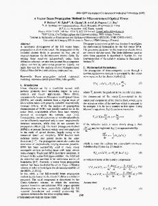
2. Incorporating Angular Deviations due to Imperfect Parallelism of Surfaces in Standard ABCD Computations We take the example of Electronically Controlled Tunable Lenses (ECTLs) [2-4]. Some tunable lens designs generally consist of an outer casing of an elastic membrane with liquid trapped inside this membranebased encapsulation. Through design or inadvertently due to manufacturing defects, the two transparent faces of a lens (i.e. the entrance and the exit apertures of a lens) can suffer from the problem of an imperfect parallelism. Such imperfect parallelism of surfaces, as shown in Fig.1, cause an extra angular ray deviation which is unaccounted for in standard ABCD models. In this paper, we introduce an extra correction angle to the angular deviation that a beam would experience from an equivalent ideal optical component. The method involves simply introducing an
additional error angle to a beam which would otherwise pass through an equivalent ideal optical component.
Fig.1 Beam angular deviation due to manufacturing defects and imperfect parallelism of surfaces
2.1. An Afocal System with one Defected or Misaligned Lens Telescopic imaging systems [5-6], beam correction systems [7] and opthalmometers [8] often deploy an afocal system which involves the use of two lenses separated by a distance which is equal to the sum of their focal lengths. Due to the widespread use of afocal systems, as an example of a slightly defected optical system, we first consider a 2-lens afocal system in which first lens (Lens 1) introduces a fixed additional angular deviation irrespective of the height or incidence angle of an incoming ray.
Fig.2 A Two-Lens System with a Defected First Lens An incoming beam is incident on the system with an initial beam height 𝑦1 and an incidence angle 𝜃1 , as shown in Fig.2. The ABCD matrix of Lens 1 with focal length 𝑓1, is given by: 𝐴 [ 𝐶
1 𝐵 = [− 1⁄ ] 𝐷 𝐿𝑒𝑛𝑠1 𝑓1
0 1]
(1)
The incident beam exits with a height ya and angle θa’ after passing through Lens 1. Here ya and θa’ of the emerging rays are calculated for a perfect lens which does not introduce any additional angular deviation due to an imperfect parallelism.
1 𝑦𝑎 ( ) = (− 1⁄ 𝜃𝑎 ′ 𝑓1
0 𝑦1 𝑦1 1) (𝜃1 ) = (− 1⁄ 𝑦 + 𝜃 ) 1 𝑓1 1 (2)
To account for an additional angular deviation 𝜃𝑒 , we add an angle 𝜃𝑒 to 𝜃𝑎 ′ to determine the actual angle of the exit ray θa. 𝑦1 𝑦1 𝑦𝑎 𝑦𝑎 0 0 ( )=( )+( )=( 1 )+( )= ( 1 ) 𝜃𝑎 𝜃𝑎 ′ 𝜃𝑒 𝜃𝑒 − ⁄𝑓 𝑦1 + 𝜃1 − ⁄𝑓 𝑦1 + 𝜃1 + 𝜃𝑒 1 1 (3) For an afocal system, i.e. two lenses of focal lengths f1 and f2 which are separated by a distance of 𝑓1 + 𝑓2, the ABCD matrix for beam propagation between the two lenses is given by: 1 𝑓1 + 𝑓2 ( ) 0 1
(4)
Beam propagation through Lens 2 with perfectly parallel interfaces is given by: 1 (− 1⁄ 𝑓2
0 1)
(5)
Therefore, after propagating through Lens 1 and Lens 2, we can find the magnitude of the lateral shift y2 and the exit angle θ2 of the beam with respect to the optical axis. 1 𝑦2 ( ) = (− 1⁄ 𝜃2 𝑓2
0 1 1) (0
𝑓1 + 𝑓2 𝑦𝑎 )( ) 1 𝜃𝑎 (6)
The overall ABCD matrix for the two-lens afocal system is given by: 1 𝑦2 ( ) = (− 1⁄ 𝜃2 𝑓2
0 1 1) (0
𝑦1 𝑓1 + 𝑓2 )( 1 ) 1 − ⁄𝑓 𝑦1 + 𝜃1 + 𝜃𝑒 1
(7) Multiplying the three individual ABCD matrices (one for each lens and one for the separation between the lenses), we obtain: 1 𝑦2 ( ) = (− 1⁄ 𝜃2 𝑓2
0 𝑦1 + (𝑓1 + 𝑓2 ) (− 1⁄𝑓 𝑦1 + 𝜃1 + 𝜃𝑒 ) 1 ) 1) ( − 1⁄𝑓 𝑦1 + 𝜃1 + 𝜃𝑒 1 (8)
1 𝑦2 ( ) = (− 1⁄ 𝜃2 𝑓2
𝑓 0 (𝜃1 + 𝜃𝑒 )𝑓1 + (𝜃1 + 𝜃𝑒 )𝑓2 − 2⁄𝑓 𝑦1 1 ) 1) ( 1 − ⁄𝑓 𝑦1 + 𝜃1 + 𝜃𝑒 1 (9)
𝑦2 ( )= 𝜃2
(𝜃1 + 𝜃𝑒 )𝑓1 + (𝜃1 + 𝜃𝑒 )𝑓2 − 𝑓2⁄𝑓 𝑦1 1
𝑓 (− 1⁄𝑓 ) ((𝜃1 + 𝜃𝑒 )𝑓1 + (𝜃1 + 𝜃𝑒 )𝑓2 − 2⁄𝑓 𝑦1 ) + (1) (− 1⁄𝑓 𝑦1 + 𝜃1 + 𝜃𝑒 ) 2 1 1 ( ) (10)
(𝜃1 + 𝜃𝑒 )𝑓1 + (𝜃1 + 𝜃𝑒 )𝑓2 − 𝑓2⁄𝑓 𝑦1 𝑦2 1 ( )=( ) 𝑓1 (𝜃 𝜃2 1 1 − ⁄𝑓 1 + 𝜃𝑒 ) − (𝜃1 + 𝜃𝑒 ) + ⁄𝑓 𝑦1 − ⁄𝑓 𝑦1 + (𝜃1 + 𝜃𝑒 ) 2 1 1 (11) A simplified form for the height and exit angle of the beam is hence given by: 𝑓 (𝜃1 + 𝜃𝑒 )𝑓1 + (𝜃1 + 𝜃𝑒 )𝑓2 − 2⁄𝑓 𝑦1 𝑦2 1 ( )=( ) 𝑓1 (𝜃 𝜃2 − ⁄𝑓 1 + 𝜃𝑒 ) 2 (12) For 𝜃1 = 0 (i.e. incoming beam is parallel to the optical axis) 𝑓 𝜃𝑒 𝑓1 + 𝜃𝑒 𝑓2 − 2⁄𝑓 𝑦1 𝑦2 1 ⇒( )=( ) 𝑓1 𝜃2 − ⁄𝑓 𝜃𝑒 2 (13) A negative value of 𝑦2 indicates beam crossing the optical axis before reaching Lens 2. It is also clear from Eq.13 that if Lens 1 does not suffer from imperfect parallelism, i.e. 𝜃𝑒 = 0, then the beam would simply exit the afocal system parallel to the optical axis, as is expected from a two lens system with no issues of imperfect parallelism.
2.2. Lateral Displacement Due to Angular Beam Steering The lens separation for an afocal system is stated in Eq.4 as: 𝑑 = 𝑓1 + 𝑓2
(14)
⟹ 𝑓2 = 𝑑 − 𝑓1
(15)
The lateral displacement or shift, 𝐷, of the beam after passing through the two-lens system is calculated as (𝑑 − 𝑓1 ) 𝑓 ⁄𝑓 𝑦1 = 𝑦1 − 𝜃𝑒 𝑑 + 𝐷 = 𝑦1 − 𝑦2 = 𝑦1 − 𝜃𝑒 𝑓1 − 𝜃𝑒 𝑓2 + 2⁄𝑓 𝑦1 = 𝑦1 − 𝜃𝑒 𝑓1 − 𝜃𝑒 (𝑑 − 𝑓1 ) + 1 1 𝑓 𝑑⁄ 𝑦 − 1⁄ 𝑦 (16) 𝑓1 1 𝑓1 1 𝐷=
𝑑𝑦1 ⁄𝑓 − 𝜃𝑒 𝑑 1
(17)
The resulting beam displacement 𝐷𝑃 at any given plane located at a distance L after Lens 2 along the optical axis is given by: 𝐷𝑃 = 𝐷 + 𝐿tan𝜃2 = ⇒ 𝐷𝑃 =
𝑑𝑦1 𝑓 ⁄𝑓 − 𝜃𝑒 𝑑 + 𝐿tan (− 1⁄𝑓 𝜃𝑒 ) 1 2
𝑑𝑦1 𝑓𝜃 ⁄𝑓 − 𝜃𝑒 𝑑 + 𝐿tan ( 1 𝑒⁄(𝑓 − 𝑑)) 1 1
(18) (19)
2.3. An Afocal System with two Defected Lenses It is evident from Eq.12 that the fixed angular deviation in the paraxial approximation simply adds to the incidence angle of the incoming beam with respect to the optical axis. If the second lens also imparts an additional angular deviation 𝜃𝑒2 , then the height and angle of the beam exiting the afocal two-lens system is given by: (𝜃1 + 𝜃𝑒 + 𝜃𝑒2 )𝑓1 + (𝜃1 + 𝜃𝑒 + 𝜃𝑒2 )𝑓2 − 𝑓2⁄𝑓 𝑦1 𝑦2 1 ( )=( ) 𝑓1 (𝜃 𝜃2 − ⁄𝑓 1 + 𝜃𝑒 + 𝜃𝑒2 ) 2 (20) For an incoming ray parallel to the optical axis i.e. 𝜃1 = 0, Eq.20 simplifies to: (𝜃𝑒 + 𝜃𝑒2 )𝑓1 + (𝜃𝑒 + 𝜃𝑒2 )𝑓2 − 𝑓2⁄𝑓 𝑦1 𝑦2 1 ( )=( ) 𝑓1 (𝜃 𝜃2 − ⁄𝑓 𝑒 + 𝜃𝑒2 ) 2 (21)
3. Conclusion We have developed a theoretical framework to compute beam propagation through lenses with parallelism defects. We modified an existing ABCD matrix for an ideal lens and incorporated non-parallel surfaces through the introduction of an angular deviation term due to non-parallel interfaces. This angular deviation adds linearly to the deviation that an ideal lens would otherwise introduce to an incoming beam. In doing so, the effects of imperfect parallelism have been accounted for in the modified beam propagation model that we propose.
References 1) H. Kogelnik and T. Li, “Laser beams and resonators,” Applied Optics, Vol. 5, No.10 pp.1550-1567, 1966. 2) Optotune Switzerland AG, “Fast Electrically Tunable Lens EL-10-30 Series,” (2016). 3) Parrot SA Confidential, “Arctic 316 Arctic 316-AR850,” 2016. 4) B. H. W. Hendriks, S. Kuiper, C. A. Renders, and T. W. Tukker, “Electrowetting-based variable-focus lens for miniature systems,” Optical review, Vol.12, No.3, pp.255-259, 2005. 5) M. H. Spencer, and L. G. Cook, “Three field of view refractive afocal telescope,” U.S. Patent 5,229,880, issued July 20, 1993. 6) R. B. Johnson, “Very broad spectrum afocal telescope,” In International Optical Design Conference, International Society for Optics and Photonics, pp. 711-717, 1998. 7) C. Y. Han, Y. Ishii, and K. Murata, “Reshaping collimated laser beams with Gaussian profile to uniform profiles,” Applied optics, Vol.22, No.22, pp.3644-3647, 1983. 8) M. G. P. Frederic, “Opthalmometer having afocal lens system,” U.S. Patent 3,290,927, issued December 13, 1966.