Calibrating a large-scale traffic flow simulator Laura Bieker, Julia Ringel, and Peter Wagner
∗
Institute of Transport Systems, German Aerospace Centre (DLR), Berlin, Germany
ABSTRACT
the full paper, here concentration is on the urban scenario. It is located in Berlin, Germany, Ernst-RuskaThis contribution demonstrates how to perform cal- Ufer, see the Figure 1 for the layout. This four-lane ibration and validation for the open source traffic flow micro-simulation SUMO [1]. Preliminary results for a real-world scenario are presented. This serves as an example how a black box model can be calibrated and validated without knowing and accessing the inner workings of the simulation model. Here, ”black box” is from the view-point of an traffic analyst, which is a valid view for many researchers despite SUMO being an open source program. Keywords: Calibration, validation, traffic flow simulation, real-world scenarios
INTRODUCTION One motivation behind the current research interest in microscopic traffic flow models was the idea, that they should describe reality to such a level of detail, that in fact no real calibration of the model parameters needs to be carried out – they could be measured directly, and then put directly into the model description, leaving to the analyst only validation to perform. For reasons not very well-known so far, this has not worked, therefore there is still the need to perform the calibration and validation part before a micro-simulation (or any other traffic simulation model) could be used to describe real-world behaviour [2]. This task has sparked a large outbreak in scientific interest in this matter, manifesting in a large number of publications dealing with different aspects of calibration and validation, see [3, 4, 5, 6, 7, 8, 9, 10, 11, 12, 13] for an incomplete list of references.
TECHNICAL DESCRIPTION STUDY AREAS
AND
Two different study areas are currently regarded: a small inner-urban scenario where a large amount of data is available, and secondly, a couple of freeway scenarios which have good data coverage, but not as well as in the urban scenario. The latter will be discussed in ∗ Institute of Transport Systems, DLR, Rutherfordstraße 2, Berlin, Germany, Tel: +49 30 67055-237, Fax: +49 30 67055291, E-mail:
[email protected]
Fig. 1: Logic layout of the study area. Only the structures used in this study are shown.
road (two lanes per direction) is equipped with around 40 loop detectors, in addition to other data like traveltimes from a fleet of taxis, weather data which are so far not used, because the actual precision of the microsimulation do not allow to tell apart whether the difference between simulation and reality is due to weather conditions, errors in the data or errors in the simulation itself. One day has been used, where there was considerable spill-back from the downstream bottleneck, in this case the 11 January 2011. To run the SUMO simulation [14, 1, 15], it needs as input routes through the network. Each vehicle that enters the study area in the simulation is equipped with such a route that had to be computed by a number of preprocessing steps that depend on the scenario at hand. In this case, since the network is fairly simple, the routes are easy to generate, Figure 1 demonstrates that the study area is surrounded by loop detectors. Although the data given do not allow for a complete specification of the routes of the vehicles, it can be expected that the error that is generated by the route construction process is not very large. Within this work, only the eastbound traffic is regarded so far. Traffic enters at loop detector MQ 11, and it leaves at loop detector MQ 42. The main detectors for testing the quality of the simulation are the detectors MQ 31 and MQ 22, they are labelled in Figure 1, too. This is due to the fact, that it is the most difficult to model, since further downstream (especially for the late afternoon rush-hour) a strong bottleneck causes a spill-back into the study area, whose spatiotemporal extension should be modelled by the simula-
2nd International Conference on Models and Technologies for Intelligent Transportation Systems 22-24 June, 2011, Leuven, Belgium
tion. However, there is a mechanism needed that serves to transport this spill-back into the study area, and this is provided by the speed measurements of the secondlast down-stream detector. (The last one is ignored so far, because it is downstream of a traffic-actuated traffic signal, for which the detailed switching sequence is not known.) The general recipe for doing this coupling (which is valid for any microscopic simulation) is that
from the measured data in MQ 42 – in contrast to real VSS, it can change the speed limit within one time-step of the simulation. However, a certain abstraction has been chosen as the control speed of the VSS, as shown in Figure 2.
RESULTS
The results obtained so far are displayed in Figure 3. • either the speed can be used to couple the spillIt could be seen, that on this level of description, the back into the study area [16], • or the number of vehicles by using a so called virtual traffic light [5] – it switches to red, if more vehicles than actually observed have left the study area, and goes back to green, if this number is smaller, • or the settings of a real traffic light at the outlet of a study area could be used.
120
Since the virtual traffic light creates strong, possibly artificial fluctuations, and the detailed parameters of the actual traffic light directly downstream of detector # 41 was not available within this study, this work used the approach of controlling the speed of the vehicles leaving the study area. Within SUMO, several
●
80
100
Velocity used for VSS in Simulation
● ●
● ●● ●
●
60
●
●● ● ● ●● ● ● ● ● ● ● ● ● ● ● ● ● ● ● ● ● ●● ● ● ●● ● ●●● ● ● ● ● ● ● ● ● ● ● ●● ●● ● ● ●● ● ● ●● ●● ● ● ● ● ● ● ● ● ● ●●●● ●●● ● ●● ● ● ●● ● ● ● ●● ● ● ● ● ● ● ● ● ● ● ● ● ● ● ● ●● ● ●●●● ● ● ● ● ● ● ● ●● ● ● ●● ●● ● ●● ●● ● ● ●● ● ● ● ● ● ● ● ●● ●● ● ● ●●● ● ● ●● ●● ● ●● ● ●● ● ●● ● ● ● ●● ● ●●● ● ● ● ● ●●●●● ● ●● ● ● ●● ● ● ● ●● ● ● ●●● ● ●● ●● ● ● ● ●● ●● ●● ● ● ● ●● ● ●● ● ●● ● ●● ● ● ● ●● ● ● ●● ● ● ● ● ● ●● ● ●● ● ●●●● ●● ● ● ● ●● ● ● ●● ● ●● ●● ● ● ●● ● ● ●● ● ● ● ● ● ●● ●●●●● ● ● ●●● ● ● ● ●● ●● ● ● ●● ●●● ● ● ● ● ●● ● ●●●● ● ● ● ●●● ● ● ●● ● ● ●● ●● ● ●● ● ●● ●● ● ● ● ●● ● ● ● ● ● ● ●● ● ●● ●●● ● ●● ● ●● ● ●● ●● ● ● ● ● ●● ●●●● ● ● ●● ● ●●● ● ●● ● ● ● ● ●● ●● ● ●● ●● ● ● ● ● ●●● ● ●● ●● ● ●● ● ● ● ●● ●●● ● ●●●● ● ●●● ● ●● ● ● ●● ● ● ● ●●● ●● ●●● ● ● ●● ● ● ● ● ●●●● ● ● ● ● ● ●● ●●● ●● ● ● ●●●● ● ● ●● ● ●● ●● ● ● ●●●● ● ●● ● ●● ●● ●● ●●● ● ●●● ● ● ● ● ● ●● ● ●●● ● ●●●●● ●●● ● ● ● ● ●● ● ●● ● ●●● ●● ● ●● ● ●●● ●● ●●● ●● ● ● ●●● ● ● ● ● ● ● ●● ●●●●●● ●● ●● ●●● ● ● ● ●● ● ● ● ●●● ●● ● ●●● ● ●● ●● ●● ● ● ●● ● ●● ●●● ●●● ●●●● ●●● ● ● ●●● ● ●● ●● ● ● ●● ●● ●●●●●●●●● ● ● ● ●● ● ● ● ● ● ● ● ● ● ● ●● ● ● ● ●●● ● ●●● ●● ● ●● ● ●● ●● ● ● ● ●● ●●●● ● ●●●●●● ● ●● ●● ● ●● ●● ● ● ●●● ● ●● ● ●●● ●●● ●● ●● ● ● ● ● ●●●●●● ● ● ● ● ●●● ●●● ● ● ●●● ● ●● ●● ●● ●●● ● ● ●● ● ● ●● ● ●●●● ●● ● ●●● ●● ● ● ●● ● ●●● ● ●● ●● ●●●●● ●● ●● ● ● ● ●● ● ● ●●●●● ●●●●● ●●●● ●●● ●●● ●●● ●● ●●● ● ● ●● ●● ● ● ●● ●● ● ●● ●●●● ● ● ● ● ● ●● ● ●●●● ●●● ● ● ●● ● ●● ●●● ● ● ●● ● ●● ● ● ● ● ● ● ● ●● ●●● ●● ●● ● ●● ●● ● ● ● ●● ● ● ● ● ●● ● ● ●●● ●● ●●● ● ● ●● ● ●●● ● ●● ● ● ●● ● ●●●● ● ●● ●● ●●● ● ● ●● ●● ● ● ●●● ● ● ●● ● ●● ● ●● ● ●● ●● ●● ● ● ● ● ● ●● ●● ● ● ●● ● ●● ●● ● ●● ● ● ●● ●●●●●●● ●●● ● ●●●● ● ● ●● ● ● ● ● ● ● ● ●●●●● ●● ●● ● ●● ●●● ●● ●● ● ● ●●● ● ● ● ● ● ● ● ●●● ● ●● ● ● ● ● ● ● ●●●● ●●● ● ● ●● ● ● ●● ●● ● ●● ● ●● ● ●●● ●● ●● ●● ●● ● ●●● ● ● ●● ●●● ● ● ●● ● ●● ● ● ● ● ●● ● ●● ●● ●● ● ● ● ● ● ● ● ●● ● ● ●●● ● ● ●●● ● ●● ● ●●● ● ●●●●● ●● ● ● ●●●●● ●●●●●● ● ● ●● ●●● ● ●● ● ● ●● ●●●● ● ●● ●● ●● ●● ● ●● ●●● ● ●● ●● ●● ● ●●●●● ● ● ● ●●● ● ● ●● ● ●● ● ● ● ● ●● ●●● ● ● ● ●● ●●● ●● ●●● ● ● ●●● ● ●●● ●●● ●●●● ●● ● ●● ●● ● ●● ● ●● ● ● ● ●●●●●● ● ● ● ● ●● ● ● ●● ● ●●●● ● ● ● ●●● ● ●● ● ● ● ●●● ● ● ● ●●●●●●● ●● ●● ●● ● ●●● ● ● ● ● ●● ●● ● ● ● ●● ● ● ● ● ● ●● ●● ● ● ● ● ● ● ●● ● ● ●●●● ● ● ● ● ● ● ● ● ●●● ●● ● ●● ● ●● ●●● ● ● ●● ● ●● ● ●● ●●● ●●●● ●● ● ● ● ● ●● ● ●● ● ● ●● ●●● ● ● ● ● ● ●●● ●● ●● ● ● ●● ●●● ● ●● ● ●● ● ●● ●● ● ● ●●●● ● ● ● ● ●● ●● ● ● ●● ●● ● ● ●● ● ● ●● ● ●● ●●●●● ● ●● ● ●●●● ● ●● ● ● ● ● ● ●● ● ● ● ● ●●● ● ● ● ● ● ● ● ● ●●●● ●● ● ●●●●● ●● ● ●● ●● ●●● ● ● ● ● ●●● ● ● ●● ● ●●● ● ●● ●● ● ● ● ● ● ● ● ●● ●●● ● ●● ● ●●● ● ●● ● ● ●● ● ●●● ● ● ● ●● ● ● ● ● ● ● ● ●● ● ● ● ● ● ● ● ●● ● ●● ● ●●●● ●●● ●● ● ●●● ● ● ●● ● ● ● ●● ● ●● ● ● ● ●● ● ● ● ●● ● ●● ●● ● ● ●●● ●●●●● ●● ● ● ●●● ● ● ● ● ● ● ●● ● ● ●● ● ● ● ●● ● ●●● ● ●●●● ● ●● ●● ● ● ● ● ● ● ● ●● ● ● ● ● ● ● ●● ● ● ● ●● ●●● ●●●● ●●●● ● ● ● ● ●● ● ●● ● ● ●●● ● ● ● ● ● ●●● ● ●● ● ● ● ●● ● ● ● ● ● ● ● ● ● ●● ● ● ● ●● ● ● ● ● ●● ● ● ● ●● ● ●● ● ● ● ● ●● ●● ● ●● ● ● ●●● ● ● ●● ● ● ●● ● ● ● ● ●● ● ● ● ● ●● ●●● ● ●● ● ●● ● ● ●● ● ● ●●● ● ● ●● ● ● ●● ● ● ● ● ● ●●●● ● ● ● ● ●●● ●●●● ● ● ● ● ●● ●●● ● ●● ●●● ●● ● ●● ● ● ●● ● ●● ● ● ●● ● ● ●●●●● ● ● ● ●● ●●●● ● ●● ●● ● ●● ● ● ●● ● ●● ●● ●●● ● ● ●● ●● ● ●● ●●● ● ● ● ● ●● ● ●● ● ●●● ● ● ● ●●●● ● ● ●● ●● ●● ● ● ● ●● ●● ● ● ●●●● ●●●● ●● ●● ●●●● ● ● ● ● ● ●● ● ● ● ●● ● ● ● ●● ● ● ●● ●● ●● ●●● ● ●● ● ● ●● ●● ● ●● ● ●● ●● ● ● ● ●● ●●● ●●●● ● ●●●● ● ● ●● ●●● ● ● ● ● ● ● ● ● ● ● ●● ●● ● ●● ●● ●●●●● ● ● ●● ●● ● ●● ●● ● ●● ● ●●●● ● ● ●● ● ●● ●●● ● ●●● ●● ● ● ●● ● ●●● ● ●● ●●●● ●● ●● ● ● ● ● ●● ● ● ●● ● ● ●
0
20
40
Velocity in [km/h]
Velocity Messured at #42, behind the Traffic Light
0
20000
40000
60000
80000
Time in [s]
Fig. 2: Speed data at loop detector MQ 42, and the resulting VSS function.
approaches can be used to perform this task. Possibly the simplest one is by using SUMO’s VSS (variable Fig. 3: Speed as function of time for the real data as well as for the simulation, for the first (MQ 31) and the speed sign) class. The study area is extended by ansecond upstream (MQ 22) detector. other short link (between MQ 41 and MQ 42, by ignoring the intersection completely) which is controlled by such a VSS, and the VSS yields its speed limits directly simulation reproduces reality not too bad. The calibra-
2nd International Conference on Models and Technologies for Intelligent Transportation Systems 22-24 June, 2011, Leuven, Belgium
tion has been done so far manually, without a dedicated interesting questions related to the benefit of such an non-linear optimization of the distance between reality endeavour. and simulation. Most noteworthy is the fact, that the spill-back in the example reaches detector # 31, but REFERENCES not the detector # 22 (although a small effect could be seen at this detector, both in the simulation as well as [1] SUMO – Simulation of Urban MObility see in the real data), and this is reproduced faithfully by http://sumo.sf.net last access: 13. Feb. 2011. the simulation. [2] Law, A. M. and Kelton, W. D. (2000) SimulaQuantitatively, the results are not that convincing so tion Modelling and Analysis, McGraw-Hill, 3rd far. While the average and median errors in the flows edition. and in the speeds for both detectors are well below 1 veh/min and 1 km/h (for the speeds), respectively, the root-mean-square errors are about 3 veh/min and [3] Antoniou, C., Ben-Akiva, M., and Koutsopoulos, H. N. (2007) IEEE Transactions on Intelligent about 5 km/h (inter-quartile distance q75 − q25 for the Transportation Systems 8, 661–670. upstream detector MQ 22) and 10 km/h, roughly a 20 % error for the downstream detector MQ 31. The [4] Barcelo, J. and Casas, J. (2004) In Proceedings of detailed numbers are summarized in Table 1. the 83th Transportation Research Board Annual Meeting : . Table 1: Performance indices of the simulation. Speed error values are in km/h, while flow error values are in veh/min. For the speeds, the average speed is around 50 km/h.
error mean r.m.s. median q75 − q25
flow (MQ22) -0.6 3.73 0 3.0
speed (MQ22) 0.18 18.18 0 5.28
flow (MQ31) -0.58 3.29 0 3.0
speed (MQ31) 0.84 21.31 0.42 10.11
CONCLUSIONS The results demonstrated so far show, that even without an explicit calibration, a microscopic traffic flow simulation describes reality not too wrong. This may have several reasons: the obvious one is that the simulator is well designed and describes reality quite well. However, it could well be the fact, that the reality that has been used limits and determines strongly the outcome of such a simulation. In other words: even a bad model has no chance to produce a bad fit. What rules against this possibility is especially the fact that a highly non-trivial scenario has been used to test the simulator. Clearly, much more detailed and many more studies like the one described here are needed to better understand the interplay between simulation and reality. Nevertheless, these results could be improved further by trying to estimate a best set of SUMO parameters by an automatic minimization of, for example, the difference between the simulated speed curve vˆ(t) and the measured one v(t). This will be done for the presentation at the conference, and it might lead to additional
[5] Brockfeld, E., K¨ uhne, R. D., Skabardonis, A., and Wagner, P. (2003) Transportation Research Records 1852, 124 – 129. [6] Ciuffo, B. and Punzo, V. (2010) In Proceedings of the 89th Transportation Research Board Annual Meeting : . [7] Cremer, M. and Papageorgiou, M. (1981) Automatica 17, 837–843. [8] Dowling, R., Skabardonis, A., Halkias, J., McHale, G., and Zammit, G. (2004) Transportation Research Records 1876, 1–9. [9] Hollander, Y. and Liu, R. (2008) Transportation: Planning, Policy, Research, Practice 35, 347–362. [10] Ossen, S. and Hoogendoorn, S. P. (2008) Transportation Research Records 2088, 117–125. [11] Thiemann, C., Treiber, M., and Kesting, A. (2008) Transportation Research Records 2088, 90–101. [12] Punzo, V. and Ciuffo, B. (2009) Transportation Research Records 2124, 249–256. [13] Toledo, T., Koutsopoulos, H. N., Davol, A., BenAkiva, M., Burghout, W., Andrasson, I., Johansson, T., and Lundin, C. (2003) Transportation Research Records 1831, 66–75. [14] Krajzewicz, D., Hertkorn, G., R¨ossel, C., and Wagner, P. (2002) In A. Al-Akaidi, (ed.), Proceedings of the 4th Middle East Symposium on Simulation and Modelling (MESM 2002), : SCS European Publishing House. [15] Brockfeld, E., K¨ uhne, R. D., and Wagner, P. (2004) Transportation Research Records 1876, 62 – 70.
2nd International Conference on Models and Technologies for Intelligent Transportation Systems 22-24 June, 2011, Leuven, Belgium
[16] Brockfeld, E., K¨ uhne, R. D., and Wagner, P. (2005) Transportation Research Records 1934, 179 – 187.