003_Bischetti(569)_23
1-12-2010
9:48
Pagina 23
J. of Ag. Eng. - Riv. di Ing. Agr. (2010), 3, 23-35
CALIBRATION OF DISTRIBUTED SHALLOW LANDSLIDE MODELS IN FORESTED LANDSCAPES
Gian Battista Bischetti, Enrico Antonio Chiaradia
1. Introduction In mountainous-forested, soil mantled landscapes all around the world, rainfall-induced shallow landslides are one of the most common hydro-geomorphic hazards [Sidle 1985]. Such hazards frequently impact the environment and human lives and properties. In order to manage and protect human interests, landslide susceptibility maps must be produced [Guzzetti 1999] and several models have been proposed in the last decade [Montgomery 1998; Borga 2002; Casadei 2003; Claessens 2007; Talebi 2008; Kuriakose 2009]. The most common approach to shallow landslide modelling combines, in a GIS framework, simplified steady state topography-based hydrological models with the infinite slope scheme [Dietrich 1993; Montgomery 1994; Wu 1995; Pack 1998; Dietrich 1998; Borga 2002; van Beek 2002; Simoni 2008]. The success of such an approach is due to the simplicity of the steady-state hydrologic approach and the power of GIS technology in managing elevation and spatially distributed data. Although several issues affect the modelling results, the approach has been proven to be very useful and many Authors adopted it [e.g. Dietrich 1998; Wu 1995; Borga 2002; Montgomery 1994; Duan 2000; Pack 1998, 2005]. Among the open issues that still affect such an approach, the main ones are: i) the effect of the algorithm adopted to identify flow directions and contributing area [Huang 2007; Santini 2009], ii) the effect of DEM resolution and accuracy [Claessens 2005], iii) the effect of a steady state or dynamic approach to water pore pressure within the soil [Borga 2002; Rosso 2006], iv) the role of vegetation in soil resistance estimation [Kuriakose 2009], v) the evaluation of the model’s performance [Huang 2007]. In the present paper we focus on the last two
___________ Paper received 04.12.2009; accepted 25.05.2010 G.B. BISCHETTI, Professore Associato, E.A. CHIARADIA, Assegnista di Ricerca, Dipartimento di Ingegneria Agraria – Università degli Studi di Milano, Via Celoria 2 – 20133 Milano,
[email protected]
points, applying a spatially distributed model for slope stability estimation, the “Stability INdex MAPping - SINMAP” [Pack 1998, 2005], to a small forested pre-Alpine catchment, adopting different calibration approaches. 2. Material and methods 2.1 The assessment of shallow slope stability model results According to Borga [2002] two types of errors can be identified in modelling slope instabilities: (1) a site is identified by the model as unstable, but no evidence of instability can be observed, (2) a site is predicted as stable, but instabilities have been observed. The first type of error indicates that the model tends to over-predict areas potentially subject to shallow landsliding, whereas the second indicates that the model does not adequately describe the processes that caused the instability process. In principle the first type of error could not be a true error because the predicted unstable condition should be viewed as an indication of a proneness to instability; it has not still occurred but it can manifest in the future, especially in very steep areas. The second type of error could have serious consequences when the considered model is applied to hazard mapping and it must be minimized. To evaluate the performance of stability models, it is common to use the so-called Success Rate (SR) [Montgomery 1994; Borga 2002; Duan 2000]. It is the ratio between the number of observed landslides actually occurred in predicted unstable areas (NUR) over the total number of observed landslides (NUO): (1) SR=NUR/NUO SR does not consider stable areas, where prediction can be correct or not. Generally, it has been recognized that adopting SR as a performance indicator, slope failure is over-predicted [Borga 2002; Casadei 2003; Huang and Kao]; as an extreme case, for example, if the whole area is classified as unstable, the resulting SR will be 100%.
003_Bischetti(569)_23
1-12-2010
9:48
Pagina 24
24 Huang [2006] and Rosso [2006], recently proposed more complex indexes. Huang [2006] considered also the successfully predicted stable areas developing a Modified Success Rate, which is an average between the success in predicting unstable and stable areas: (2) where SR are the successfully predicted stable cells and SO are the total number of actual stable cells. Rosso [2006] considered a combinations of four sub-indexes: Iav=average(UR/UO, UR/Uc, SR/SO, SR/SC) (3) where: UO is the number of observed unstable cells, UC is the number of simulated unstable cells, UR is the number of rightly simulated unstable cells, SC is the number of simulated stable cells. UR/UO is an indicator of the model efficiency to identify landslides, UR/Uc can be viewed as an indicator of the manifested instability over the potential instability, SR/SO is an indicator of the model efficiency to identify stable areas, SR/SC is the reciprocal of UR/Uc. In the case of small instabilities, which have an extension of the order of one or a few hundreds of square meters [Dietrich 2007; Deb 2009], it can be assumed that each observed landside occupies one cell in a 10 m or 15 m grid size. The number of observed landslides that actually occurred in predicted unstable areas, then, can be approximated to the rightly simulated unstable cells and the total number of observed landslides can be approximated to the observed unstable cells: and
NUR= UR
Huang [2006], then, represents the best way to evaluate stability model performance. Due to the fact that it is more difficult to predict actual unstable areas (see the first type of errors as reported at the top [Carrara 1995; Borga, 2002]) we think that the two indexes should not have the same weight, as in the case of MSR, but SR should prevail. Based on such consideration, we introduce a weighted average index (WMSR) that gives an arbitrarily weight of 2/3 to SR and a weight of 1/3 to SR/SO. 2.2 SINMAP Among the different models that have been proposed in the last years in the field of rainfall-triggered shallow landslides, the most widely applied are SHALSTAB [Dietrich 1998] and SINMAP (Stability INdex MAPping) [Pack 1998], which are freely distributed. Such models couple the infinite slope stability model and the assumption of hydrologic steady state to compute pore water pressure in the soil. In the present work, the SINMAP model was preferred to SHALSTAB due to its capability to manage slope stability from a probabilistic perspective [Meisina 2007]. SINMAP has also been tested in different landscapes and conditions [Morrissey 2001; Zaitchik 2003; Calcaterra 2004; Lan 2004; Meisina 2007]. The original version of the model is distributed under a GNU General Public Licence version as an extension of a commercial GIS software; in the present work we used a version re-built for the open-source software MapWindow [Chiaradia 2009]. In the infinite slope stability approach, the Factor of Safety (FS) is [Hammond 1992]:
NUO= UO (5)
SR=UR/UO The index proposed by Huang [2006] (MSR), as a consequence, results in the average between the first and the third of the sub-indexes of Rosso [2006]: MSR=0.5(UR/UO + SR/SO)
(4)
Recalling the two types of errors that may occur in slope stability modelling: – high values of SR (and UR/UO) indicate that the model may fail, falling in the first type of error (sites are identified by the model as unstable, but no evidence of instability can be observed) and low values that the model may fail falling in the second type of error (sites are predicted as stable, but instabilities have been observed); – UR/Uc and SR/SC do not give any real indication concerning the model performance; – high values of SR/SO indicates that the model is prone to fail, falling in the second type of error and low values that the model is prone to fail, falling in the first type of error. The combination of SR and SR/SO as proposed by
where (fig. 1) cs is the soil cohesion (kPa), cr is the additional root cohesion (kPa), γs is the soil unit weight (kN/m3), γw is the water unit weight (kN/m3), D is the vertical soil depth (m), Dw is the vertical water depth (m), β is slope angle (°) and φ is the internal friction angle (°) Introducing the variables:
(6) where h=D cosβ is soil thickness equation (5) can be rewritten and FS can be expressed as: (7) Adopting a modified version of the TOPMODEL approach [Beven 1979] the relative wetness (w) can be evaluated as: (8)
003_Bischetti(569)_23
1-12-2010
9:48
Pagina 25
25
Fig. 1 - infinite slope stability scheme (after Hammond [2009])
where T is the transmissivity (m2/h), R is the steady state recharge that is an estimation of the lateral discharge (m/h), a is the upslope drained area per unit contour length (m2/m). C, R/T and φ are the calibration parameters of SINMAP and they are introduced as minimum and maximum values, considered uniformly distributed. According to the combination of the parameters, the values FSmin and FSmax can be obtained; on such a basis, to define the level of stability of the terrain, SINMAP introduces a Stability Index (SI) (fig. 2). Where FSmin>1 the terrain is considered stable and SI= FSmin, where FSmin1)), where FSmax1)=0, the terrain is considered unconditionally unstable. Arbitrarily, SINMAP considers stable the terrain where SI>1.5, moderately stable where 1.5