Call-Routing Schemes for Call-Center Outsourcing - Semantic Scholar

Call-Routing Schemes for Call-Center Outsourcing

Noah Gans

Yong-Pin Zhou

OPIM Department The Wharton School University of Pennsylvania Philadelphia, PA 19104

Dept. of Management Science School of Business Administration University of Washington Seattle, WA 98195

∗

Draft of October 19, 2005

Companies may choose to outsource parts, but not all, of their call-center operations. In some cases, they classify customers as high or low-value, serving the former with their “in house” operations and routing the latter to an outsourcer. Typically, they impose service-level constraints on the time each type of customer waits on hold. This paper considers four schemes for routing low-value calls between the client company and the outsourcer. These schemes vary in the complexity of their routing algorithms, as well as the sophistication of the telephone and information technology infrastructure they require of the two operations. For three of these schemes, we provide a direct characterization of system performance. For the fourth, most complex, scheme we provide performance bounds for the important special case in which the service requirements of high and low-value callers are the same. These results allow us to systematically compare the performance of the various routing schemes. Our results suggest that, for clients with large outsourcing requirements, the simpler schemes that require little client-outsourcer coordination can perform very well.

∗

Research supported by the Wharton Financial Institutions Center, The Fishman-Davidson Center for Service and

Operations Management, the Center for International Business Education and Research at University of Washington, and NSF Grant SBR-9733739.

1

Introduction

Many companies choose to outsource parts of their call-center operations. That is, rather than serving their own customers, they subcontract part or all of their capacity to a company that specializes in call-center operations. Recently, this type of outsourcing has grown to become a global industry. For example, Convergys Corporation, a US-based outsourcer with worldwide operations, reported 2003 revenues of $1.5 billion for its Customer Management Group, a division with 25,000 customer service representatives (CSRs) [16, 17]. Wipro Spectramind, a large India-based outsourcer, reports that it has 9,300 employees who handle more than 4 million calls and 500,000 emails each month [50]. A common reason for outsourcing is to lower costs. Human resources expenses associated with CSRs typically account for 60–70% of call-center operating expenses. Outsourcers often have lower wage structures, which allow them to operate with a lower cost per call. For example, Wipro Spectramind reports that it typically provides 75% savings in labor costs to its clients [49]. At the same time, companies that use outsourcers may continue to serve a significant fraction of their incoming calls. In one scheme, they classify their customers as belonging to one of two types: high-value customers, who are currently or potentially profitable; and low-value customers, who will never be highly profitable. The high-value customers are considered to be an important corporate asset, and they are served by “in house” operations that the service provider trains and manages itself. The low-value customers are considered to be a “nuisance” and are routed to an outsourcer that provides a lower cost to serve but has less highly trained CSRs. Modern telephone infrastructure enables the identification of arriving calls as coming from high or low-value customers, as well as the subsequent routing of calls. Typically, client companies impose service-level constraints on the time each type of call spends waiting on hold. Common constraint forms include upper bounds on the average speed of answer (ASA), the average time calls spend waiting on hold, as well as upper bounds on fractiles of the waiting-time distribution. An example of the latter is “80% of the calls must be handled in 20 seconds or less.” These types of constraints are applied to both low-value and high-value customers, although the specific level of service may differ. Together with projections concerning the arrival rates and service times of incoming calls, these service-level constraints drive lower bounds on the numbers of CSRs that must work during a given period. Given adequate capacity to serve high-value customers, the service provider’s pool of CSRs will generally have additional capacity available to handle some low-value calls as well. This may be due to shift scheduling constraints, which force some planning periods to have a higher-than-necessary staffing levels. (See §3.2 in Gans et al. [20].) Even when the number of in-house CSRs is the absolute minimum required to meet the high-value customers’ service-level constraint, they may still have some capacity to take the low-value calls opportunistically, rather than on-demand. Service providers have economic incentives to make use of this excess capacity. Outsourcing

1

Type-H calls

Type-L calls accept

In-House CSRs

Type-H calls

reject

accept

Outsourcer CSRs

In-House CSRs

a) Dedicated In-House CSRs, Overflow

Type-H calls

In-House CSRs

Type-L calls reject

Outsourcer’s CSR’s

b) Pooled In-House CSRs, Overflow

Type-L calls

Type-H calls

In-House CSR’s

Outsourcer CSRs

c) Dedicated In-House CSRs, “Inverted V” Network

Type-L calls

Outsourcer’s CSR’s

d) Full Pooling Using an “N” Network

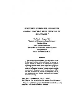
Figure 1: Routing Schemes for Type-L Calls contracts commonly include volume-based (per-call) or capacity-based (per-agent-per-hour) fees. (For example, see [28, 29].) By taking some low-value calls in-house, the service provider can reduce some of these variable outsourcing costs. In addition, a company may consider its in-house CSRs to be of higher quality than its outsourcer’s – with better training, a more neutral accent, etc. – and prefer to use in-house CSRs as a first choice, when they are available. The use of an outsourcer to handle some, but not all, low-value customers requires coordination between the two companies, both in the staffing of agents and in the routing of calls. Figure 1 depicts four schemes that vary in both the degree of coordination and resulting system complexity. In all of the figure’s panels, type-H calls come from high-value customers and type-L calls from low-value ones. Panel (a) displays the simplest scheme. Here, type-H calls are served by a dedicated group of inhouse CSRs, and any excess in-house capacity is dedicated to serving low-value calls. An “overflow” scheme is used for routing low-value calls: if an arriving type-L call finds a type-L, in-house CSR

2

idle, then the call is taken in house; otherwise it overflows to the outsourcer, where it queues and is served first-come-first-served (FCFS). We call this an overflow scheme with dedicated agents, or a dedicated-overflow scheme. Note that, because capacity for high and low-value customers is not pooled under this dedicated scheme, there will be instances at which both type-H calls are queued and in-house CSRs, dedicated to type-L calls, are idle; and vice versa. At these moments, a more complex routing scheme might be able to take fuller advantage of idle in-house capacity, thereby reducing outsourcing costs. Panel (b) depicts a scheme which more fully uses idle in-house CSRs by pooling high and lowvalue customer calls, but it does not pool capacity between the client company and the outsourcer (i.e. it uses an overflow scheme). We call this a pooled-overflow system. Routing decisions in the pooled-overflow system can be much more complex than in the dedicated scheme. In particular, the decision to process an arriving type-L call in house now depends on the state of all in-house CSRs, rather than just the availability of (at least) one of the in-house CSRs that is dedicated to type-L calls. At the same time, under both of the overflow schemes there will still be instances at which there exist idle in-house CSRs and type-L calls queued at the outsourcer. Panel (c) displays an alternative scheme in which in-house CSRs dedicated to handling type-L calls are pooled with the outsourcer’s agents, and they can all access a common type-L queue. In this system, the routing options for type-L calls take the form of an “inverted V” network. (See Garnett and Mandelbaum[22], Gans et al. [20].) Accordingly, we call this scheme inverted-V. To minimize the number of type-L calls handled by the outsourcer, the client company can specify that type-L calls are preferentially routed to its CSRs whenever one of the agents it has dedicated to type-L calls is available. Panel (d) depicts a routing scheme that pools across all in-house CSRs, as well as between the client company and the outsourcer. As in the inverted-V scheme, type-L calls are held in a common queue, and as in the pooled-overflow scheme all in-house CSRs may take both type-H and type-L calls. Given the form of the routing options, this scheme is commonly called an N-network scheme. (See Garnett and Mandelbaum[22], Gans et al. [20]). We note that the four schemes represent choices concerning the pooling of capacity across each of two dimensions. The left two panels’ schemes partition in-house capacity between type-H and type-L calls, while the right two panels’ systems pool in-house capacity across both types of calls. Similarly, the top two panels show schemes in which type-L calls overflow from the in-house group of CSRs to the outsourcer, while the bottom two panels depict schemes in which a common queue allows the pooling of type-L capacity across the two organizations. Thus, the N-network shown in panel (d) has the most ability to pool, but this benefit comes at the cost of more difficult routing controls and more stringent requirements for telecommunications infrastructure. In the overflow schemes, information concerning the occupancy of in-house CSRs is available from the client company’s local automatic call distributor (ACD), and routing decisions are executed by 3

the client company’s private automatic branch exchange (PBX). Thus, the decision of whether to serve an arriving type-L call in house or to have it overflow can be made and executed locally at the client, without having to coordinate with the outsourcer. The inverted-V network requires that type-L calls be held in a common queue and routed directly either to the client’s or outsourcer’s CSRs. This can be accomplished by having the client’s and outsourcer’s common long-distance carrier, the so-called public service telephone network (PSTN), hold all type-L calls in queue. (In voice over internet protocol (VOIP) systems, the role of the PSTN can be played by a so-called “hosted service” provider. See Dawson [18].) Whenever a type-L call arrives, the PSTN polls, first the client then the outsourcer, to see if an agent is available. Similarly, whenever an agent becomes available at either the client or the outsourcer, that call-center’s ACD polls the PSTN to deliver a call, if there exists any in queue. While the inverted-V scheme requires that calls be queued at the PSTN, it does not require complex coordination among the client, the outsourcer, and the long-distance carrier. Furthermore, the extra costs of holding calls at the PSTN may be offset by reductions in line charges associated with the overflow schemes. Specifically, each time a call overflows from the client to the outsourcer, an extra telecommunications link is established. That link may be owned by the PSTN, in which case a charge is incurred per call, or it may be privately owned by the client and outsourcer. Finally, full operation of the N-network requires that detailed occupancy information be collected from the client’s and outsourcer’s ACDs and fed back to a PSTN, which then uses the agent and queue occupancies at both locations to make complex routing decisions. Occupancy updates and routing decision must be made in real time, each time a call arrives or a CSR becomes free. Thus, while the N-network shares the line-charge advantage of the inverted-V scheme, the telecommunications and information technology infrastructure required to support its remote coordination is significantly more sophisticated. In this paper, we investigate the relative effectiveness of these schemes, analyzing Markovian versions of the systems. The arrival processes of type-H and type-L calls are stationary and Poisson, with respective rates of λH and λL . Service times of type-H calls are independent and identically distributed (i.i.d.), exponentially-distributed random variables with mean 1/µH , and type-L service times have i.i.d., exponential distribution with mean 1/µL . The arrival processes and service times are assumed to be independent of each other, as well as of the system state. Our main focus is the important special case in which service-time distributions and service-level standards are uniform across calls. When the contents of high and low-value customers’ calls are roughly the same, we can directly characterize effective routing and staffing policies for the invertedV and both overflow systems. When, in addition, service-level standards are the same across types, we can construct simple bounds on the behavior of the N-network that are useful in comparing its performance with those of the other three schemes. In Section 3 we focus on the dedicated-overflow and inverted-V schemes. For both of these system, 4

the queues for type-H and type-L calls are effectively decoupled, and most performance statistics can be calculated straightforwardly. The analysis of the pooled-overflow scheme is more complex, and in Section 4 we determine an effective class of routing policies, along with a related performance characterization. Among all possible routing controls, we consider a class of policies which give priority to type-H calls. We show that, among type-H priority policies, easily-computable “randomized threshold reservation policies” minimize the overflow of type-L calls to the outsourcer, subject to the service-level constraint on type-H calls. This result is an analogue of that of Gans and Zhou [21], though the proof approach for the current system differs from, and is much more direct than, that used in the previous paper. In addition we show that, as the arrival rate of type-L calls grows large, the performance of these priority policies quickly converges to the global optimum, which does not assume priority routing of type-H calls. In Section 5 we use the pooled-overflow scheme’s results to construct a lower bound on outsourcer’s workload under the N-network scheme. For the case in which service rates and delay guarantees for type-H and type-L calls are equivalent, we also show that the number of CSRs required at the outsourcer can be bounded below by the number derived from an analogous M/M/m/∞ queue. This bound is in the spirit of a long line of pooling results, going back (at least) to Smith and Whitt [42]. Section 6 then uses the results of §3–5 to construct a numerical comparison of the three simpler schemes, relative to the N-network’s lower bounds, along two performance dimensions: required outsourcer workload and number of outsourcer CSRs. The results are positive and, in some cases, surprising. • For large systems the pooled-overflow scheme performs quite well in both dimensions. Here, outsourcer workloads are nearly equal to the lower bound on that for the N-network system. Similarly, the number of extra outsourcer agents, above and beyond the lower bound, never exceeds more than one or two, a less-than 1% difference. • In contrast, neither the dedicated-overflow nor the inverted-V systems achieves this level of performance in large systems. Even in very large examples, with roughly 5,000 agents required at the outsourcer, both of these schemes required 5 or 6 CSRs more than the associated lower bounds. This gap appears to reflect these systems’ inability to pool type-L service across the many in-house CSRs dedicated to type-H calls. • At the same time, there are cases in which both the dedicated-overflow and inverted-V systems outperform the pooled-overflow scheme. In particular, in examples in which the total stream of type-L calls is not as large – requiring less than 250 CSRs – and the fraction of type-L calls sent to the outsourcer is low – less than 50% – the pooled-overflow scheme may not minimize either the number of outsourcer CSRs or outsourcer’s offered load. 5

These last results provide a numerical counterexample which indicates that the type-H priority policies we consider for the pooled-overflow system are not necessarily optimal for smaller problem instances. It is also interesting to note that two distinct effects appear to degrade the pooled-overflow scheme’s performance. One is a first-order effect concerning the relative scales of the type-H and type-L arrival processes. Specifically, when λL  λH , type-H arrivals appear to crowd out in-house type-L service in the pooled-overflow system, and both the type-L load offered to the outsourcer, as well as the required number outsourcer CSRs, can be strictly greater than those for other routing schemes. The other is a second-order effect, driven by the regularity of the type-L overflow process. As the outsourcer’s workload drops to less than half of the raw type-L load, the burstiness of overflows in the pooled-overflow system increases and appears to drive the need for extra outsourcer staffing, even when the pooled-overflow system minimizes the outsourcer’s offered load. Furthermore, analysis of the overflow process suggests that it is an increase in the coefficient of variation of the inter-overflow time, rather than serial correlation, that drives the extra staffing. Finally, in many of the examples, the performance of the simple dedicated-overflow system is identical to or nearly the same as that of the more complex inverted-V scheme. This occurs when type-L arrival rates are high, a result that is not unexpected: high arrival rates imply that the performance losses, due to the dedicated-overflow scheme’s inability to queue type-L calls in house, are low. Our results are interesting at a number of levels. First, they show that the simple, suboptimal routing schemes we describe can perform nearly optimally in large systems. This result is positive in that these less complex schemes can be both less expensive and less difficult to coordinate, when compared with more sophisticated routing schemes. Our results also echo those in Wallace and Whitt [45], which shows that, given uniform service requirements across call types, adequate staffing levels, rather than sophisticated routing policies, can drive effective performance in skills-based routing systems. Lastly they suggest that, for large systems, variants of the pooled-overflow scheme, in particular, can be useful in determining outsourcer staffing, as well as for making call-routing decisions. In Section 7 we discuss these findings, as well as the limitations of our results. We note that, while the numerical comparisons among the routing scheme are necessarily limited to systems with uniform service rates, the simpler routing schemes can be generalized to consider cases in which µH may not equal µL . They can also be extended to cases in which the outsourcerCSRs’ service rate for type-L calls may differ from that of in-house CSRs. The appendices includes the formal development and all the proofs of the performance analysis results presented in the body of the paper, as well as some extensions for these more general systems. The remainder of the paper is organized as follows. In Section 2 we review the related literature. Sections 3–5 develop the performance analysis of the various systems, and Section 6 describes the results of numerical tests that compare the various routing schemes. Section 7 concludes with a 6

discussion of the results.

2

Literature Review

There is little in the academic literature that is specifically devoted to call-routing problems related to outsourcing. Ak¸sin et al [1] and Ren and Zhou [40] address the related issue of contract design for call-center outsourcing, their models suppressing the queueing-control aspects of the problem on which we focus. Papers, such as Cachon and Harker [12], Benjaafar et al. [9], and Chevalier et al. [14], address contract issues related to outsourcing in a more stylized setting. In contrast, there are many papers related to call-routing in call-centers. We review the various groups in turn. A recent paper by Wallace and Whitt [45] develops and analyzes the performance of a family of heuristics for staffing and call-routing in call centers that use skills-based routing. The policies analyzed in [45] differ from those we analyze; for example, they do not provide the performance guarantees that we seek. At the same time, both the paper’s assumptions – that all call-types share the same service requirements – and its broader conclusion – that elaborate routing policies need not be necessary to obtain near-optimal system performance – are echoed in our assumptions and results. The pooled-overflow routing scheme analyzed in Section 4 is most closely related to papers by Bhulai and Koole [10] and Gans and Zhou [21], which model the mixing of high-priority, inbound calls with that of lower-priority work, such as “callbacks” or emails. The papers assume, however, that there exists an infinite backlog of low priority work, and therefore their system dynamics differ somewhat from those in the current paper. Nevertheless, both [10] and [21] determine effective policies that are analogues of the policies identified in this paper. More generally there exists a growing literature on work-routing and capacity pooling in customer contact centers. Papers by Green [24], Stanford and Grassmann [43], and Shumsky [41] model callrouting systems whose structures are closely related to ours. Tekin et al. [44] analyzes the impact of pooling, without dynamic routing, in multi-skilled centers. There also exists a growing body of work which uses asymptotic (rather than exact) analysis of routing policies, as both the offered load and the number of CSRs become large. Recent examples include Armony [3], Armony et al. [25], Armony and Maglaras [4, 5], Harrison and Zeevi [27], and Atar et al. [6]. A more general discussion of the application of these types of asymptotic results can be found in Gans et al. [20]. A long stream of work in telecommunications and, more recently, in call centers analyzes the behavior of overflow systems. For example, Matsumoto and Watanabe [35] and Meier-Hellstern [36] represent multiple stages of overflow and model overflow from one stage to the next as a Markov Modulated Poisson Process (MMPP). Papers by Pinker and Shumsky [38], Koole and Talim [31, 32] and Chevalier and Tabordon [15] perform approximate analysis of overflow schemes for skills-based 7

routing in call centers. All of these papers model overflows from one group to another as occurring in only one state, when all servers in the group are busy. Because overflows in the pooled-overflow system can take place in an infinite set of states, our analysis is somewhat different and more complex. We use generating functions to solve the infinite sets of equations.

3

Dedicated-Overflow and Inverted-V Network Systems

In this section we describe our analysis of the two routing schemes in which the client maintains separate groups of CSRs, one dedicated to handling type-H calls and the other to type-L. The analysis assumes that the number of in-house CSRs, mI , is known, as are the arrival and service rates. It then characterizes two measures of system performance: the outsourcer’s offered load of type-L calls, as well as the minimum number of outsourcer CSRs it requires to meet the service-level constraint for type-L calls.

3.1

Dedicated-Overflow System

Consider a client company which elects to use the dedicated-overflow scheme shown in panel (a) of Figure 1. The company partitions its mI in-house CSRs into two groups: mH CSRs are dedicated to the service of type-H calls and mL = mI − mH CSRs to the type-L calls. The queueing system for type-H calls becomes a simple M/M/m/∞ queue. We can then use the well-known Erlang-C formula, together with the “Poisson arrivals see time average” (PASTA) property, to determine common measures of customer delay upon arrival. (See Kleinrock [30] and Wolff [51].) Because delay measures are decreasing in the number of servers, the client company can choose mH to be the minimum number of servers that meets its service-level target. The type-L arrivals to these in-house CSRs behave like an M/M/m/m system, the Markovian version of an Erlang-loss system. Therefore, the rate at which calls arrive to the outsourcer is simply λL B(RL , mL ), where RL = λL /µL and B(RL , mL ) is the Erlang-B quantity. (See Kleinrock [30].) In turn, per-call costs associated with outsourcing are straightforward to calculate. The calculation of the number of CSRs required at the outsourcer requires more work, however. First, the service-level requirement at the outsourcer must be adjusted to account for the fraction of calls, 1 − B(RL , mL ), that were handled in house with no delay. For example, if the original upper ∗ bound on average delay is ASA∗ , then an average delay of at most ASAO = ASA is required B(RL ,mL )

at the outsourcer. More difficultly, the arrival process is not Poisson. Rather, it can be a bursty process, which implies that the number of CSRs required at the outsourcer may be higher than that required for a Poisson arrival with equivalent rate. Given a fixed number of agents, m, one can use one of several approaches – such as that of Meier-Hellstern [36] or simulation – to calculate the service-level obtained at the outsourcer. In turn,

8

one can search for mO = min{m | E {delay} ≤ ASAO }, the required outsourcer staffing level. In Section 6 we use simulation to search for mO .

3.2

Inverted-V Network for Type-L Calls

In the inverted-V network, shown in panel (c) of Figure 1, the client company again partitions its mI in-house CSRs into two groups: mH CSRs are dedicated to the service of type-H calls and mL = mI − mH CSRs to type-L calls. As in the dedicated-overflow scheme, the queue for type-H calls behaves as an Erlang-C system. The inverted-V system differs from the dedicated-overflow system in the treatment of type-L calls. In the dedicated overflow scheme, in-house throughput of type-L calls was straightforward to calculate, while the determination of the number of CSRs required at the outsourcer required more work. In the inverted-V system, the reverse is true. More specifically, given mO outsourcer CSRs, type-L occupancy in the inverted-V scheme is that of an Erlang-C system with offered load RL = λL /µL and mL + mO servers. Thus, to determine required outsourcer staffing, we first calculate m∗ = min{m | E {delay} ≤ ASA∗ } and then set mO = (m∗ − mL )+ . In contrast, the determination of the in-house throughput of type-L calls requires that we keep separate track of in-house and outsourcer CSRs. Appendix A contains the state transition diagram of a small inverted-V system. Let ξi,j,k be the steady state probability that there are i in-house and j outsourcer CSRs busy P∞ and k type-L calls waiting in queue. Then k=0 ξmL ,mO ,k is the probability that all mL + mO servers are busy, which is the same as that for a simple Erlang-C system: C(RL , mL + mO ). Given C(RL , mL +mO ), one can invert the remaining (mL ×mO ) matrix of balance constraints to determine the remaining ξi,j,0 s and, in turn, the throughput of type-L calls in house: mL · µL · C(RL , mL + mO ) +

mL X mO X

i · µL · 1{i + j < mL + mO }ξi,j,0 ,

(1)

i=0 j=0

where 1{ · } is the indicator function. The overflow rate to the outsourcer is then λL , less the quantity calculated in (1).

4

Pooled-Overflow System

The pooled-overflow scheme shown in Figure 1’s panel (b) is more complex for the client company to implement. In the dedicated-overflow and inverted-V schemes, type-H service levels were maintained by simply segmenting the in-house CSRs, at the cost of a loss of capacity pooling. In the pooledoverflow scheme, the system can regain the benefit of pooled in-house capacity, but incoming type-L

9

calls must be overflowed to the outsourcer – in sufficient quantities and at the right times – so that the type-H service level constraint continues to be met. In this section, we consider policies that minimize the overflow of type-L calls, subject to a servicelevel constraint on type-H calls. We note that this objective minimizes per-call outsourcing costs, rather than the number of outsourcer CSRs. In Section 6 we will return to numerically investigate how this approach affects outsourcer staffing levels. The remainder of this section is dedicated to the analysis of in-house routing policies for type-L calls. In Section 4.1 we demonstrate that, among type-H priority policies, a simple class of threshold policies is optimal, and we indicate how the thresholds can be calculated. In Section 4.2 we show that, as λL → ∞, the routing policy is globally optimal, among non-priority policies, as well.

4.1

Randomized Threshold-Reservation Policies

As noted in the introduction, this routing problem is an analogue of a system analyzed in Gans and Zhou [21]. The essential difference between the two is the behavior of type-L calls. In the current model, type-L calls arrive according to a Poisson process and overflow to the outsourcer if not put into service immediately. In [21], however, the behavior is less complex: there exists an infinite backlog of type-L calls, and one can be put into service at any time. In fact, the infinite-backlog system can be viewed as a special case of the current problem, one in which λL → ∞. (See Proposition 2, below.) Despite this difference, we can apply the approach of [21] to show that a simple class of threshold-based policies is optimal in the current problem. We begin with some definitions. A routing policy is type-H priority if it puts arriving type-L calls into service only when there are no type-H calls waiting to be served. It is type-H work-conserving if type-H calls never wait in queue when there are idle CSRs, and it is stationary if its actions at a given epoch are history-independent. It can be shown that, among type-H priority policies, there exist stationary, type-H workconserving policies that are optimal. Furthermore, such an optimal policy can be determined using a linear program with O(m2I ) variables and O(m2I ) constraints. This characterization holds for the more general case, in which µH may or may not equal µL , as well as a broad range of service-level constraints. Given the similarity of the problem to [21], we save a formal discussion of this analysis for Appendix F.1. Here, we further characterize this class of optimal policies for the special case in which µH = µL ≡ µ and the type-H service-level constraint is stated in terms of ASA, the average delay in queue. The use of type-H priority, type-H work conserving policies implies that there are never both idle CSRs and type-H calls in queue. Thus, we can represent the state space (after actions are taken) using one dimension: states s ∈ {0, . . . , mI − 1}, have (mI − s) idle servers and no type-H calls in queue, while states s ∈ {mI , mI + 1, . . . , } have no idle CSRs and (s − mI ) type-H calls in queue. The

10

use of stationary policies implies that routing decisions are based only on the current system state, s, and it allows for the randomization between the two actions available in each state: accepting or rejecting the incoming type-L call. We let ps (s ≤ mI − 1) be the stationary probability that an arriving type-L call that finds the system in state s is routed to an in-house CSR. λH+ p0λL

0

µH

λH+ p1 λL

1

2µH

λH+ p2 λL

2

λH+ pmI-2 λL

…

3µH

(mI-1) µH

λH+ pmI-1 λL

mI-1

mI µH

λH

mI

λH

mI µH

mI+1

mI µH

…

Figure 2: After-Action State Transition Diagram of CTMC Figure 2 shows the transition diagram of the resulting continuous time Markov chain (CTMC). This is a simple birth and death process whose tail states, s ≥ mI , behave like those of an M/M/1/∞ system with arrival rate λH and service rate mI µ. For ρ =

λH mI µ

< 1, the system is stable, no matter

what the choice of the routing probabilities, (p0 , . . . , pmI −1 ). For any fixed set of routing probabilities, (p0 , . . . , pmI −1 ), we can determine ξs , the steady-state probability that the CTMC is in state s, for all s, using the birth-and-death process’s local balance equations: " ξmI =

m I −1 m I −1 X Y s=0

i=s

(i + 1)µ λ H + λ L pi

!

1 + 1−ρ

#−1

( ,

ξs =

QmI −1 ξmI i=s ξmI ρs−mI

(i+1)µ λH +λL pi

∀0 ≤ s < mI , ∀s ≥ mI .

(2)

Because the state space is defined in terms of system occupancy, it is convenient for us to account for type-H calls’ service-level constraint in terms of occupancy as well, and we can use Little’s Law to find D∗ = λH · ASA∗ , the average number in queue that corresponds to the target ASA. We formulate a simple nonlinear program to find an optimal policy. Our original objective – to minimize the overflow rate of type-L calls – is equivalent to the minimization of system idleness: PmI −1 s=0 (mI − s) ξs . In addition, for stationary policies, the upper bound on the average number in P P∞ ρ q ˜ ˜ queue becomes D∗ ≥ ∞ q=0 q ξmI +q = ξmI q=0 q ρ = ξmI d(ρ), where d(ρ) = (1−ρ)2 . Therefore, the constrained optimization problem can be specified as the following non-linear program (NLP): min

(m −1 " I X

(mI − s) ξmI

s=0

mY I −1 i=s

(i + 1) µ λ H + λ L pi

#) (3)

s. t. " ξmI =

m I −1 m I −1 X Y s=0

i=s

(i + 1)µ λ H + λ L pi

!

1 + 1−ρ

˜ ξm ≤ D∗ d(ρ) I 0 ≤ pi ≤ 1,

#−1 (4) (5)

∀i ∈ {0, . . . , mI − 1}.

11

(6)

Theorem 1 Suppose that ρ < 1. If the NLP (3)–(6) is feasible, then there exists a policy with the following form that is optimal: there exists a single L ∈ {0, . . . , mI − 1} such that i) if L > 0 then pi = 1 for all i ∈ {0, . . . , L − 1}; ii) if L < mI − 1 then pi = 0 for all i ∈ {L + 1, . . . , mI − 1}; and iii) pL ∈ [0, 1]. We call the class of policies defined in Theorem 1 randomized threshold reservation policies. They are completely defined by the threshold, L, and the associated probability, pL , and we will also refer to them as (L, pL ) policies. One may think them as reserving mI − (L + pL ) CSRs to handle type-H calls. A sketch of the proof of the optimality of (L, pL ) policies is as follows. Given any feasible set of routing probabilities, p, with elements pi < 1 and pi+1 > 0 for some i, we can construct an alternative set, p0 , with p0i > pi and p0i+1 < pi+1 , such that: 1) both p and p0 obtain the same ξmI ; and 2) p0 obtains a strictly better objective function value than p. This implies that p cannot be optimal. Therefore, any optimal set of routing probabilities must fall within the class described in Theorem 1. While the NLP formulation (3)–(6) is useful in identifying the class of (L, pL ) policies as optimal, we need not solve it explicitly to find the optimal L and pL . In particular, the following monotonicity property implies that the optimal (L, pL ) policy can be found via line search in pseudo-O(m2I ) time. Proposition 1 System idleness (3) is strictly decreasing in pi and ξmI (4) is strictly increasing in pi for all i.

4.2

Effectiveness of Type-H Priority Policies

So far we have assumed that priority is given to type-H calls. While this priority occurs naturally in many practical situations, it is also worthwhile asking how well type-H priority policies perform relative to some global standard. The globally optimal throughput performance of these systems is not generally known, but we can construct an upper bound on the global optimum. In this subsection we present this bound and use it to test how well optimal type-H priority policies perform. In fact, our tests show that, when λL is large relative to other event rates, system performance is quite close to the upper bound. More specifically, in [21] we show that there exist type-H priority policies that are globally optimal for the extreme case in which “λL = ∞”. We can show that the performance of this system provides an upper bound on the optimal system performance for any λL < ∞. Moreover, the upper bound becomes tight as λL → ∞. Proposition 2 Let λL = ∞ denote a system in which there always exists a type-L call waiting to be served.

12

i) The globally optimal type-L throughput when λL = ∞ is at least as great as the globally optimal throughput for fixed λL < ∞. ii) The optimal type-H priority throughput for fixed λL < ∞, is at least as great as

λL λL +λH +mI µ

times the throughput achievable when λL = ∞. Thus, for λL that is “large” with respect to λH , µ, and mI , the performance of type-H priority policies should be excellent. A natural next question is “how large is ‘large’ ?” The results of numerical tests indicate that the numbers are quite reasonable. (See Appendix B.2.) For small in-house systems, requiring 20 type-H CSRs, a load of low-value calls that is five times that of the high-value calls is nearly optimal. Given the “80–20” maxim, that 20% of the customers provide 80% of the value to a company, this appears to be a quite reasonable balance. Furthermore, as the scale of type-H traffic grows, the relative level of type-L traffic required to obtain nearly-optimal performance systematically declines. In large systems, requiring hundreds of type-H CSRs, low-value arrivals need only be half the rate of high-value traffic in order to provide excellent performance. Thus, when µH = µL , type-H priority policies should have excellent, if not globally optimal, performance for relatively large systems.

5

N-Network Scheme

The controls needed to optimally manage the N-network scheme are more difficult to determine than those of the previous three schemes. While our analysis of the pooled-overflow system tracked the occupancy of in-house CSRs, that for the N network requires that we track server occupancy both in-house and at the outsourcer, as well as queue lengths for type-H and type-L calls. (Shumsky [41] provides an approximate evaluation of the N-network for a fixed routing policy.) Therefore, rather than attempting to directly determine the optimal performance of the Nnetwork, we develop bounds on its performance. In Section 6 we then use these bounds to assess the relative effectiveness of the three other outsourcing schemes. A simple bound on the minimum number of agents required at the outsourcer can be constructed using the performance of an M/M/m/∞ system. This bound requires that µH = µL ≡ µ and that ASA targets are the same for both type-H and type-L calls: Proposition 3 Consider an N-network with arrival rates λH and λL , service rates µH = µL ≡ µ, mI in-house CSRs, mO outsourcer CSRs, and a common service-level constraint, ASA∗ , on the average delay of both type-H and type-L calls. i) If there exists a call-routing policy which meets the service-level constraint in this N-network, then an Erlang-C system with arrival rate λH + λL , service rate µ, and mI + mO servers will 13

satisfy the service-level constraint as well. ii) The maximum in-house throughput of type-L calls in the N-network is bounded above by the optimal in-house throughput of type-L calls in an analogous pooled-overflow system with λL = ∞ and mI in-house CSRs. Thus, given uniform service rates and ASA limits, a fully-pooled system will require no more outsourcer CSRs than its N-network analogue. Similarly, the performance of the pooled-overflow system with λL = ∞ provides an upper bound on in-house type-L throughput – equivalently, a lower bound on the outsourcer’s offered load of type-L calls – in the N-network scheme. We note that part (ii) of Proposition 3 does not require that the call types’ service-levels constraints be the same. The type of pooling result stated in part (i) has a long history, going back at least to Smith and Whitt [42], and it is the assumption behind the recent performance analysis of policies for skills-based routing in Wallace and Whitt [45]. At the same time we note that, when assumptions concerning the uniformity of service requirements are violated, pooling need not be advantageous, at least in FCFS systems. For example, see Mandelbaum and Reiman [34] and Whitt [46]. Given the proposition’s assumptions, we can use the associated fully-pooled system to calculate a simple lower bound on required outsourcer staffing. First, we let R = (λH + λL )/µ and find m∗ = min{m > R | E {delay} ≤ ASA∗ } in the Erlang-C system. Then we let mO = m∗ − mI be the lower bound. Finally, we note that, together, the results of Section 4.2 and Proposition 3 suggest that, for systems with large λL , the throughput performance of the pooled-overflow system should be very good. In terms of the outsourcer staffing level, however, it is not clear how well the pooled-overflow scheme compares with the N-network and its lower bound. It is possible, for example, that in maximizing the throughput, the threshold reservation routing policy used in the pooled-overflow system creates very bursty overflow to the outsourcer and cause the staffing requirement to be much higher than the lower bound on the N-network.

6

Performance Comparison of the Four Outsourcing Schemes

In this section, we compare the performance of the four outsourcing schemes along two dimensions: the number of CSRs required at the outsourcer and the type-L throughput that the outsourcer must serve. We begin by noting that there exist two orderings of the performance achievable by the systems, represented by the two paths depicted in Figure 3. Because, in general, pooling provides the better usage of existing capacity, performance should improve along each path. The first set of orderings is indicated by the solid arrows. Because the dedicated-overflow system is obtained by using a specific routing policy within an inverted-V system, and an N-network can be feasibly operated as an inverted-V scheme, the performance improvement along the path is obvious. 14

In-House Pooling of Type-H and Type-L Capacity?

Cross-Firm Pooling of Type-L Capacity?

no

yes

no

Dedicated-Overflow

Pooled-Overflow

yes

Inverted-V

N-Network

Figure 3: Potential Performance Orderings Among the Four Outsourcing Schemes Note also that the ordering holds on a sample-path basis, without regard to the specifics of the arrival processes or service-time distributions. The second potential set of orderings is indicated by the dashed arrows. The N-network may be operated as a pooled-overflow system, so it outperforms the pooled-overflow system. In theory, a similar ordering should also exist between the pooled and dedicated overflow schemes, but the particular pooled-overflow scheme studied in this paper, which restrictively assumes type-H priority, is not guaranteed to outperform the dedicated-overflow scheme on either performance dimension. Thus, there exist a number of questions regarding the performance of the various routing schemes, including the following: 1) How do the simpler routing schemes compare with the lower bound for the N network? 2) How does the pooled-overflow scheme compare with the dedicated-overflow and inverted-V systems? 3) How much worse does the dedicated-overflow scheme perform, when compared to the inverted-V? 4) In which cases does one scheme perform better or worse? Why? In this section we use numerical examples to provide insights into these questions.

6.1

Numerical Tests and Results

We report the results of a suite of 45 test cases. The examples assume that type-H and type-L calls have a common mean service time and service-level standard: µ−1 = 3.33 minutes per call, and ASA∗ = 0.5 minutes. We then systematically vary the type-H and type-L arrival rates, as well as the in-house staffing level, mI , relative to the type-H offered load. Type-H arrival rates of λH ∈ {6, 30, 150} per minute cover small, medium, and large in-house systems with offered loads RH = λH /µ = {20, 100, 500}. Type-L loads, RL = λL /µ, are scaled so that they range from one order of magnitude below to one order of magnitude above that for type-H arrivals: RL /RH ∈ {0.1, 0.5, 1.0, 2.0, 10.0}. Numbers of in-house CSRs, mI , are roughly 5%, 25%, or 50% above mH , the minimum required to meet the type-H service-level constraint of a thirty-second ASA. In all four schemes, we analytically determine the in-house throughput and overflow rate of type-L calls. For the inverted-V system, as well as the lower bound on the N-network scheme, numbers of outsourcer CSRs are analytically determined; for the dedicated-overflow and pooledoverflow schemes, simulation is used to determine minimal outsourcer staffing.

15

1 2 3 4 5 6 7 8 9 10 11 12 13 14 15 16 17 18 19 20 21 22 23 24 25 26 27 28 29 30 31 32 33 34 35 36 37 38 39 40 41 42 43 44 45 *In

Example Parameters RH RL mH mI 20 2 23 24 20 2 23 29 20 2 23 35 20 10 23 24 20 10 23 29 20 10 23 35 20 20 23 24 20 20 23 29 20 20 23 35 20 50 23 24 20 50 23 29 20 50 23 35 20 200 23 24 20 200 23 29 20 200 23 35 100 10 104 109 100 10 104 130 100 10 104 156 100 50 104 109 100 50 104 130 100 50 104 156 100 100 104 109 100 100 104 130 100 100 104 156 100 200 104 109 100 200 104 130 100 200 104 156 100 1000 104 109 100 1000 104 130 100 1000 104 156 500 50 506 531 500 50 506 633 500 50 506 759 500 250 506 531 500 250 506 633 500 250 506 759 500 500 506 531 500 500 506 633 500 500 506 759 500 1000 506 531 500 1000 506 633 500 1000 506 759 500 5000 506 531 500 5000 506 633 500 5000 506 759 these cases overflow is so

Required Outsourcer CSRs Outsourcer Type-L Load D-O P-O V N D-O P-O V 3 3 3 1 1.3 0.8 1.3 1 1 0 0 0.0 0.2 0.0 0* 1 0 0 0.0 0.0 0.0 12 11 12 10 9.1 7.2 9.1 7 7 7 5 4.8 3.7 4.7 3 3 1 0 1.2 1.2 0.5 22 21 22 20 19.0 17.0 19.0 18 16 17 15 14.4 12.1 14.2 12 11 11 9 9.0 7.4 8.7 53 51 53 50 49.0 46.9 49.0 48 46 48 45 44.1 41.3 44.1 42 40 42 39 38.3 35.5 38.2 204 202 204 201 199.0 196.8 199.0 199 196 199 196 194.0 191.1 194.0 193 190 193 190 188.1 185.1 188.0 8 10 8 6 5.6 5.1 5.5 0* 1 0 0 0.0 0.3 0.0 0* 0* 0 0 0.0 0.0 0.0 49 48 49 46 45.1 41.5 45.1 29 30 28 25 24.9 22.9 24.5 6 9 2 0 4.1 5.2 1.4 100 98 99 96 95.1 91.2 95.0 79 78 78 75 74.3 70.8 74.1 53 53 52 49 49.0 46.1 48.4 200 197 200 196 195.0 191.1 195.0 179 177 179 175 174.1 170.3 174.1 153 151 153 149 148.3 144.6 148.1 1001 998 1001 997 995.0 991.0 995.0 980 977 980 976 974.0 970.0 974.0 954 951 954 950 948.1 944.1 948.0 30 38 29 25 25.9 25.6 25.5 0* 0* 0 0 0.0 0.0 0.0 0* 0* 0 0 0.0 0.0 0.0 230 230 230 225 225.1 219.4 225.0 129 131 128 123 124.0 120.1 123.4 13 21 2 0 10.4 15.1 1.7 481 478 481 475 475.1 469.1 475.0 379 377 379 373 373.3 367.7 373.1 254 252 253 247 248.0 243.1 247.3 981 977 981 975 975.0 969.0 975.0 879 875 879 873 873.1 867.2 873.0 753 749 753 747 747.3 741.5 747.1 4982 4976 4981 4976 4975.0 4969.0 4975.0 4880 4875 4879 4874 4873.0 4867.0 4873.0 4754 4749 4753 4748 4747.1 4741.1 4747.1 infrequent that the client need not outsource.

(CSRs) N 0.0 0.0 0.0 6.8 1.0 0.0 16.8 11.0 5.0 46.8 41.0 35.0 196.8 191.0 185.0 1.0 0.0 0.0 41.0 20.0 0.0 91.0 70.0 44.0 191.0 170.0 144.0 991.0 970.0 944.0 19.0 0.0 0.0 219.0 117.0 0.0 469.0 367.0 241.0 969.0 867.0 741.0 4969.0 4867.0 4741.0

Table 1: Required Outsourcer Staffing and Offered Load for 45 Numerical Examples 16

Table 1 summarizes the experiments and results. Columns 2 though 5 describe input parameters: RH , RL , mH , and mI . Columns 6 though 9 show the minimum number of CSRs required by each of the routing schemes – dedicated-overflow (D-O), pooled-overflow (P-O), inverted-V (V), as well as the lower bound on the N-network (N) – so that the system meets the type-L call service-level constraint. Columns 10 through 13 display the type-L work-loads (in numbers of CSRs) handled by the outsourcer under each of the schemes. The table’s results reveal a number of interesting phenomena. To facilitate our discussion, we also present graphical versions of the results in the figures below.

6.2

Results For Examples with Smaller Outsourcing Operations

Figure 4 shows the results for examples with smaller outsourcing operations, requiring at most 250 CSRs. In both panels, the horizontal axis plots the performance measure under the N-network scheme, and the vertical axis displays the difference between the other three schemes and the N-

Type-L Load at Outsourcer 25 Ded-Ov

Pool-Ov

required CSRs - lower bound

type-L load (CSRs) - lower bound

network scheme.

Inv-V

20 15 10 5 0 0

25

50

75

100

125

150

175

200

225

250

Outsourcer CSRs Required

25

Ded-Ov

Pool-Ov

Inv-V

20 15 10 5 0 0

lower bound on outsourcer load in N-network (CSRs)

25

50

75

100

125

150

175

200

225

250

lower bound on CSRs required by N-network

Figure 4: Performance vs. Lower Bound – Examples with Small Outsourcing Operations The figure shows that, in most cases, the type-L load offered to the outsourcer, as well as the required number of outsourcer CSRs, falls within 5 or 6 CSRs of the lower bound. For small outsourcing operations this scale of excess is large in percentage terms, but as the size of the required outsourcing operation increases to 150 CSRs and above, this represents a premium of less than 3%. The figure also shows that, even though in most cases the pooled-overflow scheme tends to outperform both the dedicated-overflow and inverted-V schemes, there are cases in which the pooled overflow system is outperformed by other two schemes. In the small cases, in which the lower bound on the required number of CSRs is no more than 25, when the pooled-overflow scheme is outperformed, it is usually outperformed along both performance dimensions. In these cases, it appears that type-H arrivals unnecessarily “crowd out” type-L service in the pooled in-house systems, and it is better to protect type-L capacity by eliminating, rather than promoting, the pooling of type-L and type-H service. The superior performance of the dedicated-overflow scheme, in terms of outsourcer load, also 17

provides numerical evidence that type-H priority policies are not optimal with respect to minimizing outsourcer load for small λL . They only become optimal (asymptotically) as λL grows large. In contrast, in the medium-sized examples, in which the lower bound on the required outsourcer CSRs falls between 25 and 125, the pooled-overflow system performs well on measures of offered load, but not on required CSRs. That is, the pooled-overflow system sends fewer low-value calls to the outsourcer, yet requires more outsourcer CSRs to meet the type-L service-level constraint. This suggests that, in these cases, it is the burstiness of the stream of overflows from pooled-overflow system that drives up the required number of outsourcer CSRs. We will further investigate this phenomenon in Section 6.4.

6.3

Results For Examples with Larger Outsourcing Operations

Figure 5 shows the results for examples with larger outsourcing operations, requiring at least 250

Type-L Overflow to Outsourcer

25

Ded-Ov

Pool-Ov

Inv-V

20 15 10 5 0 250

required CSRs - lower bound

type-L load (CSRs) - lower bound

CSRs. Its two panels are analogues of those in the previous figure.

750 1250 1750 2250 2750 3250 3750 4250 4750 5250 lower bound on outsourcer load in N-network (CSRs)

25

Outsourcer CSRs Required Ded-Ov

Pool-Ov

Inv-V

20 15 10 5 0 250

750 1250 1750 2250 2750 3250 3750 4250 4750 5250 lower bound on CSRs required by N-network

Figure 5: Performance vs. Lower Bound – Examples with Large Outsourcing Operations The figure shows that, in these examples, the pooled-overflow scheme performs consistently well in terms of both overflow rate and required outsourcer CSRs. In all of the figure’s examples, the type-L load served by the outsourcer is nearly tight on the lower bound. This is consistent with the results of Proposition 2 and the numerical results of Section 4.2. In cases which require 750 or more outsourcer CSRs (examples 40 through 46), the number of CSRs required for the pooled-overflow scheme is also consistently within one or two of the N network’s lower bound. This is excellent on a percentage basis: within 1% of the lower bound for very large systems. Furthermore, there is also reason to believe that, in these examples, the actual number of outsourcer CSRs required for the N network may not be tight on the lower bound. More specifically, recall that the lower bound for the N network assumes that outsourcer CSRs also handle type-H calls, and note that, in examples 40–46, the type-H load is quite large, with RH = 500. It may be the case that, given an inability to pool the examples’ high volumes of type-H calls across a large number of outsourcer CSRs, the number of outsourcer CSRs required to for the N network might slip one or two from the lower bound. 18

Similarly, the consistently weaker results for the dedicated-overflow and inverted-V systems suggests that lack of in-house pooling of type-H and type-L service limits the effectiveness of the schemes in large systems.

6.4

Performance-Drivers for the Pooled-Overflow Scheme

In our 45 numerical examples, the performance of the pooled-overflow system varied with the overall level of capacity required at the outsourcer. In some small systems, it performed better than the alternatives, but in others it performed significantly worse. For medium sized systems, it consistently performed better in terms of outsourcer load, but in some of these examples, it nevertheless required more outsourcer CSRs. Finally for large systems it consistently performed best in both dimensions. We hypothesize that it is the burstiness of the stream of overflows from pooled-overflow system that drives up the CSR requirement in the medium-sized examples. Here, we further investigate the phenomenon by considering two manifestations of bursty behavior: large variations among individual inter-overflow times, and serial correlation among successive inter-overflow times. More precisely, consider the sequence of inter-overflow times of type-L calls to the outsourcer, {Ti | i = 1, 2, . . .}. Given a stationary (version of such a) sequence of Ti s, we consider the coefficient of variation (CV) as well as the 1-step correlation coefficient (CC) between adjacent inter-overflow times Ti and Ti+1 , which is defined as cov(Ti , Ti+1 )/σT2 . If the overflow process were Poisson then, by definition, the CV would be one and the CC would be zero. But overflow processes are typically not Poisson, and they can have CVs greater than one, as well as non-zero CCs. The fact that overflow only occurs in one state, when all servers are busy, facilitates the analysis of the Erlang-B/dedicated-overflow scheme. In contrast, the analysis of the pooled-overflow system is much more complex, since overflows depend on the particular routing policy and can occur in many states. Nevertheless, with some effort we can use difference equations to develop closed-form characterizations of both of the desired statistics. Analysis and results for the CV of the inter-overflow time can be found in Appendix D, and its (non-closed form) generalization, to systems in which µH may or may not equal µL , can be found in Appendix F.2. Analysis for the 1-step serial correlation appears in Appendix E. These last results also include (a non-closed form) generalization to the k-step serial correlation. For each of our 45 numerical examples, we calculate the CV and the CC of the (stationary) interoverflow time in the pooled-overflow system. Figure 6 plots the two statistics against the percentage of type-L calls that are handled by the outsourcer. The figure’s first panel shows that the CV of the inter-overflow time can be quite large – in several examples more than 3 – and is negatively associated with the fraction of calls overflowing to 19

CC adjacent inter-overflow times

CV vs. Perctage Type-L Overflow inter-overflow time CV

6 5 4 3 2 1 0 0%

20%

40%

60%

80%

100%

CC vs. Perctage Type-L Overflow 0.06 0.05 0.04 0.03 0.02 0.01 0 0%

20%

percentage type-L overflow

40%

60%

80%

100%

percentage type-L overflow

Figure 6: Extra CV and CC of the Inter-Overflow Time vs. Percent of Type-L Calls Overflowing the outsourcer. When 100% of type-L calls overflow, the arrival process to the outsourcer is Poisson with CV = 1, and as the fraction of overflowing calls decreases (i.e. overflow becomes more sporadic), the CV appears to systematically increase. Examples with very small percentage overflows, however, show wide variation among CVs. The second panel shows the contrasting behavior of the 1-step CC. In Erlang-B systems (e.g. dedicated-overflow schemes), overflow occurs in only one state of the underlying Markov chain – when all servers are busy – and this implies that inter-overflow times are independent (CC=0). (See Wolff [52] and Fischer and Meier-Hellstern [19].) In the pooled-overflow scheme, however, calls can overflow in (infinitely) many states, and there can be serial correlation. But the results here suggest that the correlation is quite weak. In addition, the relationship between correlation and percent overflow has an inverted-U shape. When almost all type-L calls overflow, the arrival to the outsourcer is close to Poisson and the CC is close to zero. Conversely, when very few calls overflow, the underlying Markov chain at the inhouse call center is likely to have experienced many transitions between consecutive overflows, so the correlation between inter-overflow times again becomes very weak. Thus, differences among the examples’ CVs appear to be more significant that those among CCs. An important complementary question is whether the differences among CVs or CCs appear to have a stronger effect on outsourcer staffing levels in the pooled overflow scheme. To address this second question, we compare the required outsourcer staffing levels in the pooled overflow scheme, with those with an outsourcer whose overflow process is an interrupted Poisson process (IPP). More specifically, an IPP is an MMPP in which the modulating CTMC has only two states, an “on” state, during which arrivals are Poisson (at rate λL in our system), and an “off” state, during which there are no arrivals. We can use IPP arrivals to model inter-overflow times whose first-two moments match those of the pooled-overflow system and, at the same time, have zero CC. (See Fischer and Meier-Hellstern [19] and Kukzura [33].) In turn, we can use a spectral-expansion approach, similar to that described in Chakka and Harrison [13], to determine the performance of an IPP/M/m/∞ analogue of the pooled-overflow system’s outsourcer and then search for the smallest 20

m that satisfies the required service-level constraint. The result is an outsourcer staffing number which depends only on the CV of the inter-overflow time, and not the CC, a number that is directly comparable to the required number of outsourcers in the pooled-overflow system. Let mPO−O be required number of outsourcer CSRs in the pooled-overflow P be the IPP analogue. scheme, and let mIP O h i P −O P against the pooled-overflow system’s inter-overflow time CC for Figure 7 plots mO − mIP O

41 of this section’s 45 examples. (Cases 17, 18, 31, and 32, which required no outsourcing, were excluded.) The figure shows two important relationships.

∆ # of outsrcr CSRs: pooled-overflow - IPP

4 3 2 1 0 0.00

0.01

0.02

0.03

0.04

0.05

0.06

-1 -2 -3 CC of adjacent inter-overlfow times

P versus CC in the Pooled-Overflow System Figure 7: mPO−O − mIP O

First, the IPP-derived staffing numbers are extremely close to those required by pooled-overflow (P-O) system. Recall that required outsourcer staffing numbers range from near-zero to nearly 5,000. In all but 3 cases, however, the IPP-driven number varies from the actual by as little as ±2. The strength of the relationship can be quantified using simple linear regression. To account P for large differences among the scales of the examples, we regress log10 (mPO−O ) on log10 (mIP O ). As P a benchmark, we note that perfect agreement among the various log10 (mPO−O )’s and log10 (mIP O )’s

would yield R2 = 1.00, an estimate of the slope of 1.00 (with p-value of zero), and an estimate of the intercept of zero. The actual results are not very different from the ideal: R2 > 0.997; and the estimate for the slope is 1.0225 with a vanishingly small p-value. But the estimate of the intercept of -0.0566 is significantly different from zero, with p-value 0.0038. Thus, the IPP model displays a tendency to understaff on examples with smaller numbers of CSRs. (An analogous regression with absolute, rather than log-log, scaling estimates the slope to be even closer to 1.0 and the intercept to be not significantly different from zero.) Second, Figure 7 shows that the CCs of the inter-overflow times do not appear to provide much additional information regarding required staffing. It is worth noting that we have performed the same set of analyses using staffing levels recom-

21

mended by the more general 2nd-moment asymptotic results of Halfin and Whitt (see Halfin and Whitt [26], as well as a correction in Whitt [47]), rather than the IPP model. In these tests, we obtain qualitatively similar regression results. Thus the IPP model’s ability to track the pooled-overflow model’s required staffing levels appears to follow from the matching of the CV of the inter-overflow time, rather than the specific “on-off” nature of the IPP model. More generally, our numerical results indicate that it is the CV, rather than the serial correlation, of the pooled-overflow system’s inter-overflow times that strongly drives required staffing levels at the outsourcer.

7

Discussion

In this paper, we have considered four systems for managing the flow of low-value calls between a service provider and its outsourcer. These schemes vary in their ability to pool the service of low and high-value calls in house, as well as their capacity to pool the service of low-value calls across the client and outsourcer. We demonstrate that a relatively simple routing scheme, such as the pooled overflow system, can perform nearly optimally in large systems. At the same time, they show that, in smaller systems, the reservation of adequate type-L capacity is necessary to effectively serve type-L calls, something that the pooled-overflow system does not do well. It is important to note, however, that these insights hold only insofar as type-H and type-L service times and delay standards are similar; the relative performance of these schemes remains an open question when service statistics differ across customer classes. On the one hand, the additional flexibility afforded by the N-network system may allow it to significantly outperform the simpler schemes. On the other, results from Mandelbaum and Reiman [34] and Whitt [46] suggest that, in these cases, pooling across call types may not provide superior performance, at least in FCFS systems. Therefore, it may be the case that an inverted-V system, which partitions service classes but pools type-L capacity across organizations, performs well for systems with µH 6= µL . In addition to performance, it is also worth considering the schemes’ relative ease of implementation under more general conditions. When µH 6= µL or the calls’ delay standards differ, few changes are required to implement the dedicated-overflow or inverted-V systems, since they segregate the service of type-H and type-L calls. For the pooled-overflow system, however, both the optimal routing policy and the characteristics of the overflow process become more difficult to evaluate. Nevertheless, as Appendix F shows, critical results for the pooled-overflow system do extend to these cases as well. Alternatively, in some systems, type-L service times may vary between in-house CSRs and the outsourcer CSRs. For example, training or infrastructure difference may drive the two operations’ service times to differ. In these cases, the dedicated-overflow and pooled-overflow schemes are still relatively straightforward to implement, since the analysis of the in-house system remains unchanged. 22

Here, however, the inverted-V system becomes more difficult to evaluate, since the pool of type-L CSRs now has two different service rates, one for in-house CSRs and the other for the outsourcer CSRs’. (For example, see Armony [3].) In contrast, in all of these settings (as in the original case of uniform service standards) neither optimal controls and nor performance characterizations are yet available for the N-network. Indeed, performance analysis of the N-network remains an open problem. In addition to class-specific behavior and standards, there exist other potentially significant factors that warrant additional investigation. Three which bear mentioning here are arrival rate uncertainty, customer abandonment behavior, and the potential for the outsourcer to pool capacity across clients. First, we note that call-center staffing decisions are typically made using uncertain forecasts of arrival rates (Brown et al. [11] and Avramidis et al. [7]). If arrival-rate uncertainty is large enough, then supply-demand (CSR-staffing versus arrival-rate) mismatches can occur that dwarf lower-level queueing effects. In fact, even when arrival rates are known in advance, constraints on CSR schedules can cause similar gross capacity imbalances. In cases of significant arrival-rate uncertainty, the fluidmodel approach used in recent papers may be effective in solving a combined staffing and routing problem. (See Harrison and Zeevi [27], Whitt[48], and Bassamboo et al. [8].) At the same time, to the extent that arrival rates become known (after staffing but) before routing decisions are made, then the queueing and quality-of-service issues addressed in this paper may remain of interest. A second important phenomenon is that impatience can lead customers to abandon queue before being served (Zohar et al. [54] and Brown et al. [11]). In particular, customer abandonment tends to quickly stabilize overloaded systems, fundamentally changing waiting-time behavior and statistics. In these cases, models for the dedicated-overflow and inverted-V schemes, which partition type-H and type-L customers, can be straightforwardly extended to account for abandonment behavior. (See Garnet et al. [23] and Zeltyn and Mandelbaum [53].) Significant work is required, however, to incorporate abandonment behavior into the analysis of the pooled-overflow and N-network systems. Finally, we note that it may be possible for an outsourcer to serve arrival streams of many clients with a single pool of CSRs. The benefit of real-time pooling in this manner is two-fold: in addition to exploiting “square-root” laws of economies of scale, the pooling of uncorrelated streams of arrivals can potentially smooth out individual overflow processes that may be bursty, reducing the aggregate stream’s inter-overflow time CV. Pooling across clients may also allow for smoothing of arrival rates over time. That is, if two clients’ overflow rates are projected to vary over the course of a day, but with different patterns, then the combined rates may be smoother and allow for more efficient scheduling of CSRs. For a scheme like this to work, however, the outsourcer’s CSRs must be (able to be) cross-trained to handle many different clients’ calls, and its information systems must be robust and secure enough to integrate many clients’ databases on each CSR’s desktop. There may also be special difficulty in implementing this pooling on a call-by-call basis, as the mental “set-up”

23

associated with switching among clients’ calls may be too costly.

References [1] O. Z. Ak¸sin, F. de V´ericourt, and F. Karaesmen. Call Center Outsourcing Contract Design and Choice. Working Paper, Ko¸c University, 2004. [2] E. Altman and A. Schwartz. Markov Decision Problems and State-Action Frequencies. SIAM Journal of Control and Optimization, 29:786–809, 1991. [3] M. Armony. Dynamic Routing in Large-Scale Service Systems with Heterogenous Servers. Working Paper, NYU, 2004. [4] M. Armony and C. Maglaras. On customer Contact Centers with a Call-Back Option: Customer Decisions, Sequencing Rules, and System Design. Operations Research, 52(2), 2004. [5] M. Armony and C. Maglaras Contact Centers with a Call-Back Option and Real-Time Delay Information. Operations Research, 52(4):527-545, 2004. [6] R. Atar, A. Mandelbaum, and M. Reiman. Scheduling a Multi-Class Queue with Many Exponential Servers: Asymptotic Optimality in Heavy Traffic. Annals of Applied Probability, 14(3):1084-1134, 2004. [7] A. N. Avramidis, A. Deslauriers, and P. L’Ecuyer. Modeling Daily Arrivals to a Telephone Call Center. Management Science, 5:896–908, 2004. [8] A. Bassamboo, J. M. Harrison and A. Zeevi. Design and Control of a Large Call Center: Asymptotic Analysis of an LP-Based Method. Working Papers, Columbia University, 2004. [9] S. Benjaafar, E. Elahi, and K. L. Donohue. Outsourcing via Service Quality Competition. Working Paper, University of Minnesota, 2004. [10] S. Bhulai and G. Koole. A Queueing Model for Call Blending in Call Centers. Proceedings of the 39th IEEE CDC, 14211426, 2000. [11] L. Brown, N. Gans, A. Mandelbaum, A. Sakov, H. Shen, S. Zeltyn, and L. Zhao. Statistical Analysis of a Telephone Call Center: a Queueing Science Perspective. To appear in Journal of the American Statistical Association. [12] G. P. Cachon and P. T. Harker. Competition and Outsourcing with Scale Economies. Management Science, 48:1314–1334, 2003. [13] R. Chakka and P. G. Harrison. The MMCPP/GE/c Queue. QUESTA, 38:307–326, 2001.

24

[14] P. Chevalier, Y. De Rong´e, N. Tabordon, and L. Talbot. Services Subcontracting: An Economic Analysis. Working Paper, Universit´e Catholique de Louvain, 1998. [15] P. Chevalier and N. Tabordon. Overflow Analysis and Cross-Trained Servers. International Journal of Production Economics, 85:47-60, 2003. [16] Convergys Corporation. 2003 Annual Report. http://www.convergys.com/annual report.html. [17] Convergys Corporation. Customer Care Brochure. http://www.convergys.com/pdf/brochures/ccbrochure.pdf. [18] K. Dawson. Call Centers in the Cloud. Call Center Magazine, (February 2005), 28–32, 2005. [19] W. Fischer and K. Meier-Hellstern. The Markov-Modulated Poisson Process (MMPP) Cookbook. Performance Evaluation, 18:149–171, 1989. [20] N. Gans, G. Koole, and A. Mandelbaum. Telephone Call Centers: Tutorial, Review, and Research Prospects. Manufacturing & Service Operations Management, 5:79–141, 2003. [21] N. Gans and Y-P. Zhou. A Call-Routing Problem with Service-Level Constraints. Operations Research, 51:255-271, 2003. [22] O. Garnett and A. Mandelbaum. An Introduction to Skills-Based Routing and Its Operational Complexities. Teaching Note, Technion, 2000. [23] O. Garnett, A. Mandelbaum, M. Reiman. Designing a Call Center with Impatient Customers. Manufacturing & Service Operations Management, 4:208–227, 2002. [24] L. Green. A Queueing System with General-Use and Limited-Use Servers. Operations Research, 33(1):168–182, 1985. [25] I. Gurvich, M. Armony, and A. Mandelbaum. Staffing and Control of Large-Scale Service Systems with Multiple Customer Classes and Fully Flexible Servers. Working Paper, NYU, 2004. [26] S. Halfin and W. Whitt. Heavy-Traffic Limits for Queues with Many Exponential Servers. Operations Research, 29:567–587, 1981. [27] J. M. Harrison and A. Zeevi. Dynamic Scheduling of a Multiclass Queue in the Halfin and Whitt Heavy Traffic Regime. Operations Research, 52(4):243-257, 2004. [28] K. E. Jackson. Snared by the Web of Outsourcing Opportunities? Call Center Magazine, web edition, November 11, 1999. http://www.callcentermagazine.com/article/CCM20000503S0023. [29] K’Djah Worldwide. Call Center Outsourcing: Pricing Models. http://www.kdjah.com.

25

[30] L. Kleinrock. Queueing Systems. Volume I: Theory, John Wiley & Sons, 1975. [31] G. Koole and J. Talim. Exponential Approximation of Multi-Skilled Call Center Architecture. Proceedings of QNETs 2000, 23:1–10, 2000. [32] G. Koole and J. Talim. Routing heuristics for Multi-Skilled Called Centers. Proceedings of the 2003 Winter Simulation Conference, 1813–1816, 2003. [33] A. Kuczura. The Interrupted Poisson Process as an Overflow Process. The Bell System Technical Journal, 52(3):437–448, 1973. [34] A. Mandelbaum and M. I. Reiman. On Pooling in Queueing Networks. Management Science, 44:971–981, 1998. [35] J. Matsumoto and Y. Watanabe. Individual Traffic Characteristics of Queueing Systems with Multiple Poisson and Overflow Inputs. IEEE Trans. on Comm., COM-33(1):1–9, 1985. [36] K. S. Meier-Hellstern. The Analysis of a Queue Arising in Overflow Models. IEEE Transactions on Communications, 37(4):367–372, April 1989. [37] M. F. Neuts. Matrix-Geometric Solutions in Stochastic Models : An Algorithmic Approach. Number 2 in Johns Hopkins Series in the Mathematical Sciences. Johns Hopkins University Press, Baltimore, MD, 1981. [38] E. Pinker and R. Shumsky. The Efficiency-Quality Tradeoff of Crosstrained Workers. Manufacturing & Service Operations Management 2:32–48, 2000. [39] M. L. Puterman. Markov Decision Processes. John Wiley & Sons, New York, 1994. [40] Z. J. Ren and Y-P. Zhou. Call Center Outsourcing: Coordinating Staffing Level and Service Quality. Working Paper, University of Washington, 2004. [41] R. Shumsky. Approximation and Analysis of a Queueing System with Flexible and Specialized Servers. OR Spectrum, 26:307–330, 2004. [42] D. R. Smith and W. Whitt. Resource Sharing for Efficiency in Traffic Systems. Bell System Technical Journal, 60(13): 39–55, 1981. [43] D. A. Stanford and W. K. Grassmann. Bilingual Server Call Centers. In Analysis of Communication Networks: Call Centres, Traffic and Performance, D.R. McDonald and S.R.E. Turner (eds.). Fields Institute Communications 28:31–47, 2000. [44] E. Tekin, W. J. Hopp, and M. P. Van Oyen. Pooling Strategies for Call Center Agent CrossTraining. Working Paper, University of North Carolina at Chapel Hill, 2004.

26

[45] R. Wallace and W. Whitt. A Staffing Algorithm for Call Centers with Skill-Based Routing. Working paper, Columbia University, 2004. [46] W. Whitt. Partitioning Customers into Service Groups. Management Science, 45, 1999. [47] W. Whitt. A Diffusion Approximation for the G/GI/n/m Queue. Operations Research, 52:922– 941, 2004. [48] W. Whitt. Staffing a Call Center with Uncertain Arrival Rate and Absenteeism. Working Paper, Columbia University, 2004. [49] Wipro Technologies. Why Outsourcing from India? http://www.wipro.com/spectramind/why bpo.htm. May 8, 2004. [50] Wipro Technologies. Wipro Spectramind Fact Sheet. http://www.wipro.com/spectramind/factsheet.htm. May 8, 2004. [51] R. W. Wolff. Poisson Arrivals See Time Averages. Operations Research 30:223–231, 1982. [52] R. W. Wolff. Stochastic Modeling and The Theory of Queues. Englewood Cliffs, New Jersey: Prentice-Hall Prentice Hall, 1989. [53] S. Zeltyn and A. Mandelbaum. Call Centers with Impatient Customers: Many-Server Asymptotics of the M/M/n+G Queue. Working Paper, Technion, 2004. [54] E. Zohar, A. Mandelbaum, and N. Shimkin. Adaptive Behavior of Impatient Customers in Tele-Queues: Theory and Empirical Support. Management Science, 48:566–583, 2002.

27

Appendices for

Call-Routing Schemes for Call-Center Outsourcing

Appendix There are six appendices. Appendix A gives the transition diagram of a small example of the inverted-V system described in Section 3.2. Appendix B includes analysis related to Section 4 and Appendix C analysis related to Section 5. Appendices D and E cover the analysis of the coefficient of variation and correlation coefficient of the inter-overflow time in the pooled overflow system. These results are used in Section 6. Finally, Appendix F generalizes the results of Appendices B and D for systems in which µH may be different from µL .

A

Transition Diagram of a Small Inverted-V System in Section 3.2

Figure 8 shows the transition diagram for a small inverted-V system, with mL = 1 and mO = 2 CSRs, in which calls are preferentially routed to the client’s in-house CSR.

µL

0,0,0 µL

λL

1,0,0

λL

λL

0,1,0

1,1,0

µL

2µL

µL

2µL

λL λL

0,2,0

µL

1,2,0

λL 3µL

1,2,1

λL 3µL

Figure 8: Transition Diagram for Inverted-V with mL = 1 and mO = 2 CSRs

B

Analysis of Pooled-Overflow Systems in Section 4

B.1

Optimality of Randomized Threshold-Reservation Policies in Section 4.1

We defer to Appendix F.1 the proof that, among type-H priority policies, there exist stationary, type-H work-conserving policies that maximize the processing throughput of type-L calls in house. (Appendix F covers the general case in which µH may be different from µL , of which µH = µL – studied here – is a special case.) Here, we make use of Appendix F.1’s general result, and we consider only stationary, type-H work-conserving, type-H priority policies. We then prove Theorem 1’s result: among these policies, there exist so-called “randomized threshold reservation” policies that are optimal. Before we begin, we note that, in Section 4.1, we use Little’s Law to state the service-level constraint in the pooled-overflow system in terms of the average number of calls in queue, rather than average delay in queue. In fact, the NLP formulation (3)–(6) can actually accommodate a more general class of occupancy-based constraint. In particular, in the service-level constraint (5), the delay-cost function associated with queue-length q, d(q), need only satisfy the following assumptions:

1

def P∞ q¯ q ) < ∞ ˜ i) d(0) = 0 and d(¯ q ) is nondecreasing in q¯; ii) supq¯ d(¯ q ) > D∗ ; and iii) d(α) = q¯=0 α d(¯

for all α ∈ (0, 1). For more on these conditions, please see the statement of Assumption 1 in Appendix F.1. We now proceed to prove Theorem 1. We begin by noting that, in principal, we could use substitution to eliminate ξmI and constraint (4), which defines it, from the NLP formulation (3)–(6). We choose to keep it because the extra variable facilitates our analysis of the problem. In particular, the inclusion of ξmI in the service-level constraint (5) highlights the fact that, for fixed ρ, it is the value of ξmI that uniquely determines the constraint’s left-hand-side. The following lemma shows that there may be many sets of ps s from which a given ξmI may be obtained: Lemma 1 Suppose there is a p ∈ [0, 1]mI for which 0 < pi , pi+1 < 1 and 0 ≤ i ≤ mI − 2. Then there also exists a p0 ∈ [0, 1]mI 6= p for which p0j = pj for all j 6∈ {i, i + 1} and ξmI (p0 ) = ξmI (p). Furthermore, either p0i > pi and p0i+1 < pi+1 or p0i < pi and p0i+1 > pi+1 . Proof Let hi =

(i+1)µ λH +λL pi

and lj,k =

Qk

i=j

hi . Whenever the range is empty, we define the product to be 1

and the summation to be 0. Then (4) can be written as ξmI =

"m −1 I X

ls,mI −1

s=0 def

Note that if X =

PmI −1 s=0

X =

1 + 1−ρ

#−1 ,

ls,mI −1 remains constant, so will ξmI . Substituting, in turn, for hi , we have

i X

ls,i−1 hi hi+1 li+2,mI −1 + hi+1 li+2,mI −1 +

s=0

m I −1 X

ls,mI −1 .

s=i+2

Solving for hi+1 yields hi+1 =

X − hi

PmI −1

s=i+2 ls,mI −1

Pi

s=0 ls,i−1 li+2,mI −1

+ li+2,mI −1

.

For a given X, we can implicitly differentiate hi+1 with respect to hi to yield   P  PmI −1 i X − l l l s,m −1 s,i−1 i+2,m −1 I I s=0 s=i+2 ∂ hi+1 =− ≤0.  P 2 ∂ hi hi is=0 ls,i−1 li+2,mI −1 + li+2,mI −1 Thus, as we increase (decrease) hi by an infinitesimal amount, it is always possible for us to simultaneously decrease (increases) hi+1 to maintain a constant X. Since both ∂hi /∂pi < 0 and ∂hi+1 /∂pi+1 < 0 we conclude that, equivalently, for a given 0 < pi , pi+1 < 1 and X, a decrease (increase) in pi can be compensated for with a simultaneous increase 2

(decrease) in pi+1 . 2

Therefore, given a set of routing probabilities p, with elements pi and pi+1 that are interior, we can construct an alternative set p0 , with different p0i and p0i+1 , that obtains the same ξmI . Furthermore, p0i and p0i+1 move away from pi and pi+1 in opposite directions. Now suppose two solutions, p and p0 , yield the same ξmI . Which has the higher objective function value? To answer the question, we again consider two solutions, p and p0 , as defined in Lemma 1. Lemma 2 Suppose there are p and p0 defined as in Lemma 1. If p0i > pi , or equivalently p0i+1 < pi+1 , then system idleness (3) under p0 is strictly less then that under p . Proof (i+1)µ λH +λL pi

Again, let hi =

and lj,k =

Qk

i=j

hi . Whenever the range is empty, we define the product to

be 1 and the summation to be 0. In the proof of Lemma 1, we showed that a decrease in hi could be compensated by a simultaneous P I −1 increase in hi+1 to maintain a constant X = m s=0 ls,mI −1 . Now consider such a change and its effect on each of the terms ls,mI −1 within the summation. In particular, note i)

PmI −1

s=i+2 ls,mI −1

=

PmI −1 QmI −1 s=i+2

ii) From (i), we see that

j=s

hj does not change.

Pi+1

s=0 ls,mI −1

iii) The single term, li+1,mI −1 =

remains constant, since X −

QmI −1

j=i+1 hj ,

PmI −1

s=i+2 ls,mI −1

does not change.

Pi

decreases;

increases.

iv) From (ii) and (iii) we see that • li+1,mI −1 increases and

Pi+1

s=0 ls,mI −1

remains constant =⇒

s=0 ls,mI −1

• l0,mI −1 , . . . , li,mI −1 all move in the same direction (as hi hi+1 ) =⇒ l0,mI −1 , . . . , li,mI −1 all decrease. Similarly, consider the change in the objective function. Recall that ξmI remains constant. Using the definition of lj,k and grouping terms, as above, we see that (3) can be rewritten as " i # m I −1 X X ξmI (mI − s) ls,mI −1 + (mI − (i + 1)) li+1,mI −1 + (mI − s) ls,mI −1 . s=0

s=i+2

Furthermore, noting that mI − s > mI − (i + 1) for s < i + 1 we can rearrange terms to restate (3) as " ξmI

i X s=0

((i + 1) − s) ls,mI −1 +

i+1 X

(mI − (i + 1)) ls,mI −1 +

s=0

m I −1 X

# (mI − s) ls,mI −1

.

s=i+2

Because the first term strictly decreases, and the second and third terms do not change, an appropriate, simultaneous increase in pi and decrease in pi+1 strictly decreases system idleness. The same argument can be used to show that an opposite change strictly increases (3). 3

2

Thus, by appropriately increasing the probability of putting a type-L call into service in state i and decreasing the probability of putting a type-L call into service in state i + 1, the in-house pool can maintain the same type-H service level and strictly improve its type-L throughput. Together, Lemmas 1 and 2 show that, whenever there exists a feasible p with pi < 1 and pi+1 > 0, we can improve the NLP’s objective function by simultaneously increasing pi and decreasing pi+1 until one of them hits a boundary (either pi = 1 or pi+1 = 0). In turn, this allows us to demonstrate that a randomized threshold reservation policy is optimal: Proof of Theorem 1 Note that a stationary, type-H priority, type-H work-conserving policy is an (L, pL ) policy if and only if pi = 0 =⇒ pj = 0 for all j > i and pi = 1 =⇒ pj = 1 for all j < i. Then we consider each of two contradictory cases. First, suppose that there exists an optimal policy for which pi = 0 and pj > 0 for some j > i. Then there exists a k such that pk = 0 and pk+1 > 0, and we can simultaneously maintain the feasibility of the service-level constraint (5) and decrease the objective function value (3) by increasing pk and decreasing pk+1 as in Lemmas 1 and 2. Thus, the original policy could not have been optimal. Similarly, suppose there exists an optimal policy for which pi = 1 and pj < 1 for some j < i. Then there exists pk−1 < 1 and pk = 1, and the 2

argument used in the previous case leads to a contradiction here as well. Proof of Proposition 1 PmI −1 QmI −1

As in Lemma 2, define X =

s=0

−1

pi , so ξmI = [X + 1/(1 − ρ)]

(i+1)µ λH +λL pi .

i=s

Then differentiation shows that

∂X ∂ pi

< 0 for all

is increasing in each pi .

Now consider two sets of routing probabilities, p, p0 ∈ [0, 1]mI , with p0k > pk and p0i = pi for all i 6= k, and define ∆i = ξi (p0 ) − ξi (p). Then we have the following. i) As demonstrated above, ξmI (p0 ) > ξmI (p), or ∆mI > 0. The fact that ξi = ξmI ρi−mI for all i > mI implies that ξi (p0 ) > ξi (p), or ∆i > 0 for all i ≥ mI . ii) Together (i) and the fact that P I −1 or m i=0 ∆i < 0.

P∞

i=0 ξ(p

iii) Together (i) and the fact that ξi = ξmI we have ξi

(p0 )

0)

=

P∞

i=0 ξ(p)

QmI −1 j=i

= 1 imply that

(j+1)µ λH +λL pj

PmI −1 i=0

PmI −1

ξ(p0 )
ξi (p), or ∆i > 0.

iv) Together (ii) and (iii) imply that

Pk

i=0 ξ(p

v) Together (iv) and the fact that ξi = ξk for all i ≤ p, we have ξi

(p0 )

0)


0 for i > k. But k X

(mI − (k + 1))∆i +

i=0

since

PmI −1 i=0

m I −1 X

(mI − (k + 1))∆i =

PmI −1 i=0

(mI − (k + 1))∆i < 0

i=0

i=k+1

∆i < 0. Therefore,

m I −1 X

(mI − i)ξi (p0 )