Camera identification with deep convolutional networks

CAMERA IDENTIFICATION WITH DEEP CONVOLUTIONAL NETWORKS Luca Baroffio, Luca Bondi, Paolo Bestagini, Stefano Tubaro Dipartimento di Elettronica, Informazione e Bioingegneria Politecnico di Milano, Piazza Leonardo da Vinci 32, 20133, Milano, Italy

arXiv:1603.01068v1 [cs.CV] 3 Mar 2016

ABSTRACT The possibility of detecting which camera has been used to shoot a specific picture is of paramount importance for many forensics tasks. This is extremely useful for copyright infringement cases, ownership attribution, as well as for detecting the authors of distributed illicit material (e.g., pedo-pornographic shots). Due to its importance, the forensics community has developed a series of robust detectors that exploit characteristic traces left by each camera on the acquired images during the acquisition pipeline. These traces are reverseengineered in order to attribute a picture to a camera. In this paper, we investigate an alternative approach to solve camera identification problem. Indeed, we propose a data-driven algorithm based on convolutional neural networks, which learns features characterizing each camera directly from the acquired pictures. The proposed approach is tested on both instance-attribution and model-attribution, providing an accuracy greater than 94% in discriminating 27 camera models. Index Terms— Camera identification, deep learning, convolutional neural networks, image forensics 1. INTRODUCTION Due to the increasing availability of image acquisition devices and multimedia sharing platforms, photos are becoming part of our daily life. As downloading, copying, forging and redistributing digital material is becoming easier over the years, some form of regulation and authenticity verification has become an urgent need. To this purpose, the forensics community has started developing a wide series of tools to reverse-engineer the history of multimedia objects [1]. Among the problems tackled by the image forensics community, source camera identification has proven to be of paramount importance [2]. As a matter of fact, being able to link a picture to the camera used to shoot it has great impact in courts of law. As an example, it allows to detect whether some publisher re-distributed a picture owned by a photographer without its permission. Even more important, it enables to trace back the author of illicit and controversial material (e.g., pedo-pornographic shots, brutal execution scenes, etc.). The attribution of a picture to the used camera in a blind fashion (e.g., not exploiting watermarks introduced at photo inception) is possible thanks to a series of artifacts left on the picture during the image acquisition pipeline. Indeed, in order to acquire an image, a digital camera performs a complex series of operations, from focusing of light rays through lenses, to interpolation of color channels after the color filter array (CFA), to brightness adjustment and others. As these operations are non-invertible, they introduce some artifacts on the final image. These artifacts act as footprints and can be used as an asset to characterize the applied processing operations, thus detect the used camera.

To this purpose, different methods based on different footprints have been proposed in the literature. As an example, [3, 4] exploit the effect of CFA interpolation to detect the used camera. Alternatively, in [5], camera attribution is solved by studying gain histograms characteristics. The effect of lens distortion is investigated in [6]. Additionally, in [7], the authors attribute images to cameras thanks to properties of auto-white balance algorithms. Finally, [8] exploit traces left by dust on acquisition sensors. Particularly robust and accurate are methods exploiting photoresponse non uniformity (PRNU) [9, 10, 11]. PRNU is a characteristic of each sensor due to imperfections in manufacturing process. It is observable as a multiplicative noise pattern on each image shot with a given camera. Particularly interesting is its property of being device-specific rather than just model-specific. This means that different instances of the same camera model leave distinct PRNU traces on the acquired images, thus can be discriminated. Due to its inner robustness, methods for PRNU estimation have been deeply investigated in the literature [12, 13]. Moreover, PRNU-based methods have been extended also to tampering detection and localization tasks [14, 15]. A characteristic common to all the aforementioned methods is that they are model-driven. This means that they search for a specific trace in the image under analysis according to a hypothesized model known a priori (e.g., specific interpolation algorithms, sensor dust traces, PRNU noise, etc.). Instead, in this paper we reverse the used paradigm by investigating the possibility of solving the camera attribution problem using a data-driven methodology. This means that we aim at learning the features that characterize pictures shot with different cameras directly from images, rather than imposing a model. Our approach is motivated by other successful deep learningbased algorithms developed for forensics tasks [16, 17, 18]. In particular, we make use of Convolutional Networks (ConvNets) [19, 20] to be able to capture camera-specific artifacts in an automated fashion. Developing our approach, we test the proposed ConvNet on two slightly different tasks: (i) instance-attribution, that is, recognizing pictures taken by different devices of the same model and; (ii) model-attribution, that is, discriminating pictures shot with different camera models, regardless of the instance. Our method, tested on a well-known benchmarking dataset [21] composed by 74 instances of 27 different camera models for more than 16k images, shows an accuracy of more than 94% on model-attribution. The rest of the paper is structured as follows. Section 2 outlines some basic concepts on ConvNets to introduce the reader to the topic. Section 3 presents how to use ConvNets for camera identification purpose, reporting the proposed ConvNet scheme specifically tuned to solve this complex problem. Section 4 reports results obtained through the thorough experimental campaign. Finally, Section 5 concludes the paper providing new lines of research for future works.

2. BACKGROUND ON CONVOLUTIONAL NETWORKS In this section, we provide an overall ConvNets background sufficient to understand the rest of the paper. For a more in depth dissertation, please refer to one of the many available tutorial in the literature [19, 20]. Deep learning and in particular Convolutional Networks (ConvNets) recorded amazingly good performance in several computer vision applications like image classification, face recognition, pedestrian detection and handwriting recognition [19]. A ConvNet is a complex computational model partially inspired by the human neural system that consists of a very high number of interconnected nodes, or neurons. Connections between nodes have a numeric weight parameter that can be tuned based on experience, so that the model is able to learn complex functions. The nodes of the network are organized in multiple stacked layers, each performing a simple operation on the input. The set of operations in a ConvNet typically comprises convolution, intensity normalization, non-linear activation and thresholding and local pooling. By minimizing a cost function at the output of the last layer, the weights of the network (e.g., the values of the filters in the convolutional layers) are tuned so that they are able to capture patterns in the input data and automatically extract distinctive features. Differently from traditional, “handcrafted” feature extraction algorithms, in which the feature extraction process is driven by human intuitions, in ConvNets the feature extraction process is driven by data. Such complex models are trained resorting to backpropagation, coupled with an optimization method like gradient descent, and large annotated training datasets. The first layers of the networks usually learn low-level visual concepts like edges, simple shapes and color contrast, whereas deeper layers combine such simple information to identify complex visual patterns. Finally, the last layer consists of a set of data that are combined to define a given cost function that needs to be minimized. For instance, in the context of image classification, the last layers is composed of N nodes, where N is the number of classes, that define a probability distribution over the N visual category. That is, the value of a given node pi , i = 1, . . . , N belonging to the last layer represents the probability of the input image to belong to the visual class ci . 3. CONVNETS FOR CAMERA IDENTIFICATION Identifying which camera shot a given picture within a set of possible candidates is conceptually similar to image classification. In fact, the input of both procedures is an image, and the output is a label corresponding to the corresponding visual class or to the camera that shot the input picture, in the case of image classification and camera identification, respectively. Hence, it is possible to learn a complex model that both extracts a set of discriminative visual features and assigns an input image to a camera within the set of candidates, based on such features. In the context of camera identification, it is possible to define two different tasks: (i) instance-level camera identification and; (ii) model-level camera identification. In the former case, we are interested in identifying the particular camera instance that took a given picture, whereas in the latter case we would like to just identify the correct model. To train a camera identification model we need: 1. to define the metaparameters of the ConvNet, i.e., the sequence of operations to be performed, the number of layers, the number and the shape of the filters in convolutional layers, etc;

Table 1. Characteristics and metaparameters of the ConvNet # 1

Layer type Convolution

2 3

ReLU Max pooling

4

Convolution

5 6

ReLU Max pooling

7

Convolution

8 9

ReLU Fully connected

10 11

ReLU Fully connected

12 13

SoftMax LogLoss

Parameter Kernel size # of filters Stride Kernel size Stride Kernel size # of filters Stride Kernel size Stride Kernel size # of filters Stride Kernel size # of combinations Dropout rate Kernel size # of combinations -

Value 7x7x3 128 1 3x3 2 7x7x128 512 1 3x3 2 6x6x512 2048 1 1x1x2048 2048 0.5 1x1x2048 # output classes -

2. to define a proper cost function to be minimized during the training process; 3. to prepare a (possibly large) dataset of training and test images, annotated with the label of the camera that shot each picture. Table 1 reports the definition of the ConvNets we used for camera identification, along with its main metaparameters. The network receives as input a small patch of 48x48x3 pixels extracted from an image (where the third dimension accounts for colors in the RGB space). To better understand the role of the used layers, in the following a description of each building block: • Convolution: each convolution layer is a filterbank, whose filters h are learned through training. Given an input signal x, the output of each filter is y = x ∗ h, i.e., the valid part of the linear convolution. Convolution is typically performed on 3D representations consisting of the spatial coordinates (x, y) and the number of feature maps p (e.g., p = 3 for an RGB input). • ReLU: Rectified Linear Unit (ReLU) apply the rectification function y = max(0, x) to the input x, thus clipping negative values to zero [22]. • Max pooling: it returns the maximum value of the input x evaluated across small windows (typically of 3x3 pixels). • Fully connected: it indicates that the input of each neuron of the next layer is a linear combination of all the outputs of the previous layer. Combination weights are estimated during training. The dropout rate indicates the percentage of nodes that are randomly neglected during training in order to avoid data overfitting [23]. • SoftMax: it “squashes” the input values in the range [0, 1] and guarantees that they sum up to one. This is particularly useful at the end of the network in order to interpret its outputs as probability values.

• LogLoss: as regards the cost function to be minimized, we opted for a multinomial generalization of the logarithmic loss function. In order to train our network, we built two different datasets, according to the two different tasks presented above. Convolutional neural networks require the input data to have fixed dimensions. Typically, small square patches, with sides length in the order of tens to few hundreds of pixels, are employed as input to limit the computational complexity of the model. We started from a dataset of images, each annotated with the information about the model and the instance of camera that acquired it. For both tasks, we extracted a set of random patches from each image in the set. We then assigns the patches to either the training or the test set. The two methods differ in the ground truth: for instance-level recognition, a label indicating a particular device instance is employed as a ground truth, whereas for model-level recognition, a label indicating the model of the camera is extracted and stored.

4. EXPERIMENTS We conducted a set of experiments in order to validate the effectiveness of the proposed approaches. We built two different datasets for instance-level and model-level camera identification, as mentioned in Section 3. To build both datasets, we resorted to the Dresden Image Database [21]. Such database consists of multiple collections of pictures, including natural images, dark and flat fields, annotated with some information about the camera that acquired each image. In particular, we resorted to the 16982 natural images, shot by 74 instances of 27 different camera models. Since the convolutional neural networks defined in Table 1 requires square patches with side length equal to 48 pixels, we extract some patches from each image. To be as fair as possible, we performed the following operations:

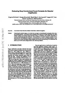
Agfa_DC-504_0 Agfa_DC-733s_0 Agfa_DC-830i_0 Agfa_Sensor505-x_0 Agfa_Sensor530s_0 Canon_Ixus55_0 Canon_Ixus70_0 Canon_Ixus70_1 Canon_Ixus70_2 Canon_PowerShotA640_0 Casio_EX-Z150_0 Casio_EX-Z150_1 Casio_EX-Z150_2 Casio_EX-Z150_3 Casio_EX-Z150_4 FujiFilm_FinePixJ50_0 FujiFilm_FinePixJ50_1 FujiFilm_FinePixJ50_2 Kodak_M1063_0 Kodak_M1063_1 Kodak_M1063_2 Kodak_M1063_3 Kodak_M1063_4 Nikon_CoolPixS710_0 Nikon_CoolPixS710_1 Nikon_CoolPixS710_2 Nikon_CoolPixS710_3 Nikon_CoolPixS710_4 Nikon_D200_0 Nikon_D200_1 Nikon_D70_0 Nikon_D70_1 Nikon_D70s_0 Nikon_D70s_1 Olympus_mju_1050SW_0 Olympus_mju_1050SW_1 Olympus_mju_1050SW_2 Olympus_mju_1050SW_3 Olympus_mju_1050SW_4 Panasonic_DMC-FZ50_0 Panasonic_DMC-FZ50_1 Panasonic_DMC-FZ50_2 Pentax_OptioA40_0 Pentax_OptioA40_1 Pentax_OptioA40_2 Pentax_OptioA40_3 Pentax_OptioW60_0 Praktica_DCZ5.9_0 Praktica_DCZ5.9_1 Praktica_DCZ5.9_2 Praktica_DCZ5.9_3 Praktica_DCZ5.9_4 Ricoh_GX100_0 Ricoh_GX100_1 Ricoh_GX100_2 Ricoh_GX100_3 Ricoh_GX100_4 Rollei_RCP-7325XS_0 Rollei_RCP-7325XS_1 Rollei_RCP-7325XS_2 Samsung_L74wide_0 Samsung_L74wide_1 Samsung_L74wide_2 Samsung_NV15_0 Samsung_NV15_1 Samsung_NV15_2 Sony_DSC-H50_0 Sony_DSC-H50_1 Sony_DSC-T77_0 Sony_DSC-T77_1 Sony_DSC-T77_2 Sony_DSC-T77_3 Sony_DSC-W170_0 Sony_DSC-W170_1

Fig. 1. Confusion matrix for the instance-level camera identification tasks. Different instances of the same model are denoted with a different number at the end of their names. The algorithm tends to confuse pictures belonging to the same camera models. 4.1. Instance-level camera identification

1. For the instance-level (model-level) identification task, we divided the images in several bins, according to the particular instance (model) of camera that acquired the images; 2. For each bin, we assigned approximately 70% of the images to the training set, and the remaining 30% to the test set; 3. We extracted 25 patches from each image, and we assign them to either the training or the test set, according to the split done at the previous step; 4. We build a ground truth by assigning each patch to the corresponding camera instance/model. The ground truth consists of 74 and 27 possible labels for the instance- and model-level identification task, respectively. At the end of this procedure, we end up with a dataset consisting of approximately 415k patches, 300k belonging to the training set and 115k to the test set. Notice that, thanks to our fair procedure, patches used for training do not belong to images used for testing. To implement the convolutional neural network presented in Section 3, we resorted to the MatConvNet library [24]. For both tasks, we trained the network for 200 epochs. The workstation used for the training stage features a quad-core 2.4GHz Intel Xeon CPU E5-2609, a NVIDIA GTX980 GPU and 32GB of RAM. The training process took approximately 3 days to complete. A decreasing learning rate and the dropout layer prevented most of the overfitting during the training process.

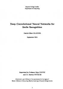
Figure 1 shows the confusion matrix obtained on the test set. The overall accuracy on the test set is equal to 0.298. As shown by the confusion matrix, the intra-model confusion is quite large. In fact, it is possible to identify clear clusters corresponding to camera models, and the performance is quite good in the case of a single instance of the same camera model, whereas it significantly degrades when there are multiple cameras belonging to the same model. Despite being quite complex, such model based on small image patches is not sufficiently powerful to identify the traces of a particular camera instances, like the Photo Response Non-Uniformity (PRNU). Instead, it is quite clear that it is able to recognize some patterns left by the particular camera model. The next section further explores the model-level camera identification task. 4.2. Model-level camera identification Figure 2 shows the confusion matrix for the model-level camera identification task. As shown by the confusion matrix, the model is quite good at discriminating between different models. The precision for this task is as high as 0.729. Furthermore, it is possible to note that it is still difficult to distinguish slightly different models, belonging to the same brand. For instance, Nikon D70 and Nikon D70s are quite difficult to be distinguished, and the same happens for Sony cameras. To further improve the performance, it is possible to use multiple patches as input, aggregating their output to obtain a single prediction. In particular, each patch is fed to the ConvNet, that processes

overall accuracy: 72.99% Agfa_DC-504 Agfa_DC-733s Agfa_DC-830i Agfa_Sensor505-x Agfa_Sensor530s Canon_Ixus55 Canon_Ixus70 Canon_PowerShotA640 Casio_EX-Z150 FujiFilm_FinePixJ50 Kodak_M1063 Nikon_CoolPixS710 Nikon_D200 Nikon_D70_ Nikon_D70s Olympus_mju_1050SW Panasonic_DMC-FZ50 Pentax_OptioA40 Pentax_OptioW60 Praktica_DCZ5.9 Ricoh_GX100 Rollei_RCP-7325XS Samsung_L74wide Samsung_NV15 Sony_DSC-H50 Sony_DSC-T77 Sony_DSC-W170

Fig. 4. The filters learned at the first level of the ConvNet. Some filters look like color contrast/edge detector whereas others resemble some regular interpolation patterns.

Fig. 2. Confusion matrix for the model-level camera identification tasks. Only a few camera models of the same vendor are sometimes confused (i.e., Sony and NikonD70/70s). 0.95

0.9

accuracy

0.85

0.8

Fig. 5. The feature maps obtained at the output of the first convolutional layer.

0.75

0.7 0

5

10

15

20

# patches

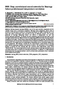
Fig. 3. The accuracy for the model-level identification task as a function of the number of voting patches. Using 20 patches per images grants 94% accuracy in 100ms of computational time. it to give the predicted model label as output. A single label is obtained aggregating the result by means of majority voting. That is, each patch votes for a camera model, and the model that receives the most votes is the final prediction. Figure 3 shows the accuracy of the final model as a function of the number of patches used as input. As can be imagined, the more patches are used, the better the results in terms of accuracy. When 5 patches are used, the accuracy performance is just below 0.90, whereas from 10 patches onwards the accuracy value tends to saturate. When 20 patches are used, the best performance is recorded, with an accuracy value corresponding to 0.941. This value means that the model is able to assign an input image to the correct model, among 27 possible choices, almost 19 times out of 20. Despite being complex, the model is computationally efficient. In fact, less than 100ms are needed to extract features from a batch of 20 patches and obtain the predicted camera model label. 4.3. What does the model learn? Since the model performs well with respect to the model-level identification task, it would be interesting to understand what are the

patterns identified by the convolutional network. Figure 4 shows the filters that are learned at the first convolutional layer of the network, whereas Figure 5 shows the output of such filters. Some filters look like edge and color contrast detectors or low-pass filters, while some others look like quite complex intensity interpolation patterns. It is reasonable to assume that such filters identify some patterns that are characteristic of the acquisition and processing pipeline of a given camera model (e.g., CFA interpolation algorithms, lens-aberration correction methods, etc.). 5. CONCLUSIONS We presented a method for identifying camera instances and models starting from simple image patches, based on deep convolutional networks. The presented model consists of a series of simple operations like filtering, spatial pooling and non-linear activation. The precision of the model is quite high in the case of model-level camera identification, ranging from 0.729 when a single patch is used, to 0.941 in the case of 20 input patches whose output is aggregated by means of majority voting. Instead, the model is not sufficiently complex to effectively distinguish between instances of the same model. Future work includes a more thorough investigation of instancelevel camera identification, with the aim of reducing the intra-model ambiguity, and the development of deep learning models to identify the single operations within an image processing chain, including resizing, interpolation and image compression. Additionally, future work will be devoted to the development of open-set classification algorithms that enable to understand whether a picture belongs to a camera in our dataset or not.

6. REFERENCES [1] A. Piva, “An overview on image forensics,” ISRN Signal Processing, vol. 2013, pp. 22, 2013.

[13] A. Cortiana, V. Conotter, G. Boato, and F. De Natale, “Performance comparison of denoising filters for source camera identification,” in SPIE Conference on Media Watermarking, Security, and Forensics, 2011.

[2] A. Rocha, W. Scheirer, T. Boult, and S. Goldenstein, “Vision of the unseen: Current trends and challenges in digital image and video forensics,” ACM Computing Surveys (CSUR), vol. 43, pp. 26:1–26:42, 2011.

[14] G. Chierchia, D. Cozzolino, G. Poggi, C. Sansone, and L. Verdoliva, “Guided filtering for PRNU-based localization of small-size image forgeries,” in IEEE International Conference on Acoustics, Speech and Signal Processing (ICASSP), 2014.

[3] S. Bayram, H. Sencar, N. Memon, and I. Avcibas, “Source camera identification based on CFA interpolation,” in IEEE International Conference on Image Processing (ICIP), 2005.

[15] L. Gaborini, P. Bestagini, S. Milani, M. Tagliasacchi, and S. Tubaro, “Multi-clue image tampering localization,” in IEEE International Workshop on Information Forensics and Security (WIFS), 2014.

[4] S. Milani, P. Bestagini, M. Tagliasacchi, and S. Tubaro, “Demosaicing strategy identification via eigenalgorithms,” in IEEE International Conference on Acoustics, Speech and Signal Processing (ICASSP), 2014. [5] S.-H. Chen and C.-T. Hsu, “Source camera identification based on camera gain histogram,” in IEEE International Conference on Image Processing (ICIP), 2007. [6] K. Choi, E. Lam, and K. Wong, “Automatic source camera identification using the intrinsic lens radial distortion,” Optics Express, vol. 14, pp. 11551–11565, 2006. [7] Z. Deng, A. Gijsenij, and J. Zhang, “Source camera identification using auto-white balance approximation,” in IEEE International Conference on Computer Vision (ICCV), 2011. [8] A. Dirik, H. Sencar, and N. Memon, “Digital single lens reflex camera identification from traces of sensor dust,” IEEE Transactions on Information Forensics and Security (TIFS), vol. 3, pp. 539–552, 2008. [9] J. Luk´asˇ, J. Fridrich, and M. Goljan, “Determining digital image origin using sensor imperfections,” in IS&T/SPIE Electronic Imaging (EI), 2005. [10] J. Luk´asˇ, J. Fridrich, and M. Goljan, “Digital camera identification from sensor pattern noise,” IEEE Transactions on Information Forensics and Security (TIFS), vol. 1, pp. 205–214, 2006. [11] M. Goljan, J. Fridrich, and T. Filler, “Large scale test of sensor fingerprint camera identification,” in IS&T/SPIE Electronic Imaging (EI), 2009. [12] I. Amerini, R. Caldelli, V. Cappellini, F. Picchioni, and A. Piva, “Estimate of PRNU noise based on different noise models for source camera identification,” International Journal of Digital Crime and Forensics, vol. 2, pp. 21–33, 2010.

[16] M. Buccoli, P. Bestagini, M. Zanoni, A. Sarti, and S. Tubaro, “Unsupervised feature learning for bootleg detection using deep learning architectures,” in IEEE International Workshop on Information Forensics and Security (WIFS), 2014. [17] D. Luo, R. Yang, and J. Huang, “Detecting double compressed AMR audio using deep learning,” in IEEE International Conference on Acoustics, Speech and Signal Processing (ICASSP), May 2014, pp. 2669–2673. [18] C. Jiansheng, K. Xiangui, L. Ye, and Z. J. Wang, “Median filtering forensics based on convolutional neural networks,” IEEE Signal Processing Letters (SPL), vol. 22, pp. 1849–1853, 2015. [19] Y. LeCun and Y. Bengio, “The handbook of brain theory and neural networks,” chapter Convolutional Networks for Images, Speech, and Time Series, pp. 255–258. MIT Press, 1998. [20] Y. Bengio, “Learning Deep Architectures for AI,” Foundations and Trends in Machine Learning, vol. 2, pp. 1–127, 2009. [21] T. Gloe and R. B¨ohme, “The Dresden image database for benchmarking digital image forensics,” Journal of Digital Forensic Practice, vol. 3, pp. 150–159, 2010. [22] V. Nair and G. Hinton, “Rectified linear units improve restricted boltzmann machines,” in International Conference on Machine Learning (ICML), 2010. [23] N. Srivastava, G. Hinton, A. Krizhevsky, I. Sutskever, and R. Salakhutdinov, “Dropout: A simple way to prevent neural networks from overfitting,” Journal of Machine Learning Research, vol. 15, pp. 1929–1958, 2014. [24] A. Vedaldi and K. Lenc, “MatConvNet - convolutional neural networks for MATLAB,” in ACM International Conference on Multimedia (ACM-MM), 2015.