works for resale or redistribution to servers or lists, or to reuse any copyrighted component of this work in other .... Subsections 2.1 and 2.2 are dedicated to value.
Can Program Profiling Support Value Prediction? Freddy Gabbay and Avi Mendelson Department of Electrical Engineering Technion - Israel Institute of Technology, Haifa 32000, Israel. {fredg@psl, mendlson@ee}.technion.ac.il
Copyright 1997 IEEE. Published in the Proceedings of Micro-30, December 1-3, 1997 in Research Triangle Park, North Carolina. Personal use of this material is permitted. However, permission to reprint/republish this material for advertising or promotional purposes or for creating new collective works for resale or redistribution to servers or lists, or to reuse any copyrighted component of this work in other works, must be obtained from the IEEE. Contact: Manager, Copyrights and Permissions IEEE Service Center 445 Hoes Lane P.O. Box 1331 Piscataway, NJ 08855-1331, USA. Telephone: + Intl. 908-562-3966.
Can Program Profiling Support Value Prediction? Freddy Gabbay and Avi Mendelson Department of Electrical Engineering Technion - Israel Institute of Technology, Haifa 32000, Israel. {fredg@psl, mendlson@ee}.technion.ac.il Abstract This paper explores the possibility of using program profiling to enhance the efficiency of value prediction. Value prediction attempts to eliminate true-data dependencies by predicting the outcome values of instructions at run-time and executing true-data dependent instructions based on that prediction. So far, all published papers in this area have examined hardware-only value prediction mechanisms. In order to enhance the efficiency of value prediction, it is proposed to employ program profiling to collect information that describes the tendency of instructions in a program to be value-predictable. The compiler that acts as a mediator can pass this information to the value-prediction hardware mechanisms. Such information can be exploited by the hardware in order to reduce mispredictions, better utilize the prediction table resources, distinguish between different value predictability patterns and still benefit from the advantages of value prediction to increase instruction-level parallelism. We show that our new method outperforms the hardware-only mechanisms in most of the examined benchmarks.
1. Introduction Modern microprocessor architectures are increasingly designed to employ multiple execution units that are capable of executing several instructions (retrieved from a sequential instruction stream) in parallel. The efficiency of such architectures is highly dependent on the instruction-level parallelism (ILP) that they can extract from a program. The extractable ILP depends on both processor’s hardware mechanisms as well as the program’s characteristics ([6], [7]). Program’s characteristics affect the ILP in the sense that instructions cannot always be eligible for parallel execution due to several constraints. These constraints have been classified into three classes: true-data dependencies, name dependencies (false dependencies) and control dependencies ([6], [7], [15]). Both control dependencies and name dependencies are not
considered an upper bound on the extractable ILP since they can be handled or even eliminated in several cases by various hardware and software techniques ([1], [2], [3], [6], [7], [8], [13], [14], [16], [17]). As opposed to name dependencies and control dependencies, only true-data dependencies were considered to be a fundamental limit on the extractable ILP since they reflect the serial nature of a program by dictating in which sequence data should be passed between instructions. This kind of extractable parallelism is represented by the dataflow graph of the program ([7]). Recent works ([9], [10], [4], [5]) have proposed a novel hardware-based paradigm that allows superscalar processors to exceed the limits of true-data dependencies. This paradigm, termed value prediction, attempted to collapse true-data dependencies by predicting at run-time the outcome values of instructions and executing the true-data dependent instructions based on that prediction. Within this concept, it has been shown that the limits of true-data dependencies can be exceeded without violating the sequential program correctness. This claim breaks two accepted fundamental principles: 1. the ILP of a sequential program is limited by its dataflow graph representation, and 2. in order to guarantee the correct execution of the program, true-data dependent instructions cannot be executed in parallel. It was also indicated that value prediction can cause the execution of instructions to become speculative. Unlike branch prediction that can also cause instructions to be executed speculatively since they are control dependent, value prediction may cause instructions to become speculative since it is not assured that they were fed with the correct input values. All recent works in the area of value prediction considered hardware-only mechanisms. In this paper we provide new opportunities enabling the compiler to support value prediction by using program profiling. Profiling techniques are being widely used in different compilation areas to enhance the optimization of programs. In general, the idea of profiling is to study the behavior of the program based on its previous runs. In each of the past runs, the program can be executed based on different sets of input
parameters and input files (training inputs). During these runs, the required information (profile image) can be collected. Once this information is available it can be used by the compiler to optimize the program’s code more efficiently. The efficiency of program profiling is mainly based on the assumption that the characteristics of the program remain the same under different runs as well. In this paper we address several new open questions regarding the potential of profiling and the compiler to support value prediction. Note that we do not attempt to replace all the value prediction hardware mechanisms in the compiler or the profiler. We aim at revising certain parts of the value prediction mechanisms to exploit information that is collected by the profiler. In the profile phase, we suggest collecting information about the instructions’ tendency to be value-predictable (value predictability) and classify them accordingly (e.g., we can detect the highly predictable instructions and the unpredictable ones). Classifying instructions according to their value predictability patterns may allow us to avoid the unpredictable instructions from being candidates for value prediction. In general, this capability introduces several significant advantages. First, it allows us to better utilize the prediction table by enabling the allocation of highly predictable instructions only. In addition, in certain microprocessors, mispredicted values may cause some extra misprediction penalty due to their pipeline organization. Therefore the classification allows the processor to reduce the number of mispredictions and saves the extra penalty. Finally, the classification increases the effective prediction accuracy of the predictor. So far, previous works have performed the classification by employing a special hardware mechanism that studies the tendency of instructions to be predictable at run-time ([9], [10], [4], [5]). Such a mechanism is capable of eliminating a significant part of the mispredictions. However, since the classification was performed at run-time, it could not allocate in advance the predictable instructions in the prediction table. As a result unpredictable instructions could have uselessly occupied entries in the prediction table and evacuated the predictable instructions. In this work we propose an alternative technique to perform the classification. We show that profiling can provide the compiler with accurate information about the tendency of instructions to be value-predictable. The role of the compiler in this case is to act as a mediator and to pass the profiling information to the value prediction hardware mechanisms through special opcode directives. We show that such a classification methodology outperforms the hardware-based classification in most of the examined benchmarks. In particular, the performance improvement is most observable when the pressure on the prediction table, in term of potential instructions to be allocated, is high.
Moreover, we indicate that the new classification method introduces better utilization of the prediction table resources and avoidance of value mispredictions. The rest of this paper is organized as follows: Section 2 summarizes previous works and results in the area of value prediction. Section 3 presents the motivation and the methodology of this work. Section 4 explores the potential of program profiling through various quantitative measurements. Section 5 examines the performance gain of the new technique. Section 6 concludes this paper.
2. Previous works and results This section summarizes some of the experimental results and the hardware mechanisms of the previous familiar works in the area of value prediction ([9], [10], [4], [5]). These results and their significance have been broadly studied by these works, however we have chosen to summarize them since they provide substantial motivation to our current work. Subsections 2.1 and 2.2 are dedicated to value prediction mechanisms: value predictors and classification mechanisms. Subsection 2.3, 2.4 and 2.5 describe the statistical characteristics of the phenomena related to value prediction. The relevance of these characteristics to this work is presented in Section 3.
2. 1.Value predictors Previous works have introduced two different hardware-based value predictors: the last-value predictor and the stride predictor. For simplicity, it was assumed that the predictors only predict destination values of register operands, even though these schemes could be generalized and applied to memory storage operands, special registers, the program counter and condition codes. Last-value predictor: ([9], [10]) predicts the destination value of an individual instruction based on the last previously seen value it has generated (or computed). The predictor is organized as a table (e.g., cache table - see figure 2.1), and every entry is uniquely associated with an individual instruction. Each entry contains two fields: tag and last-value. The tag field holds the address of the instruction or part of it (high-order bits in case of an associative cache table), and the last-value field holds the previously seen destination value of the corresponding instruction. In order to obtain the predicted destination value of a given instruction, the table is searched by the absolute address of the instruction. Stride predictor: ([4], [5]) predicts the destination value of an individual instruction based on its last previously seen value and a calculated stride. The predicted value is the sum of the last value and the stride. Each entry in this predictor holds an additional field, termed stride
field that stores the previously seen stride of an individual instruction (figure 2.1). The stride field value is always determined upon the subtraction of two recent consecutive destination values. Last-value predictor Tag
Last value
Stride predictor Last Tag value Stride
. . .
Tag Index Instruction address
. . .
Predicted value ? =
hit/miss
+
Tag Index Instruction address
Predicted value ? =
hit/miss
Figure 2.1 - The “last value” and the “stride” predictors.
2. 2.Classification of value predictability Classification of value predictability aims at distinguishing between instructions which are likely to be correctly predicted and those which tend to be incorrectly predicted by the predictor. A possible method of classifying instructions is using a set of saturated counters ([9], [10]). An individual saturated counter is assigned to each entry in the prediction table. At each occurrence of a successful or unsuccessful prediction the corresponding counter is incremented or decremented respectively. According to the present state of the saturated counter, the processor can decide whether to take the suggested prediction or to avoid it. In Section 5 we compare the effectiveness of this hardware-based classification mechanism versus the proposed mechanism.
2. 3.Value prediction accuracy The benefit of using value prediction is significantly dependent on the accuracy that the value predictor can accomplish. The previous works in this field ([4], [5], [9] and [10]) provided substantial evidence to support the observation that outcome values in programs tend to be predictable (value predictability). The prediction accuracy measurements of the predictors that were described in Subsection 2.1 on Spec-95 benchmarks are summarized in table 2.1. Note that in the floating point benchmarks (Spec-fp95) the prediction accuracy was measured in each benchmark for two execution phases: initialization (when the program reads its input data) and computation (when
the actual computation is made). Broad study and analysis of these measurements can be found in [4] and [5]. Prediction accuracy [%] Integer ALU FP loads FP loads instructions computation instructions benchmark S L S L S L S L Spec-int95 48 50 61 53 Spec-fp95 70 66 52 47 Init. phase Spec-fp95 63 37 96 23 46 44 29 28 Comp. phase Notations Last-value predictor S Stride predictor L Table 2.1 - Value prediction accuracy measurements.
2. 4.Distribution of value prediction accuracy Our previous studies ([4], [5]) revealed that the tendency of instruction to be value-predictable does not spread uniformly among the instructions in a program (we only refer to those instructions that assign outcome value to a destination register). Approximately 30% of the instructions are very likely to be correctly predicted with prediction accuracy greater than 90%. In addition, approximately 40% of the instructions are very unlikely to be correctly predicted (with a prediction accuracy less than 10%). This observation is illustrated by figure 2.2 for both integer and floating point benchmarks. The importance of this observation and its implication are discussed in Subsection 3.1.
2. 5.Distribution of non-zero strides In our previous works ([4], [5]) we examined how efficiently the stride predictor takes advantage of the additional “stride” field (in its prediction table) beyond the last-value predictor that only maintains a single field (per entry) of the “last value”. We considered the stride fields to be utilized efficiently only when the predictor accomplishes a correct value prediction and the stride field is not equal to zero (non-zero stride). In order to grade this efficiency we used a measure that we term stride efficiency ratio (measured in percentages). The stride efficiency ratio is the ratio of successful non-zero stride-based value predictions to overall successful predictions.
1. The initialization phase of the floating-point benchmarks is denoted by #1 and the computation phase by #2. 2. gcc1 and gcc2 denotes the measurements when the benchmark was run with different input files (the same for perl1 and perl2).
� �RI�LQV WUXFWLRQV
����
� �RI�LQV WUXFWLRQV
7KH�GLV WULEXWLRQ�RI�SUHGLFWLRQ�DFFXUDF\�
����
���
���
���
���
���
���
���
��� ��
�� JR 63(& ,17��
7KH�GLV WULEXWLRQ�RI�SUHGLFWLRQ�DFFXUDF\�
P��NVL P
JFF�
3UHGLFWLRQ�DFFXUDF\�
JFF� �
FRPSUH OL LMSHJ SHUO� VV �� �� �� �� �� �� ��
SHUO�
YRUWH[
63(& )3��
��
��
WRPFDW WRPFDW VZ LP� VZ LP� VX�FRU VX�FRU K\GUR� K\GUR� PJULG DYJ�� DYJ�� Y�� Y�� � � �� �� G�� G�� D
3UHGLFWLRQ�DFFXUDF\�
�
��
��
��
��
��
��
��
��
��
Figure 2.2 - The spread of instructions according to their value prediction accuracy. Our measurements indicated that in the integer benchmarks the stride efficiency ratio is approximately 16%, and in the floating point benchmarks it varies from 12% in the initialization phase to 43% in the computation phase. We also examined the stride efficiency ratio of each instruction in the program that was allocated to the prediction table. We observed that most of these instructions could be divided into two major subsets: a small subset of instructions which always exhibits a relatively high stride efficiency ratio and a large subset of instructions which always tend to reuse their last value (with a very low stride efficiency ratio). Figure 2.3 draws histograms of our experiments and illustrates how instructions in the program are scattered according to their stride efficiency ratio. % of instructions
Stride efficiency ratio
100%
100
80%
90 80
60%
70 60
40%
50 40
20%
30 20
0% 099.go 124.m88k 126.gcc 129.comp sim ress
130.li
132.ijpeg 134.perl 147.vorte 107.mgrid x
10
Figure 2.3 - The spread of instructions according to their stride efficiency ratio.
3. The proposed methodology Profiling techniques are broadly being employed in various compilation areas to enhance the optimization of programs. The principle of this technique is to study the behavior of the program based on one set of train inputs and to provide the gathered information to the compiler. The effectiveness of this technique relies on the assumption that the behavioral characteristics of the program remain consistent with other program’s runs as well. In the first subsection we present how the previous knowledge in the area of value prediction motivated us towards our new approach. In the second subsection we present our methodology and its main principles.
3. 1.Motivation The consequences of the previous results described in Section 2 are very significant, since they establish the basis and motivation for our current work with respect to the following aspects: 1. The measurements described in Subsection 2.3 indicated that a considerable portion of the values that are computed by programs tends to be predictable (either by stride or last-value predictors). It was shown in the previous works that exploiting this property allows the processor to exceed the dataflow graph limits and improve ILP. 2. Our measurements in Subsection 2.4 indicated that the tendency of instructions to be value predictable does not spread uniformly among the instructions in the program. In fact, most programs exhibit two sets of instructions, highly value-predictable instructions and highly unpredictable ones. This observation established the basis for emlpoying classification mechanisms. 3. Previous experiments ([4], [5]) have also provided preliminary indication that different input files do not dramatically affect the prediction accuracy of several examined benchmarks. If this observation is found to be common enough, then it may have a tremendous significance when considering the involvement of program profiling. It may imply that the profiling information which is collected in previous runs of the program (running the application with training input files) can be correlated to the true situation where the program runs with its real input files (provided by the user). This property is extensively examined in this paper. 4. We have also indicated that the set of value-predictable instructions in the program is partitioned into two subsets: a small subset of instructions that exhibit stride value predictability (predictable only by the stride predictor) and a large subset of instructions which tend to reuse their last value (predictable by both predictors). Our previous works ([4], [5]) showed that although the first subset is relatively smaller than the second subset, it appears frequently enough to significantly affect the extractable ILP. On one hand, if we only use the last-value predictor then it cannot
exploit the predictability of the first subset of instructions. On the other hand, if we only use the stride predictor, then in a significant number of entries in the prediction table, the extra stride field is useless because it is assigned to instructions that tend to reuse their most recently produced value (zero strides). This observation motivates us to employ a hybrid predictor that combines both the stride prediction table and the last-value prediction table. For instance we may consider a relatively small stride prediction table only for the instructions that exhibit stride patterns and a larger table for the instructions that tend to reproduce their last value. The combination of these schemes may allow us utilize the extra stride field more efficiently.
3. 2. A classification based on program profiling and compiler support The methodology that we are introducing in this work combines both program profiling and compiler support to perform the classification of instructions according to their tendency to be value predictable. All familiar previous works performed the classification by using a hardware mechanism that studies the tendency of instructions to be predictable at run-time ([4], [5], [9], [10]). Such a mechanism was capable of eliminating a significant part of the mispredictions. However, since the classification was performed dynamically, it could not allocate in advance the highly value predictable instructions in the prediction table. As a result unpredictable instructions could have uselessly occupied entries in the prediction table and evacuated useful instructions. The alternative classification technique, proposed in this paper, has two tasks: 1. identify the highly predictable instructions and 2. indicate whether an instruction is likely to repeat its last value or whether it exhibits stride patterns. Our methodology consists of three basic phases (figure 3.1). In the first phase the program is ordinarily compiled (the compiler can use all the available and known optimization methods) and the code is generated. In the second phase the profile image of the program is collected. The profile image describes the prediction accuracy of each instruction in the program (we only refer to instructions which write a computed value to a destination register). In order to collect this information, the program can be run on a simulation environment (e.g., the SHADE simulator - see [12]) where the simulator can emulate the operation of the value predictor and measure for each instruction its prediction accuracy. If the simulation emulates the operation of the stride predictor it can also measure the stride efficiency ratio of each instruction. Such profiling information could not only indicate which instructions tend to be value-predictable or not, but also which ones exhibit value predictability patterns in form of
“strides” or “last-value”. The output of the profile phase can be a file that is organized as a table. Each entry is associated with an individual instruction and consists of three fields: the instruction’s address, its prediction accuracy and its stride efficiency ratio. Note that in the profile phase the program can be run either single or multiple times, where in each run the program is driven by different input parameters and files. Phase #1
Phase #2
Phase #3 New binary executable with opcode directives
Simulator
Compiler
Train input parameters and files Compiler
Program (C or FORTRAN)
Binary executable
Profile image file
threshold value (user)
Figure 3.1 - The three phases of the proposed classification methodology. In the final phase the compiler only inserts directives in the opcode of instructions. It does not perform instruction scheduling or any form of code movement with respect to the code that was generated in the first phase. The inserted directives act as hints about the value predictability of instructions that are supplied to the hardware. Note, that we consider such use of opcode directives as feasible, since recent processors, such as the PowerPC 601, made branch predictions based on opcode directives too ([11]). Our compiler employs two kinds of directives: the “stride” and the “last-value”. The “stride” directive indicates that the instruction tends to exhibit stride patterns, and the “last-value” directive indicates that the instruction is likely to repeat its recently generated outcome value. By default, if none of these directives are inserted in the opcode, the instruction is not recommended to be value predicted. The compiler can determine which instructions are inserted with the special directives according to the profile image file and a threshold value supplied by the user. This value determines the prediction accuracy threshold of instructions to be tagged with a directive as value-predictable. For instance, if the user sets the threshold value to 90%, all the instructions in the profile image file that had a prediction accuracy less than 90% are not inserted with directives (marked as unlikely to be correctly predicted) and all those with prediction accuracy greater than or equal to 90% are marked as predictable. When an instruction is marked as value-predictable, the type of the directive (either “stride” or “last-value”) still needs to be determined. This can be done by examining the stride efficiency ratio that is provided in the profile image
file. A possible heuristic that the compiler can employ is: If the stride efficiency ratio is greater than 50% it indicates that the majority of the correct predictions were non-zero strides and therefore the instruction should be marked as “stride”; otherwise it is tagged with the “last-value” directive. Another way to determine the directive type is to ask the user to supply the threshold value for the stride efficiency ratio. Once this process is completed, the previous hardware-based classification mechanism (the set of saturated counters) becomes unnecessary. Moreover, we can use a hybrid value predictor that consists of two prediction tables: the “last-value” and the “stride” prediction tables (Subsection 2.2). A candidate instruction for value prediction can be allocated to one of these tables according to its opcode directive type. These new capabilities allow us to exploit both value predictability patterns (stride and last-value) and utilize the prediction tables more efficiently. In addition, they allow us to detect in advance the highly predictable instructions, and thus we could reduce the probability that unlikely to be correctly predicted instructions evacuate useful instructions from the prediction table. In order to clarify the principles of our new technique we are assisted by the following sample C program segment:
IRU�[ ���[���������[�� �$>[@ %>[@�&>[@� The program sums the values of two vectors, B and C, into vector A. In the first phase, the compilation of the program with the gcc 2.7.2 compiler (using the “-O2” optimization) yields the following assembly code (for a Sun-Sparc machine on SunOS 4.1.3): (1) OG�>�L���J�@��O� (2) OG�>�L���J�@��L� (3) DGG��L���[���L� (4) DGG��O���L���O� (5) VW���O��>�L���J�@ (6) FPS��L���L� (7) DGG��L���[���L� (8) EFV��[IIIIIII�� (9) DGG��L���[���L�
��/RDG�%>L@ ��/RDG�&>M@ ��,QFUHPHQW�LQGH[�M ��$>N@ %>L@�&>M@ ��6WRUH�$>N@ ��&RPSDUH�LQGH[�M ��,QFUHPHQW�LQGH[�L ��%UDQFK�WR��� ��,QFUHPHQW�LQGH[�N �LQ�WKH�GHOD\�VORW
In the second phase we collect the profile image of the program. A sample output file of this process is illustrated by table 3.1. It can be seen that this table includes all the instructions in the program that assign values to a destination register (load and add instructions). For simplicity, we only refer to value prediction where the destination operand is a register. However our
methodology is not limited by any means to being applied when the destination operand is a condition code, a program counter, a memory storage location or a special register. Instruction Prediction Stride efficiency address accuracy ratio 1 10% 2% 2 40% 1% 3 99.99% 99.99% 4 20% 1% 7 99.99% 99.99% 9 99.99% 99.99% Table 3.1 - A sample profile image output. In this example the profile image indicates that the prediction accuracy of the instructions that compute the index of the loop was 99.99% and their efficiency ratio was 99.99%. Such an observation is reasonable since the destination value of these instructions can be correctly predicted by the stride predictor. The other instructions in our example accomplished relatively low prediction accuracy and stride efficiency ratio. If the user determines the prediction accuracy threshold to be 90%, then in the third phase the compiler would modify the opcodes of the add operations in addresses 3, 7, and 9 and insert into these opcodes the “stride” directive. All other instructions in the program are unaffected.
4. Examining the potential of profiling through quantitative measurements This section is dedicated to examining the basic question: can program profiling supply the value prediction hardware mechanisms with accurate information about the tendency of instructions to be value-predictable? In order to answer this question, we need to explore whether programs exhibit similar patterns when they are being run with different input parameters. If under different runs of the programs these patterns are correlated, this confirms our claim that profiling can supply accurate information. For our experiments we use different programs, chosen from the Spec95 benchmarks (table 4.1), with different input parameters and input files. In order to collect the profile image we traced the execution of the programs by the SHADE simulator ([12]) on Sun-Sparc processor. In the first phase, all benchmarks were compiled with the gcc 2.7.2 compiler with all available optimizations.
SPEC95 Benchmarks Description Game playing. A simulator for the 88100 processor. A C compiler based on GNU C 2.5.3. Data compression program using adaptive Lempel-Ziv coding. Lisp interpreter. JPEG encoder. Anagram search program. A single-user object-oriented database transaction benchmark. Multi-grid solver in computing a three dimensional potential field. Table 4.1 - Spec95 benchmarks.
mi = max{| v1,i − v 2, i |,| v1, i − v3, i |,
Benchmarks go m88ksim gcc compress95 li ijpeg perl vortex mgrid
For each run of a program we create a profile image containing statistical information that was collected during run-time. The profile image of each run can be regarded as a vector V , where each of its coordinates represents the value prediction accuracy of an individual instruction (the dimension of the vector is determined by the number of different instructions that were traced during the experiment). As a result of running the same program n times, each time with different input parameters and input files, we obtain a set of n vectors V = {V1 , V2 ,...,Vn } where
(
the vector V j = v j,1 , v j,2 ,
�,
v j,k
)
represents the
profile image of run j. Note that in each run we may collect statistical information of instructions which may not appear in other runs. Therefore, we only consider the instructions that appear in all the different runs of the program. Instructions which only appear in certain runs are omitted from the vectors (our measurements indicate that the number of these instructions is relatively small). By omitting these instructions we can organize the components of each vector such that corresponding coordinates would refer to the prediction accuracy of same instruction, i.e., the set of coordinates {v1,l , v 2,l ,..., v n,l } refers to the prediction accuracy of the same instruction l under the different runs of the program. Our first goal is to evaluate the correlation between the tendencies of instructions to be value-predictable under different runs of a program with different input files and parameters. Therefore, once the set of vectors V = {V1 , V2 ,..., Vn } is collected, we need to define a certain metric for measuring the similarity (or the correlation) between them. We choose to use two metrics to measure the resemblance between the vectors. We term the first metric the maximum-distance metric. This metric is a M (V ) max = (m1 , m2 , , mk ) vector whose
�
coordinates are calculated as illustrated by equation 4.1:
| v 2, i − v 3, i |,| v 2, i − v 4, i
�
�,| v |, �| v
1, i
− v n, i |,
2, i
− v n, i |,
| v( n − 1), i − v n, i |} Equation 4.1 - The Mmax metric. Each coordinate of M(V)max is equal to the maximum distance between the corresponding coordinates of each pair of vectors from the set V = {V1 , V2 ,..., Vn } . The second metric that we use is less strict. We term this metric the average-distance metric. This metric is also a vector, M (V ) average = (m1 , m2 , , mk ) , where each of its
�
coordinates is equal to the arithmetic-average distance between the corresponding coordinates of each pair of vectors from the set V = {V1 , V2 ,..., Vn } (equation 4.2). mi = average arith {| v1,i − v 2,i |,| v 1,i − v 3,i |, | v 2 ,i − v 3,i |,| v 2 ,i − v 4,i |,
�
�| v
�,| v
2 ,i
1,i
− v n ,i |,
− v n ,i |,
| v ( n −1 ),i − v n ,i |}
Equation 4.2 - The Maverage metric. Obviously, one can use other metrics in order to measure the similarity between the vectors, e.g., instead of taking the arithmetic average we could take the geometric average. However, we think that these metrics sufficiently satisfy our needs. Once our metrics are calculated out of the profile image, we can illustrate the distribution of its coordinates by building a histogram. For instance, we can count the number of M(V)max coordinates whose values are in each of the intervals: [0,10], (10,20], (30,40], ...,(90,100]. If we observe that most of the coordinates are scattered in the lower intervals, we can conclude that our measurements are similar and that the correlation between the vectors is very high. Figures 4.1 and 4.2 illustrate such histograms for our two metrics M(V)max and M(V)average respectively. 100%
The spread of the coordinates of M(V)max 100
80%
90 80 70
60%
60 50
40%
40 30
20%
20 10
0%
n=5
099.go 124.m88 126.gcc 129.com ksim press
130.li
132.ijpeg 134.perl 147.vorte 107.mgri x d
Figure 4.1 - The spread of M(V)max.
The spread of the coordinates of M(V)average
100%
100%
The spread of the coordinate of M(S)average 100
100 90
80%
90 80
80%
80 70
60%
70
60%
60 50
60 50
40%
40%
40
40 30
20%
30
20%
20 10
20 10
0% 099.go 124.m88 126.gcc 129.com ksim press
n=5
130.li
132.ijpeg 134.perl 147.vorte 107.mgri x d
Figure 4.2 - The spread of M(V)average. In these histograms we clearly observe that in all the benchmarks most of the coordinates are spread across the lower intervals. This observation provides the first substantial evidence that confirms one of our main claims the tendency of instructions in a program to be value predictable is independent of the program’s input parameters and data. In addition it confirms our claim that program profiling can supply accurate information about the tendency of instructions to be value predictable. As we have previously indicated, the profile image of the program that is provided to the compiler can be better tuned so that it can indicate which instructions tend to repeat their recently generated value and which tend to exhibit patterns of strides. In order to evaluate the potential of such classification we need to explore whether the set of instructions whose outcome values exhibit tendency of strides is common to the different runs of the program. This can be done by examining the stride efficiency ratio of each instruction in the program from the profile image file. In this case, we obtain from the profile image file a vector S , where each of its coordinates represents the stride efficiency ratio of an individual instruction. When we run the same program n times (each time with different input parameters and input files) we obtain a set of n vectors S = {S1 , S 2 ,..., S n } where the vector
(
S j = s j,1 , s j,2 ,
�,
s j,k
)
represents the profile image
of run j. Once these vectors are collected we can use one of the previous metrics either the maximum-distance or the average-distance in order to measure the resemblance between the set of vectors S = {S1 , S 2 ,..., S n } . For simplicity we have chosen this time only the average-distance metric to demonstrate the resemblance between the vectors. Once this metric is calculated out of the profile information, we obtain a vector M(S)average. Similar to our previous analysis, we draw a histogram to illustrate the distribution of the coordinates of M(S)average (figure 4.3).
0%
n=5
099.go 124.m88ks 126.gcc 129.compr 130.li im ess
132.ijpeg 134.perl 147.vortex107.mgrid
Figure 4.3 - The spread of M(S)average. Again in this histogram we clearly observe that in all the benchmarks most of the coordinates are spread across the lower intervals. This observation provides evidence that confirms our claim that the set of instructions in the program that tend to exhibit value predictability patterns in form of stride is independent of the program’s input parameters and data. Therefore profiling can accurately detect these instructions and provide this information to the compiler.
5. The effect of the profiling-based classification on value-prediction performance In this section we focus on three main aspects: 1. the classification accuracy of our mechanism, 2. its potential to better utilize the prediction table entries and 3. its effect on the extractable ILP when using value prediction. We also compare our new technique versus the hardware only classification mechanism (saturated counters).
5. 1.The classification accuracy The quality of the classification process can be represented by the classification accuracy, i.e., the fraction of correct classifications out of overall prediction attempts. We measured the classification accuracy of our new mechanism and compared it to the hardware-based mechanism. The classification accuracy was measured for the incorrect and correct predictions separately (using the “stride” predictor), as illustrated by figures 5.1 and 5.2 respectively. Note that these two cases represent a fundamental trade-off in the classification operation since improving the classification accuracy of the incorrect predictions can reduce the classification accuracy of the correct predictions and vice versa. Our measurements currently isolate the effect of the prediction table size since in this subsection we wish to focus only on the pure potential of the proposed technique to successfully classify either correct or incorrect value predictions. Hence, we assume that each of the classification mechanisms has an infinite prediction table (a stride predictor), and that the hardware-based
classification mechanism also maintains an infinite set of saturated counters. The effect of the finite prediction table is presented in the next subsection. The precentages of the mispredictions which are classified correctly 100 80 60 40 20 0 go FSM
m88ksim gcc Prof th=90%
compress Prof th=80%
li
ijpeg Prof th=70%
perl
vortex
Prof th=60%
mgrid average Prof th=50%
Figure 5.1 - The percentages of the mispredictions which are classified correctly. The percentages of the correct predictions which are classified correctly 100 80 60 40 20 0 go m88ksim gcc compress li ijpeg perl vortex mgrid average FSM Prof th=90% Prof th=80% Prof th=70% Prof th=60% Prof th=50%
Figure 5.2 - The percentages of the correct predictions which are classified correctly. Our observations indicate that in most cases the profiling-based classification better eliminates mispredictions in comparison with the saturated counters. When the threshold value of our classification mechanism is reduced, the classification accuracy of mispredictions decreases as well, since the classification becomes less strict. Only when the threshold value is less than 60% does the hardware-based classification gain better classification accuracy for the mispredictions than our proposed mechanism (on the average). Decreasing the threshold value of our classification mechanisms improves the detection of the correct predictions at the expense of the detection of mispredictions. Figure 5.2 indicates that in most cases the hardware-based classification achieves slightly better classification accuracy of correct predictions in comparison with the profiling-based classification. Notice that this observation does not imply at all that the hardware-based classification outperforms the profiling-based classification, because the effect of the table size was not included in these measurements. 5. 2.The effect on the prediction table utilization We have already indicated that when using the hardware-based classification mechanism, unpredictable
instructions may uselessly occupy entries in the prediction table and can purge out highly predictable instructions. As a result, the efficiency of the predictor can be decreased, as well as the utilization of the table and the prediction accuracy. Our classification mechanism can overcome this drawback, since it is capable of detecting the highly predictable instructions in advance, and hence decreasing the pollution of the table caused by unpredictable instructions. In table 5.1 we show the fraction (in percentages) of potential candidates which are allowed to be allocated in the table by our classification mechanism out of those allocated by the saturated counters. It can be observed that even with a threshold value of 50%, the new mechanism can reduce the number of potential candidates by nearly 50%. Moreover, this number can be reduced even more significantly when the threshold is tightened, e.g., a threshold value of 90% reduces the number of potential candidates by more than 75%. This unique capability of our mechanism allows us to use a smaller prediction table and utilize it more efficiently. Profiling threshold 90% 80% 70% 60% 50% The fraction of potential 24% 32% 35% 39% 47% candidates to be allocated relative to those in the saturated counters Table 5.1 - The fraction of potential candidates to be allocated relative to those in the hardware-based classification. In order to evaluate the performance gain of our classification method in comparison with the hardware-based classification mechanism, we measured both the total number of correct predictions and the total number of mispredictions when the table size is finite. The predictor, used in our experiments, is the “stride predictor”, which was organized as a 512-entry, 2-way set associative table. In addition, in the case of the profiling-based classification, instructions were allowed to be allocated to the prediction table only when they were tagged with either the “last-value” or the “stride” directives. Our results, summarized in figures 5.3 and 5.4, illustrate the increase in the number of correct predictions and incorrect predictions respectively gained by the new mechanism (relative to the saturated counters). It can be observed that the profiling threshold plays the main role in the tuning of our new mechanism. By choosing the right threshold, we can tune our mechanism in such way that it outperforms the hardware-based classification mechanism in most benchmarks. In the benchmarks go, gcc, li, perl and vortex, we can accomplish both a significant increase in the number of correct predictions and a reduction in the number of mispredictions. For instance, when using a
threshold value in the range of 80-90% in vortex, our mechanism accomplishes both more correct predictions and less incorrect predictions than the hardware-only mechanism. Similar achievements are also obtained in go when the range of threshold values is 60-90%, in gcc when the range is 70-90%, in li when the threshold value is 60% and in perl when the range is 70-90%. In the other benchmarks (m88ksim, compress, ijpeg and mgrid) we cannot find a threshold value that yields both an increase in the total number of correct predictions and a decrease in the number of mispredictions. The explanation of this observation is that these benchmarks employ relatively much smaller working-sets of instructions and therefore they can much less exploit the benefits of our classification mechanism. Also notice that the mispredictions increase, observed for our classification mechanism in m88ksim, is not expected to significantly affect the extractable ILP, since the prediction accuracy of this benchmark is already very high. ,QFUHDVH�LQ�WKH�QXPEHU�RI�FRUUHFW�SUHGLFWLRQV
��� ���
with a finite instruction window of 40 entries, unlimited number of execution units and a perfect branch prediction mechanism. In addition, the type of value predictor that we use and its table organization are the same as in the previous subsection. In case of value-misprediction, the penalty in our abstract machine is 1 clock cycle. Notice that such a machine model can explore the pure potential of the examined mechanisms without being constrained by individual machine limitations. Our experimental results, summarized in table 5.2, present the increase in ILP gained by using value prediction under different classification mechanisms (relative to the case when value prediction is not used). In most benchmarks we observe that our mechanism can be tuned, by choosing the right threshold value, such that it can achieve better results than those gained by the saturated counters. In addition, we also observe that when decreasing the threshold value from 90% to 50% the ILP gained by our new mechanism increases (in most cases). The explanation of this phenomenon is that in our range of threshold values, the contribution of increasing the correct predictions (as a result of decreasing the threshold) is more significant than the effect of increasing mispredictions.
���
�� ����
ILP increase VP + VP + VP + VP + VP + Prof. Prof. Prof. Prof. Prof. 90% 80% 70% 60% 50% 10% 9% 10% 13% 13% 13% 593% 489% 492% 565% 577% 577% 15% 16% 17% 21% 21% 21% 11% 7% 7% 8% 8% 8% 37% 33% 35% 38% 38% 40% 16% 14% 14% 15% 16% 15% 19% 23% 24% 28% 28% 27% 159% 175% 178% 180% 179% 179% 24% 7% 10% 11% 11% 11%
Benchmark VP + SC
���� ���� JR
P��NVL
JFF
FRPSUH
P 3URI��WK
��
OL
LMSHJ
��
3URI��WK
SHUO
YRUWH[
PJULG
VV
3URI��WK
��
3URI��WK
��
3URI��WK
��
Figure 5.3 - The increase in the total number of correct predictions. ,QFUHDVH�LQ�WKH�QXPEHU�RI�LQFRUUHFW�SUHGLFWLRQV ����
����
����
����
��
����� JR
P��NVL
JFF
P 3URI��WK
��
3URI��WK
FRPSU
OL
LMSHJ
��
3URI��WK
SHUO
YRUWH[
PJULG
HVV ��
3URI��WK
��
3URI��WK
��
Figure 5.4 - The increase in the total number of incorrect predictions.
5. 3.The effect of the classification on the extractable ILP In this subsection we examine the ILP that can be extracted by value prediction under different classification mechanisms. Our experiments consider an abstract machine
go m88ksim gcc compress li ijpeg perl vortex mgrid
Notations VP + SC Value prediction using saturated counters. VP + Prof. Value prediction using the profiling-based X% classification and a threshold value = X%. Table 5.2 - The increase in ILP under different classification mechanisms relative to the case when value prediction is not used.
6. Conclusions This paper introduced a profiling-based technique to enhance the efficiency of value prediction mechanisms. The new approach suggests using program profiling in order to classify instructions according to their tendency to be value-predictable. The collected information by the
profiler is supplied to the value prediction mechanisms through special directives inserted into the opcode of instructions. We have shown that the profiling information which is extracted from previous runs of a program with one set of input parameters is highly correlated with the future runs under other sets of inputs. This observation is very important, since it reveals various opportunities to involve the compiler in the prediction process and thus to increase the accuracy and the efficiency of the value predictor. Our experiments also indicated that the profiling information can distinguish between different value predictability patterns (such as “last-value” or “stride”). As a result, we can use a hybrid value predictor that consists of two prediction tables: the last-value and the stride prediction tables. A candidate instruction for value prediction can be allocated to one of these tables according to its profiling classification. This capability allows us to exploit both value predictability patterns (stride and last-value) and utilize the prediction tables more efficiently. Our performance analysis showed that the profiling-based mechanism could be tuned by choosing the right threshold value so that it outperformed the hardware-only mechanism in most benchmarks. In many benchmarks we could accomplish both a significant increase in the number of correct predictions and a reduction in the number of mispredictions. The innovation in this paper is very important for future integration of the compiler with value prediction. We are currently working on other properties of the program that can be identified by the profiler to enhance the performance and the effectiveness of value prediction. We are examining the effect of the profiling information on the scheduling of instruction within a basic block and the analysis of the critical path. In addition, we also explore the effect of different programming styles such as object oriented on the value predictability patters.
References [1] S. Davidson, D. Landskov, B. D. Shriver and P. W. Mallet. Some Experiments in Local Microcode Compaction for Horizontal Machines. IEEE Transactions on Computers, Vol. C-30, no. 7, July, 1981, pp. 460-477. [2] J. R. Ellis. Bulldog: A Compiler for VLIW Architecture. MIT Press, Cambridge, Mass., 1986. [3] J. A. Fisher. The Optimization of Horizontal Microcode Within and Beyond Basic Blocks: An Application of Processor Scheduling with Resources. Ph.D. dissertation, TR COO-3077-161. Courant Mathematics and Computing Laboratory, New York University, NY, October, 1979. [4] F. Gabbay and A. Mendelson. Speculative Execution based on Value Prediction. EE Department TR #1080, Technion Israel Institute of Technology, November, 1996.
[5] F. Gabbay and A. Mendelson. An Experimental and Analytical Study of Speculative Execution based on Value Prediction. Submitted to publication to the IEEE Transactions on Computer Systems, June, 1997. EE Department TR #1124, Technion - Israel Institute of Technology, June., 1997. [6] J. L. Hennessy and D. A. Patterson. Computer Architecture a Quantitative Approach. Morgan Kaufman Publishers, Inc., Second edition, 1995. [7] M. Johnson. Superscalar Microprocessor Design. Prentice Hall, Englewood Cliffs, 1990, N.J. [8] M. S. Lam. Software Pipelining: An Effective Scheduling Technique for VLIW Processors. Proc. of the SIGPLAN’88 Conference on Programming Languages Design and Implementation, ACM. June, 1988, pp. 318-328. [9] M. H. Lipasti, C. B. Wilkerson and J. P. Shen. Value Locality and Load Value Prediction. Proc. of the 7th International Conference on Architectural Support for Programming Languages and Operating Systems (ASPLOSVII), Oct., 1996. [10] M. H. Lipasti and J. P. Shen. Exceeding the Dataflow Limit via Value Prediction. Proc. of the 29th Annual ACM/IEEE International Symposium on Microarchitecture, December, 1996. [11] Motorola, PoerwPC 601 User’s Manual. 1993, No. MPC601UM/AD. [12] Introduction to Shade, Sun Microsystems Laboratories, Inc. TR 415-960-1300, Revision A of 1/Apr/92. [13] A. Smith and J. Lee. Branch Prediction Strategies and Branch-Target Buffer Design. Computer 17:1, January, 1984. pp. 6-22. [14] J. E. Smith. A Study of Branch Prediction Techniques. Proc. of the 8th International Symposium on Computer Architecture, June, 1981. [15] D. W. Wall. Limits of Instruction-Level Parallelism. Proc. of the 4th Conference on Architectural Support for Programming Languages and Operating Systems. Apr., 1991. pp. 248-259. [16] S. Weiss and J. E. Smith. A Study of Scalar Compilation Techniques for Pipelined Supercomputers. Proc. of the 2nd International Conference on Architectural Support for Programming Languages and Operating Systems. October, 1987, pp. 105-109. [17] T. Y. Yeh and Y. N. Patt. Alternative Implementations of Two-Level Adaptive Branch Prediction. Proc. of the 19th International Symposium on Computer Architecture. May, 1992. pp. 124-134.