Gomory's fractional cutting plane method and of two heuristics mimick- ... On the other hand, pure cutting plane methods based on Gomory cuts alone are.
Can pure cutting plane algorithms work? Arrigo Zanette1 , Matteo Fischetti1? and Egon Balas2?? 1
2
DEI, University of Padova Carnegie Mellon University, Pittsburgh, PA
Abstract. We discuss an implementation of the lexicographic version of Gomory’s fractional cutting plane method and of two heuristics mimicking the latter. In computational testing on a battery of MIPLIB problems we compare the performance of these variants with that of the standard Gomory algorithm, both in the single-cut and in the multi-cut (rounds of cuts) version, and show that they provide a radical improvement over the standard procedure. In particular, we report the exact solution of ILP instances from MIPLIB such as stein15, stein27, and bm23, for which the standard Gomory cutting plane algorithm is not able to close more than a tiny fraction of the integrality gap. We also offer an explanation for this surprizing phenomenon. Keywords: Cutting Plane Methods, Gomory Cuts, Degeneracy in Linear Programming, Lexicographic Dual Simplex, Computational Analysis.
1
Introduction
Modern branch-and-cut methods for (mixed or pure) Integer Linear Programs are heavily based on general-purpose cutting planes such as Gomory cuts, that are used to reduce the number of branching nodes needed to reach optimality. On the other hand, pure cutting plane methods based on Gomory cuts alone are typically not used in practice, due to their poor convergence properties. In a sense, branching can be viewed as just a “symptomatic cure” to the well-known drawbacks of Gomory cuts—saturation, bad numerical behavior, etc. From the cutting plane point of view, however, the cure is even worse than the disease, in that it hides the real source of the troubles. So, a “theoretically convergent” method such as the Gomory one becomes ancillary to enumeration, and no attempt is made to try to push it to its limits. In this respect, it is instructive to observe that a main piece of information about the performance of Gomory cuts (namely, that they perform much better if generated in rounds) ?
??
The work of the first two authors was supported by the Future and Emerging Technologies unit of the EC (IST priority), under contract no. FP6-021235-2 (project “ARRIVAL”) and by MiUR, Italy (PRIN 2006 project “Models and algorithms for robust network optimization”). The work of the third author was supported by National Science Foundation grant ]DMI-0352885 and Office of Naval Research contract ]N00014-03-1-0133
2
Arrigo Zanette, Matteo Fischetti and Egon Balas
was discovered only in 1996 (Balas, Ceria, Cornu´ejols, and Natraj [2]), i.e., about 40 years after their introduction [7]. The purpose of our project, whose scope extends well beyond the present paper, is to try to come up with a viable pure cutting plane method (i.e., one that is not knocked out by numerical difficulties), even if on most problems it will not be competitive with the branch-and-bound based methods. As a first step, we chose to test our ideas on Gomory’s fractional cuts, for two reasons: they are the simplest to generate, and they have the property that when expressed in the structural variables, all their coefficients are integer (which makes it easier to work with them and to assess how nice or weird they are). In particular, we addressed the following questions: i) Given an ILP, which is the most effective way to generate fractional Gomory cuts from the optimal LP tableaux so as to push the LP bound as close as possible to the optimal integer value? ii) What is the role of degeneracy in Gomory’s method? iii) How can we try to counteract the numerical instability associated with the iterated use of Gomory cuts? iv) Is the classical polyhedral paradigm “the stronger the cut, the better” still applicable in the context of Gomory cuts read from the tableau? The question is not at all naive, as one has to take into account the negative effects that a stronger yet denser (or numerically less accurate) cut has in the next tableaux, and hence in the next cuts. As we were in the process of testing various ways of keeping the basis determinant and/or condition number within reasonable limits, our youngest coauthor had the idea of implementing the lexicographic dual simplex algorithm used in one of Gomory’s two finite convergence proofs. Gomory himself never advocated the practical use of this method; on the contrary, he stressed that its sole purpose was to simplify one of the two proofs, and that in practice other choice criteria in the pivoting sequence were likely to work better. Actually, we have no information on anybody ever having tried extensively this method in practice. The lexicographic method has two basic ingredients: (a) the starting tableau is not just optimal, i.e., dual feasible, but lexicographically dual-feasible, and the method of reoptimization after adding a cut is the lexicographic dual simplex method; and (b) at least after every k iterations for some fixed k, the row with the first fractional basic variable is chosen as source row for the next cut. The implementation of this method produced a huge surprise: the lexicographic method produces a dramatic improvement not only in gap closure (see Figure 1), but also in determinant and cut coefficient size. It is well known that cutting plane methods work better if the cuts are generated in rounds rather than individually (i.e., if cuts from all fractional variables are added before reoptimization, rather than reoptimizing after every cut). Now it seems that if we are generating rounds of cuts rather than individual cuts, the use of the lexicographic rule would make much less sense, in particular because (b) is automatically satisfied—so the lexicographic rule plays a role only
Can pure cutting plane algorithms work? 4
5.564
Air04 (single−cut)
x 10
Stein27 (single−cut) 18
Lex
Lex
17 objective bound
5.562 objective bound
3
5.56
5.558
TB
16 15 14
5.556
TB
13 5.554
0
500
1000 1500 # cuts
2000
0
2000
4000 # cuts
6000
8000
Fig. 1. Comparison between the textbook and lexicographic implementations of single-cut Gomory’s algorithm on air04 and stein27.
in shaping the pivoting sequence in the reoptimization process. So we did not expect it to make much of a difference. Here came our second great surprize: as illustrated in Figure 2, even more strikingly than when using single cuts, comparing the standard and lexicographic methods with rounds of cuts shows a huge difference not only in terms of gap closed (which for the lexicographic version is 100% for more than half the instances in our testbed), but also of determinant size and coefficient size. 4
5.566
Air04 (multi−cut)
x 10
Stein27 (multi−cut) 18
Lex
Lex 17 objective bound
objective bound
5.564
5.562
TB
5.56
16 15 14
5.558
TB
13 5.556
0
1
2 3 # cuts
4
0 4
x 10
1
2 # cuts
3 4
x 10
Fig. 2. Comparison between the textbook and lexicographic implementations of multi-cut Gomory’s algorithm on air04 and stein27.
In this paper we discuss ad evaluate computationally and implementation of the lexicographic version of Gomory’s fractional cutting plane method and
4
Arrigo Zanette, Matteo Fischetti and Egon Balas
of two heuristics mimicking the latter one, and offer an interpretation of the outcome of our experiments.
2
Gomory cuts
In this paper we focus on pure cutting plane methods applied to solving Integer Linear Programs (ILPs) of the the form: min cT x Ax = b x ≥ 0 integer where A ∈ Zm×n , b ∈ Zm and c ∈ Zn . Let P := {x ∈ LEX (y0 , y1 , . . . , yn ) means that there exists an index k such that xi = yi for all i = 1, . . . , k − 1 and xk > yk . In the lexicographic, as opposed to the usual, dual simplex method the ratio test does not only involve two scalars (reduced cost and pivot candidate) but a column and a scalar. So, its implementation is straightforward, at least in theory. In practice, however, there are a number of major concerns that limit this approach: 1. the ratio test has a worst-case quadratic time complexity in the size of the problem matrix; 2. the ratio test may fail in selecting the right column to preserve lex-optimality, due to round-off errors; 3. the algorithm requires taking control of each single pivot operation, which excludes the possibility of applying much more effective pivot-selection criteria. The last point is maybe the most important. As a clever approach should not interfere too much with the black-box LP solver used, one could think of using a perturbed linear objective function x0 + �1 x1 + �2 x2 . . ., where x0 is the actual objective and 1 � �1 � �2 � . . .. Though this approach is numerically unacceptable, one can mimic it by using the following method which resembles the iterative procedure used in the construction of the so-called Balinsky–Tucker tableau [3] and is akin to the slack fixing used in sequential solution of preemptive linear goal programming (see [1] and [10]). Starting from the optimal solution (x?0 , x?1 , . . . , x?n ), we want to find another basic solution for which x0 = x?0 but x1 < x?1 (if any), by exploiting dual degeneracy. So, we fix the variables that are nonbasic (at their bound) and have a nonzero reduced cost. This fixing implies the fixing of the objective function value to x?0 , but has a major advantage: since we fix only variables at their bounds, the fixed variables will remain out of the basis in all the subsequent
Can pure cutting plane algorithms work?
7
steps. Then we reoptimize the LP by using x1 as the objective function (to be minimized), fix other nonbasic variables, and repeat. The method then keeps optimizing subsequent variables, in lexicographic order, over smaller and smaller dual-degenerate subspaces, until either no degeneracy remains, or all variables are fixed. At this point we can unfix all the fixed variables and restore the original objective function, the lex-optimal basis being associated with the non-fixed variables. This approach proved to be quite effective (and stable) in practice: even for large problems, where the classical algorithm is painfully slow or even fails, our alternative method requires short computing time to convert the optimal basis into a lexicographically-minimal one. We have to admit however that our current implementation is not perfect, as it requires deciding whether a reduced cost is zero or not: in some (rare) cases, numerical errors lead to a wrong decision that does not yield a lexicographically dual-feasible final tableau. We are confident however that a tighter integration with the underlying LP solver could solve most of the difficulties in our present implementation.
4
Heuristics variants
While the lexicographic simplex method gives an exact solution to the problem of degeneracy, simple heuristics can be devised that mimic the behavior of lexicographic dual simplex. The scope of these heuristics is to try to highlight the crucial properties that allow the lexicographic method to produce stable Gomory cuts. As already mentioned, a lex-optimal solution can in principle be reached by using an appropriate perturbation of the objective function, namely x0 + �1 x1 + . . . + �n xn with 1 � �1 � . . . � �n . Although this approach is actually impractical, one can use a 1-level approximation where the perturbation affects a single variable only, say xi , leading to the new objective function min x0 + �xi . The perturbation term is intended to favor the choice of an equivalent optimal basis closer to the lexicographically optimal one, where the chosen variable xi is moved towards its lower bound—and hopefully becomes integer. In our first heuristic, Heur1, when the objective function is degenerate we swap our focus to the candidate cut generating variable, i.e., the variable xi to be perturbed is chosen as the most lex-significant fractional variable. The idea is that each new cut should guarantee a significant lex-decrease in the solution vector by either moving to a new vertex where the cut generating variables becomes integer, or else some other more lex-significant variables becomes fractional and can be cut. A second perturbation heuristic, Heur2, can be designed along the following lines. Consider the addition of a single FGC and the subsequent tableau reoptimization performed by a standard dual simplex method. After the first pivot operation, the slack variable associated with the new cut goes to zero and leaves the basis, and it is unlikely that it will re-enter it in a subsequent step. This however turns out to be undesirable in the long run, since it increases the chances
8
Arrigo Zanette, Matteo Fischetti and Egon Balas
that the FGC generated in the next iterations will involve the slack variables of the previously-generated FGCs, and hence it favors the generation of cuts of higher rank and the propagation of their undesirable characteristics (density, numerical inaccuracy, etc.). By exploiting dual degeneracy, however, one could try to select an equivalent optimal basis that includes the slack variables of the FGCs. This can be achieved by simply giving a small negative cost to the FGC slack variables. Both the heuristics above involve the use of a small perturbation in the objective function coefficients, that however can produce numerical troubles that interfere with our study. So we handled perturbation in a way similar to that used in our implementation of the lexicographic dual simplex, that requires the solution of two LPs—one with the standard objective function, and the second with the second-level objective function and all nonbasic variables having nonzero reduced cost fixed at their bound.
5
Computational results
Our set of pure ILP instances mainly comes from MIPLIB 2003 and MIPLIB 3; see Table 1. It is worth noting that, to our knowledge, even very small instances of these libraries (such as stein15, bm23, etc.) have never been solved by a pure cutting plane method based on FGC or GMI cuts read from the LP tableau. Problem air04 air05 bm23 cap6000 hard ks100 hard ks9 krob200 l152lav lin318 lseu manna81 mitre mzzv11 mzzv42z p0033 p0201 p0548 p2756 pipex protfold sentoy seymour stein15 stein27 timtab
Cons 823 426 20 2176 1 1 200 97 318 28 6480 2054 9499 10460 16 133 176 755 2 2112 30 4944 35 118 171
Vars LP opt Opt Source 8904 55535.44 56137 MIPLIB 3.0 7195 25877.61 26374 MIPLIB 3.0 27 20.57 34 MIPLIB 6000 -2451537.33 -2451377 MIPLIB 3.0 100 -227303.66 -226649 Single knapsack 9 -20112.98 -19516 Single knapsack 19900 27347 27768 2 matching 1989 4656.36 4722 MIPLIB 50403 38963.5 39266 2 matching 89 834.68 1120 MIPLIB 3321 -13297 -13164 MIPLIB 3.0 9958 114740.52 115155 MIPLIB 3.0 10240 -22945.24 -21718 MIPLIB 3.0 11717 -21623 -20540 MIPLIB 3.0 33 2520.57 3089 MIPLIB 201 6875 7615 MIPLIB 3.0 548 315.29 8691 MIPLIB 3.0 2756 2688.75 3124 MIPLIB 3.0 48 773751.06 788263 MIPLIB 1835 -41.96 -31 MIPLIB 3.0 60 -7839.28 -7772 MIPLIB 1372 403.85 423 MIPLIB 3.0 15 5 9 MIPLIB 27 13 18 MIPLIB 3.0 397 28694 764772 MIPLIB 3.0
Table 1. Our test bed
Input data is assumed to be integer. All problems are preprocessed by adding an integer variable x0 that accounts for the original objective function, from
Can pure cutting plane algorithms work?
9
which we can derive valid cuts, as Gomory’s proof of convergence prescribes. Once a FGC is generated, we put it in its all-integer form in the space of the structural variables. In order to control round-off propagation, our FGC separator uses a threshold of 0.1 to test whether a coefficient is integer or not: a coefficient with fractional part smaller than 0.1 is rounded to its nearest integer, whereas cuts with larger fractionalities are viewed as unreliable and hence discarded. We carried out our experiments in a Intel Core 2 Q6600, 2.40GHz, with a time limit of 1 hour of CPU time and a memory limit of 2GB for each instance. Our first set of experiments addressed the single-cut version of Gomory’s algorithm. Actually, at each iteration we decided to generate two FGCs from the selected cut generating row—one from the tableau row itself, and one from the same row multiplied by -1. The choice of the cut generation row in case of the lexicographic method is governed by the rule that prescribes the selection of the least-index variable. As to the other methods under comparison, the cut generation row is chosen with a random policy giving a higher probability of selecting the cut-generating variable from those with fractional part closer to 0.5 (alternative rules produced comparable results). A very important implementation choice concerns the cut purging criterion. The lexicographic algorithm ensures the lexicographic improvement of the solution vector after each reoptimization, thus allowing one to remove cuts as soon as they become slack at the new optimum. As far as other methods are concerned, however, we can safely remove cuts only when the objective function improves. Indeed, if the objective function remains unchanged a removed cut can be generated again in a subsequent iteration, and the entire algorithm can loop—a situation that we actually encountered during our experiments. We therefore decided to remove the slack cuts only when it is mathematically correct, i.e. after a nonzero change in the objective function value, though this policy can lead to an out-of-memory status after a long stalling phase. Table 2 compares results on the textbook implementation of Gomory’s algorithm (TB) and the lexicographic one (Lex). Besides the percentage of closed gap (ClGap), we report 3 tightly correlated parameters to better measure the performance of each method. The first parameter is the cut coefficients size (Coeff.): large coefficients, besides increasing the likelihood of numerical errors, can be a symptom of cut ineffectiveness since they are required to represent very small angles in the space of structural variables. The second parameter is the determinant of the optimal basis (Det.). In a sense, the problem being all-integer, the determinant is a measure of the distance from an integer solution: a unit determinant implies an all-integer tableau and solution. Since any coefficient in the tableau can be expressed as a rational number whose denominator is the determinant of the current basis B, the smallest fractional part we could encounter in a tableau is 1/det(B)—weird tableau entries correspond to large determinants. However, our experiments showed that there are instances with huge determinants (e.g., mitre) but numerically quite stable. This is because the size of the
10
Arrigo Zanette, Matteo Fischetti and Egon Balas
determinant is only a weak bound on the degree of fractionality of the solution, as the large denominator can be – and fortunately often is – compensated by a large numerator. A more reliable indicator of numerical precision loss is our third parameter, the condition number κ of the optimal basis, which gives a measure of the inaccuracy of the finite-precision representation of a solution x to the linear system Bx = b. In the table, only the maximum value of the three indicators above during the run is reported. The first column reports one of the following exit-status codes: (O) integer optimum, (tL) time limit, (cL) limit of 100,000 cuts, (M) out of memory, (E) numerical errors (either no cuts passed the integrality check, or the problem became infeasible), and (lE) if one of the reoptimizations required by the lexicographic method failed for numerical reasons. A possible failure of the lexicographic method arises when a strict lexicographic improvement is not reached because of numerical issues. In these situations we are no longer protected against the TB drawbacks and we can fail. Precisely, in sentoy (single-cut) we failed to improve lexicographically for 27 iterations, in p0548 for 2597 iterations and in timtab1-int for 3 iterations. In multi-cut versions, we failed in sentoy for 5 iterations, p0201 for 57 iterations, in p0548 for 173 iterations, in p2756 for 5 iterations, and in timtab1-int for 5 iterations. Table 2 shows clearly that in most cases the TB version has huge coefficient sizes, determinants and condition numbers, while in Lex all these values remain relatively small along the entire run. Moreover, Lex could solve to proven optimality 9 of the 25 instances of our testbed—some of these instances being notoriously hard for pure cutting plane methods. For illustration purposes, Figure 3 gives a representation of the trajectory of the LP optimal vertices to be cut (along with a plot of the basis determinant) when the textbook and the lexicographic methods are used for instance stein15. In Figures 3(a) and (b), the vertical axis represents the objective function value. As to the XY space, it is a projection of the original 15-dimensional variable space. The projection is obtained by using a standard procedure available e.g. in MATLAB (namely, multidimensional scaling [4]) with the aim of preserving the metric of the original 15-dimensional space as much as possible. In particular, the original Euclidean distances tend to be preserved, so points that look close one to each other in the figure are likely to be also close in the original space. According to Figure 3(a), the textbook method concentrates on cutting points belonging to a small region. This behavior is in a sense a consequence of the efficiency of the underlying LP solver, that has no incentive in changing the LP solution once it becomes optimal with respect to the original objective function—the standard dual simplex will stop as soon as a feasible point (typically very close to the previous optimal vertex) is reached. As new degenerate vertices are created by the cuts themselves, the textbook method enters a feedback loop that is responsible for the exponential growth of the determinant of the current basis, as reported in Figure 3(d).
Can pure cutting plane algorithms work? (b) Lex solutions trajectory
9
9
8
8 objective
objective
(a) TB solutions trajectory
7
7
6
6
5
5
Y
Y
X (c) Part of lex sol. traj. (objective = 8)
11
X (d) Determinant
20
10
TB Lex 15
10
10
Y
10
5
10
0
10 X
0
20
40 # itrs
60
80
Fig. 3. Problem stein15 (single cut). (a)-(b) Solution trajectories for TB and Lex, resp.; (c) Lower dimensional representation of the the Lex solution trajectory; the filled circles are lexicographic optima used for cut separation; their immediate next circles are optima given by the black-box dual-simplex solver, whereas the other points correspond to the equivalent solutions visited during lexicographic reoptimization; the double circle highlights the trajectory starting point. (d) Growth of determinants in TB and Lex (logarithmic scale).
On the contrary, as shown in Figures 3(b), the lexicographic method prevents this by always moving the fractional vertex to be cut as far as possible (in the lex-sense) from the previous one. Note that, in principle, this property does not guarantee that there will be no numerical problems, but the method seems to be work pretty well in practice. Finally, Figure 3(c) offers a closer look at the effect of lexicographic reoptimization. Recall that our implementation of the lexicographic dual simplex method involves a sequence of reoptimizations, each of which produces an alternative optimal vertex possibly different from the previous one. As a result, between two consecutive cuts our method internally traces a trajectory of equivalent solutions, hence in the trajectory plotted in Figure 3(b) we can distinguish between two contributions to the movement of x∗ after the addition of a new cut: the one due to the black-box optimizer, an the one due to lex-reoptimization.
12
Arrigo Zanette, Matteo Fischetti and Egon Balas
Figure 3(c) concentrates on the slice objective=8 of the Lex trajectory. Each lexicographic optimal vertex used for cut separation is depicted as a filled circle. The immediate next point in the trajectory is the optimal vertex found by the standard black-box dual simplex, whereas the next ones are those contributed by the lexicographic reoptimization. The figure shows that lexicographic reoptimization has a significant effect in moving the points to be cut, that in some cases are very far from those returned by the black-box dual simplex. To support the interpretation above even further, we performed the experiment of just restarting the LP solver from scratch after having generated the FGCs, so that it is more likely that a “substantially different” optimal solution is found. This small change had a significant impact on the performance of the textbook method (though not comparable to that derived from the use of the lexicographic method), showing the importance of breaking the correlation of the optimal LP bases. Table 4 reports the results of our two heuristics, Heur1 and Heur2. A comparison with the previous table shows that both heuristics are effective in controlling the coefficient size, determinant, and condition number. The average closed gap is significantly better than in TB, but clearly worse than in Lex. A second set of experiments was carried out on the multi-cut version of Gomory’s algorithm, where cuts are generated in rounds. To be specific, after each LP reoptimization we consider all the tableau rows with fractional basic variable, and generate two FGCs from each row—one from the row itself, and one from the same row multiplied by -1. According to Table 3, the multi-cut version of Lex performed even better than in the single-cut mode: in 13 out of the 26 instances the method reached the optimum. Figures 4 and 5 give some illustrative plots for instance sentoy. The figures clearly show the typical degenerate behavior of TB, with instable phases of rapid growth of determint/coefficients/κ exploring small space regions with shallow cuts. It is worth observing the striking difference in the plots of the average cut depth, computed as the geometric distance of the cut from the separated vertex, averaged over all the cuts in a round. Even more interesting, the TB and Lex have a completely different behavior as far as the optima distance (computed as the Euclidean distance between two consecutive fractional vertices to be cut) is concerned. As a matter of fact, as already shown by Figure 3, lexicographic reoptimization is quite successful in amplifying the dynamic (and diversity) of the fractional solutions.
6
Conclusions and future work
Pure cutting plane algorithms have been found not to work in practice because of numerical problems due to the cuts becoming increasingly parallel (a phenomenon accompanied by dual degeneracy), increasing determinant size and condition number, etc. For these reasons, cutting planes are in practice used in cut-and-branch or branch-and-cut mode.
tL tL M tL O O O tL 0 E O tL tL tL E tL tL tL E tL E tL E E tL
Itrs 1197 2852 5370 1666 3134 1058 281 3412 1667 4115 423 6445 203 195 2919 14521 19279 5834 4719 68 830 124 173 208 10784
Cuts 2394 5704 5628 3329 6237 2107 532 6824 3289 8201 423 12882 406 390 5824 29036 38446 11560 9408 136 1639 246 313 365 21501
Time 3602.85 3601.83 2733.43 3603.51 1586.82 2.74 20.81 3602.10 1155.32 671.27 1338.29 3601.11 3618.53 3617.33 1054.55 3601.16 3601.41 3601.75 24.84 3811.43 15.28 3768.72 2.29 3.59 3603.58
Textbook ClGap Coeff. 4.42 1.4e+04 4.51 3.8e+05 18.09 1e+15 8.47 1.5e+10 100.00 8.7e+05 100.00 8.3e+14 100.00 1.2e+02 13.16 6.1e+03 100.00 1.6e+03 60.75 5.2e+14 100.00 1 59.95 1.5e+08 8.98 4.8e+02 2.77 8.5e+02 71.15 5.8e+14 13.92 2.6e+11 50.11 2.4e+12 78.63 5.5e+12 36.26 7.5e+14 8.76 5.2e+10 3.39 4.3e+14 6.01 4.7e+08 12.39 2.1e+16 0 1.5e+16 11.94 1.7e+13 Det. 1.9e+18 1e+27 3.6e+32 1.2e+21 4.1e+08 6.4e+21 4.9e+07 2.7e+09 1.1e+12 7e+31 4.9e+173 Inf 6.4e+57 8.3e+53 1.8e+29 7.9e+36 Inf Inf 8.1e+26 Inf 2.1e+37 5e+56 Inf Inf Inf
κ 1.8e+13 3e+15 2.7e+18 9.2e+21 1.4e+13 1.8e+28 3.2e+08 1.3e+12 5.4e+11 8.5e+30 4.8e+06 4.2e+18 3.4e+12 9.6e+12 1.1e+31 7.4e+25 3.4e+28 1e+27 3.1e+27 2.1e+17 3e+28 9.1e+20 2.5e+20 7e+21 1.2e+27 tL tL tL O lE tL lE cL tL O tL O O cL
tL tL O tL O O tL O tL O
Itrs 371 1012 713 594 214 889 666 1152 200 13541 81 77 52 25 1961 29950 29199 1787 50000 299 5771 94 65 4298 50000
Cuts 742 2024 1426 1188 428 1778 1280 2278 346 27068 81 154 104 50 3832 58845 58216 3574 99390 598 11541 182 121 8301 99887
Time 3604.92 3604.92 2.40 3604.17 1.10 0.74 3606.81 297.83 3618.80 70.74 3617.72 3621.68 3746.52 3810.13 4.22 792.35 3603.34 2957.59 146.86 3606.09 47.88 3618.15 0.18 45.23 3124.58
Lex ClGap Coeff. 14.56 1e+04 22.44 4.8e+03 100.00 2.4e+02 14.08 2.5e+06 100.00 6.7e+05 100.00 4.8e+04 86.70 2.3e+03 100.00 1.7e+04 57.69 1.2e+02 100.00 2.4e+04 9.77 1 2.05 3.2e+03 7.68 61 5.45 37 100.00 2.3e+03 67.57 2.3e+05 0.03 3.4e+06 0.52 9.1e+02 42.43 1.1e+05 45.26 30 100.00 6.5e+04 11.23 15 100.00 17 100.00 7.2e+02 4.00 1.6e+07 Det. 5.2e+10 1.9e+10 4.7e+10 5.1e+09 6.3e+05 5.5e+06 8.6e+07 1.9e+06 1.1e+12 5.2e+18 1.6e+178 Inf 4.3e+48 7.9e+37 3.5e+17 1.2e+22 2.7e+190 1.1e+278 3e+10 1.3e+30 4.6e+34 1.2e+19 3.6e+02 8.9e+04 6e+250
κ 5.2e+18 3.5e+13 1e+10 4.8e+15 1.5e+14 1.4e+10 1e+17 5.9e+11 2e+14 2.7e+13 4.8e+06 1.9e+16 8.7e+12 3.7e+14 2.9e+16 2.7e+16 2.4e+16 5.4e+15 3.4e+21 2.1e+07 1.5e+16 1.6e+08 1.8e+11 1.2e+06 1.5e+21
Table 2. Comparison between textbook and lexicographic implementation of Gomory’s algorithm (single-cut version)
Problem air04 air05 bm23 cap6000 hard ks100 hard ks9 krob200 l152lav lin318 lseu manna81 mitre mzzv11 mzzv42z p0033 p0201 p0548z p2756 pipex protfold sentoy seymour stein15 stein27 timtab1-int
Can pure cutting plane algorithms work? 13
Arrigo Zanette, Matteo Fischetti and Egon Balas 14
Problem air04 air05 bm23 cap6000 hard ks100 hard ks9 krob200 l152lav lin318 lseu manna81 mitre mzzv11 mzzv42z p0033 p0201 p0548 p2756 pipex protfold sentoy seymour stein15 stein27 timtab1-int M M E tL tL O O M O E O M M M M tL M M M M M tL E E M
Itrs 35 30 144 979 1950 269 44 525 15 149 1 94 33 62 1529 1332 825 740 2929 7 1953 18 116 57 231
Cuts 11912 9648 2168 11693 10770 1678 2017 31177 250 3710 270 30016 17936 14664 23328 55408 35944 19925 49391 5526 34503 11748 3265 2399 73188
Time 1209.41 955.09 9.33 3614.59 3603.03 0.30 153.92 2715.78 12.82 34.35 8.88 1262.24 1735.42 1515.50 2493.35 3602.21 2223.35 2423.48 1921.78 1058.84 2586.38 7517.40 9.50 20.01 585.72
Textbook ClGap Coeff. 11.23 2.4e+03 5.11 7.1e+02 5.28 2.3e+15 10.34 1.4e+09 100.00 5e+04 100.00 7.8e+04 100.00 1.6e+02 40.59 5.3e+03 100.00 7 44.58 1.7e+14 100.00 1 85.52 8.9e+08 38.56 4.9e+02 33.80 3e+06 81.53 1.8e+14 19.32 2e+12 48.98 1.3e+09 78.86 4.5e+12 51.25 1.3e+14 8.76 4.6e+06 18.25 5.1e+14 21.67 3.3e+08 20.92 2.5e+15 0.00 1.7e+15 23.59 1.6e+11 Det. 6.9e+11 4.2e+11 5.5e+30 7e+15 2.2e+05 1.7e+05 1e+06 8e+08 3.4e+07 9.8e+33 5.2e+92 Inf Inf Inf 1.1e+34 2e+34 2.4e+137 Inf 3.3e+27 Inf 5.3e+43 1.3e+159 2.4e+26 2.8e+36 Inf
κ 9.3e+09 4.9e+09 8.7e+24 4.3e+20 1.5e+12 6.9e+09 9.4e+07 1.6e+10 9.7e+05 2e+19 3.7e+06 4.2e+20 2.6e+11 6.5e+14 2.2e+24 2.5e+26 2e+24 1.3e+27 4e+28 5.1e+13 7e+30 1.4e+16 3.2e+28 8.3e+18 2.1e+21 tL tL O E O O O O O O O tL tL tL O E E E O tL O tL O O cL
Lex Itrs Cuts Time ClGap Coeff. Det. κ 150 47995 3606.61 19.21 7.3e+03 2.2e+09 3.9e+11 261 76263 3598.20 14.00 1.5e+03 4.9e+10 9.6e+10 659 8298 1.67 100.00 3.7e+02 4.6e+10 3e+14 966 6769 2110.12 24.66 4.5e+06 5.1e+09 1.6e+15 98 439 0.63 100.00 5e+05 1.5e+04 2.8e+09 139 614 0.12 100.00 3e+04 3.6e+04 2.9e+10 17 282 22.18 100.00 7.2 1e+06 3.7e+04 681 22364 206.82 100.00 1.8e+04 6.7e+05 2.4e+10 19 416 124.27 100.00 17 3.2e+07 1.8e+08 1330 18925 6.62 100.00 9.6e+03 1.2e+14 2.6e+14 2 280 29.58 100.00 1 1.7e+97 3.7e+06 232 20972 3619.30 97.83 6.2e+06 Inf 9.1e+13 61 25542 3739.41 40.60 1.8e+02 2.8e+51 8.5e+11 61 14830 3616.85 25.50 8.5e+02 1e+38 8.7e+12 87 1085 0.14 100.00 4.5e+02 1.6e+13 6e+14 27574 629004 1119.71 74.32 2.3e+05 3.6e+22 7.4e+11 461 27067 131.69 47.50 4.8e+06 7.1e+135 5.5e+14 642 14645 509.72 79.09 2.4e+05 Inf 1.1e+13 50000 488285 188.11 74.18 2.8e+05 8.5e+11 1e+14 159 38714 3607.08 45.26 30 1.5e+32 1e+07 5331 68827 25.85 100.00 7.6e+04 3.2e+34 3.9e+14 87 48339 3610.62 26.89 78 1e+23 3.6e+07 64 676 0.14 100.00 15 2e+02 2.3e+06 3175 37180 19.72 100.00 7.5e+02 1.9e+04 1.9e+05 3165 1000191 841.56 50.76 3.5e+06 Inf 1.7e+16
Table 3. Comparison between textbook and lexicographic implementation of Gomory’s algorithm (multi-cut version)
Problem air04 air05 bm23 cap6000 hard ks100 hard ks9 krob200 l152lav lin318 lseu manna81 mitre mzzv11 mzzv42z p0033 p0201 p0548 p2756 pipex protfold sentoy seymour stein15 stein27 timtab1-int tL tL tL tL O O tL tL M tL O tL tL tL O tL tL tL E tL E tL tL tL cL
Itrs 1886 1355 5760 2024 2212 839 3009 5910 1699 17687 425 6003 69 125 20667 10756 22096 4147 50000 366 1184 201 5592 3798 50000
Cuts 3772 2710 6111 4048 4403 1674 5978 11813 3360 35367 425 12003 138 250 41287 21510 44063 8191 99985 732 2357 401 11145 7595 99997
Heur1 ClGap Coeff. 6.24 7.9e+04 4.11 1.1e+10 25.54 1.7e+15 7.85 2.8e+09 100.00 4.9e+11 100.00 1.6e+05 92.40 1.1e+03 46.68 2.7e+05 66.94 5.6e+03 69.16 7.3e+11 100.00 1 47.89 2.3e+05 4.44 1.7e+02 5.72 3.2e+02 100.00 3.3e+08 21.22 3.6e+09 50.61 1.5e+06 78.63 5.6e+10 47.51 1.4e+08 17.88 4.6 7.85 3.9e+14 6.01 9.1e+02 75.00 1.2e+03 0.00 1.4e+02 16.02 1.3e+07 Det. 6.5e+27 1.6e+51 2.2e+29 6.5e+20 3.3e+21 1.6e+07 1e+16 4.6e+11 1.2e+14 7.7e+32 4.9e+173 Inf Inf 1.2e+65 7.6e+20 4e+32 4.7e+190 Inf 1.8e+19 9.6e+37 2.5e+38 4.6e+26 1.5e+11 1.1e+11 Inf
κ 1.5e+15 4.1e+21 1.7e+20 9.6e+20 1.7e+24 2.5e+11 8.2e+11 6.4e+13 6.1e+12 1.8e+24 4.8e+06 1.6e+14 5.4e+12 2.9e+12 1.8e+19 8.7e+21 1.4e+18 1.1e+21 1.2e+17 9.8e+09 1e+29 1.8e+12 1e+09 1.6e+08 4.3e+18 tL tL tL tL 0 O M tL M tL O tL tL tL tL tL tL tL tL tL tL tL tL tL tL
Itrs 1463 1338 3938 1379 627 162 3051 2071 1002 3805 423 5973 267 247 14143 3689 9523 4623 26620 435 6951 275 4148 3645 21474
Cuts 2926 2676 7876 2757 1251 322 6066 4140 1966 7608 423 11934 532 494 28267 7378 19007 9182 53233 870 13900 548 8293 7290 42946
Time 3601.57 3603.34 3602.32 3605.44 11.10 0.10 3544.19 3604.68 1203.28 3601.04 1328.05 3601.13 3612.87 3601.63 3603.52 3601.73 3603.13 3604.52 3601.96 3610.08 3602.91 3615.12 3602.46 3601.92 3601.19
Heur2 ClGap Coeff. 12.06 1.3e+07 4.51 1.1e+05 25.54 1.1e+04 8.47 4.5e+06 100.00 6.4e+05 100.00 5.4e+05 97.15 7.5e+05 32.97 2e+04 88.43 2.1e+04 47.78 2.5e+05 100.00 1 75.15 3e+06 13.45 8.2e+02 8.96 9.3e+03 94.55 1.3e+08 17.16 7.6e+06 43.19 5.8e+06 77.25 3.8e+04 40.68 1.4e+11 8.76 1.5 22.71 3.3e+06 11.23 17 50.00 4.9e+04 0.00 6 14.50 1.1e+09
Table 4. The two heuristics compared (single-cut version).
Time 3602.45 3630.37 3602.69 3601.36 742.51 0.67 3602.40 3601.22 2760.11 3601.67 1329.69 3601.02 3623.00 3667.32 486.85 3602.02 3601.44 3601.76 650.65 3617.67 116.95 3622.41 3601.33 3601.57 1676.40
Det. 7e+15 8.6e+26 2.1e+15 3.8e+13 5.4e+06 5.1e+05 1.3e+13 8.2e+16 2.1e+13 1.6e+24 4.9e+173 Inf 2.8e+54 1.9e+54 4e+17 3.3e+21 1e+190 Inf 2e+19 2.4e+28 8.6e+30 4.9e+17 1.3e+15 1.9e+05 Inf
κ 5.2e+18 3.5e+13 1e+10 4.8e+15 1.5e+14 1.4e+10 1e+17 5.9e+11 2e+14 2.7e+13 4.8e+06 1.9e+16 8.7e+12 3.7e+14 2.9e+16 2.7e+16 2.4e+16 5.4e+15 3.4e+21 2.1e+07 1.5e+16 1.6e+08 1.8e+11 1.2e+06 1.5e+21
Can pure cutting plane algorithms work? 15
Arrigo Zanette, Matteo Fischetti and Egon Balas 16
Problem air04 air05 bm23 cap6000 hard ks100 hard ks9 krob200 l152lav lin318 lseu manna81 mitre mzzv11 mzzv42z p0033 p0201 p0548 p2756 pipex protfold sentoy seymour stein15 stein27 timtab1-int M M M tL tL O O tL O M O tL tL M O tL tL tL E tL E M M M M
Itrs 30 49 1819 484 150 251 12 627 42 2604 1 148 14 18 40 2087 1401 420 50000 19 118 19 985 283 383
Cuts 10250 15805 8403 7002 672 1641 108 30047 2415 54498 270 47954 10452 6818 460 92066 90042 17108 552448 7886 1712 12084 20707 13587 119945
Time 1287.10 1365.48 3112.35 3605.86 1.24 0.33 3.15 3639.62 563.91 3388.00 8.94 3651.05 5544.73 2613.82 0.06 3612.42 3601.77 3613.50 752.66 3775.30 5.06 3081.48 2133.91 937.55 288.72
Heur1 ClGap Coeff. 10.40 1.4e+04 6.53 3.1e+04 18.09 5e+14 7.23 3.5e+08 100.00 1.2e+04 100.00 5.5e+04 100.00 1.2 46.68 1.4e+09 100.00 1e+02 70.21 2.9e+12 100.00 1 88.90 5.4e+07 29.27 8.9e+03 18.28 2.6e+04 100.00 2.5e+02 51.22 1.1e+09 53.75 4.7e+07 78.86 8e+12 55.44 5.3e+09 27.01 6.9 4.88 5.1e+14 21.67 1.3e+02 75.00 1.9e+03 0.00 39 37.10 6.2e+06 Det. 2.1e+10 4.1e+24 1.7e+29 4e+16 3.3e+04 2.6e+05 1e+06 2.3e+24 4.7e+09 2.1e+32 5.2e+92 Inf 4.9e+73 1.2e+52 1.5e+13 1.8e+26 2.4e+137 Inf 1e+20 6.5e+28 1.3e+36 1.1e+31 1.1e+11 9.8e+06 3.9e+216
κ 1.8e+12 2.1e+11 6.7e+22 3.1e+17 1.8e+10 8.3e+10 1.4e+05 5.4e+15 5.6e+08 4.8e+19 3.7e+06 1.1e+17 4.4e+15 3.4e+13 4.1e+06 8.8e+20 1.9e+16 3.1e+27 1.5e+20 1.2e+09 1.1e+20 1.6e+11 1.5e+09 4.2e+06 3.1e+13 M M M M O O O M O M O tL M M M M M M M tL M M M M M
Itrs 28 26 631 559 810 252 9 106 35 542 1 192 40 74 2060 756 358 283 1530 23 1064 30 505 274 688
Cuts 9075 8288 13800 7511 1642 2010 81 9889 1503 16610 270 27786 15727 17099 37057 26159 24003 14402 30972 8488 20822 16270 13838 13586 197581
Time 511.50 667.99 1933.80 2498.47 28.45 1.18 2.27 1034.03 238.84 1433.12 8.83 3624.63 1699.51 2423.77 3190.24 2476.90 1612.11 1852.05 1608.28 3674.48 2111.59 3494.90 1585.78 936.43 733.33
Heur2 ClGap Coeff. 9.73 2.6e+03 5.11 1.8e+03 25.54 4e+06 9.72 1.5e+08 100.00 3.5e+03 100.00 4.9e+05 100.00 1.2 31.44 6.7e+03 100.00 55 48.48 8e+06 100.00 1 91.56 3.4e+04 34.16 3.5e+02 28.44 1.5e+03 91.03 3e+07 37.57 6.9e+04 46.09 2.7e+04 78.40 4.8e+04 48.98 2.2e+07 8.76 1.4 22.71 7.9e+05 26.89 8.8 50.00 44 0.00 4.7 43.08 1.4e+07
Table 5. The two heuristics compared (multi-cut version).
Det. 2.1e+08 3.5e+10 3.5e+23 8e+14 3e+03 2.7e+08 1e+06 1.1e+10 7.6e+08 5.4e+23 5.2e+92 Inf 2.9e+43 1.4e+41 4.9e+16 1.6e+15 5.1e+133 Inf 1.9e+16 2.6e+24 3.2e+29 2.9e+17 3.7e+05 1.8e+05 8.1e+198
κ 3.9e+11 9.6e+10 3e+14 1.6e+15 2.8e+09 2.9e+10 3.7e+04 2.4e+10 1.8e+08 2.6e+14 3.7e+06 9.1e+13 8.5e+11 8.7e+12 6e+14 7.4e+11 5.5e+14 1.1e+13 1e+14 1e+07 3.9e+14 3.6e+07 2.3e+06 1.9e+05 1.7e+16
Can pure cutting plane algorithms work?
17
Bound −7770 TB Lex
objective bound
−7780 −7790 −7800 −7810 −7820 −7830 −7840
0
1
2
3
4
5
6
# cuts
TB
50
4
x 10 Lex
40
10
10
40
determinant
10
30
10
30
10
20
10 20
10
10
10
10
10
0
10
0
0
0.5
1
1.5
2
2.5
10
3
0
1
2
3
4
5
6
4
4
x 10
40
x 10
12
10
10
10
10
30
10
kappa
8
10 20
10
6
10 10
10
4
10
0
10
2
0
0.5
1
1.5 2 # cuts
2.5
10
3 4
x 10
0
1
2
3 4 # cuts
5
6 4
x 10
Fig. 4. Comparison between the textbook and lexicographic implementations of multi-cut Gomory’s algorithm on sentoy.
18
Arrigo Zanette, Matteo Fischetti and Egon Balas
TB
15
average abs value of coeff
10
10
4
10
10
5
3
10
10
0
10
Lex
5
10
2
0
0.5
1
1.5
2
2.5
10
3
0
1
2
3
4
5
6
4
4
x 10
0
0
10
average cut depth
x 10
10
−5
−5
10
10
−10
−10
10
10
0
0.5
1
1.5
2
2.5
3
0
1
2
3
4
5
6
4
4
optima distance
x 10
x 10
3
3
2.5
2.5
2
2
1.5
1.5
1
1
0.5
0.5
0
0.5
1
1.5
2
2.5
3
0 4
x 10
1
2
3
4
5
6 4
x 10
Fig. 5. Comparison between the textbook and lexicographic implementations of multi-cut Gomory’s algorithm on sentoy
Can pure cutting plane algorithms work?
19
In this paper we have discussed an implementation of the lexicographic version of Gomory’s fractional cutting plane method and of two heuristics mimicking the latter one. In computational testing on a battery of MIPLIB problems, we compared the performance of these variants with that of the standard Gomory algorithm, both in the single-cut and in the multi-cut (rounds of cuts) version, and showed that they provide a radical improvement over the standard procedure. In particular, we reported the exact solution of ILP instances from MIPLIB such as stein15, stein27, and bm23, for which the standard Gomory cutting plane algorithm is not able to close more than a tiny fraction of the integrality gap. The significance of these result suggests that the lexicographic approach can be applied to any cutting plane algorithm—no matter what kind of cuts you add in the step that generates cuts, you may reoptimize using the lexicographic dual simplex method so as to break dual degeneracy in favor of “cleaner” LP bases associated with better primal vertices to cut. We plan to investigate this topic in the near future.
References 1. J. L. Arthur and A. Ravindran. PAGP, a partitioning algorithm for (linear) goal programming problems. ACM Trans. Math. Softw., 6(3):378–386, 1980. 2. E. Balas, S. Ceria, G. Cornu´ejols, and N. Natraj. Gomory cuts revisited. Operations Research Letters, 19:1–9, 1996. 3. M. L. Balinski and A. W. Tucker. Duality theory of linear programs: A constructive approach with applications. SIAM Review, 11(3):347–377, July 1969. 4. I. Borg and P.J.F. Groenen. Modern Multidimensional Scaling: Theory and Applications. Springer, 2005. 5. Balas E. and A. Saxena. Optimizing over the split closure. Mathematical Programming, DOI 10.1007/s10107-006-0049-5, 2006. 6. M. Fischetti and Lodi A. Optimizing over the first Chv´ atal closure. Mathematical Programming B, 110(1):3–20, 2007. 7. R. E. Gomory. Outline of an algorithm for integer solutions to linear programs. Bulletin of the American Society, 64:275–278, 1958. 8. R. E. Gomory. An algorithm for the mixed integer problem. Technical Report RM-2597, The RAND Cooperation, 1960. 9. R. E. Gomory. An algorithm for integer solutions to linear programming. In R. L. Graves and P. Wolfe, editors, Recent Advances in Mathematical Programming, pages 269–302, New York, 1963. McGraw-Hill. 10. M. Tamiz, D. F. Jones, and E. El-Darzi. A review of goal programming and its applications. Annals of Operations Research, (1):39–53, 1995.