Geoscientific Model Development
Open Access
Geosci. Model Dev., 7, 419–432, 2014 www.geosci-model-dev.net/7/419/2014/ doi:10.5194/gmd-7-419-2014 © Author(s) 2014. CC Attribution 3.0 License.
Can sparse proxy data constrain the strength of the Atlantic meridional overturning circulation? T. Kurahashi-Nakamura1 , M. Losch2 , and A. Paul1 1 MARUM
– Center for Marine Environmental Sciences and Faculty of Geosciences, University of Bremen, Bremen, Germany 2 Alfred Wegener Institute for Polar and Marine Research, Bremerhaven, Germany Correspondence to: T. Kurahashi-Nakamura (
[email protected]) Received: 17 July 2013 – Published in Geosci. Model Dev. Discuss.: 20 August 2013 Revised: 10 January 2014 – Accepted: 24 January 2014 – Published: 26 February 2014
Abstract. In a feasibility study, the potential of proxy data for the temperature and salinity during the Last Glacial Maximum (LGM, about 19 000 to 23 000 years before present) in constraining the strength of the Atlantic meridional overturning circulation (AMOC) with a general ocean circulation model was explored. The proxy data were simulated by drawing data from four different model simulations at the ocean sediment core locations of the Multiproxy Approach for the Reconstruction of the Glacial Ocean surface (MARGO) project, and perturbing these data with realistic noise estimates. The results suggest that our method has the potential to provide estimates of the past strength of the AMOC even from sparse data, but in general, paleo-seasurface temperature data without additional prior knowledge about the ocean state during the LGM is not adequate to constrain the model. On the one hand, additional data in the deep-ocean and salinity data are shown to be highly important in estimating the LGM circulation. On the other hand, increasing the amount of surface data alone does not appear to be enough for better estimates. Finally, better initial guesses to start the state estimation procedure would greatly improve the performance of the method. Indeed, with a sufficiently good first guess, just the sea-surface temperature data from the MARGO project promise to be sufficient for reliable estimates of the strength of the AMOC.
1
Introduction
The ocean is an important component of the climate system because of its large storage and transport of heat as well as its strong control on the atmospheric circulation. To understand the dynamics of climate change, it is essential to assess the role of the ocean. Proxy evidence (e.g., Keigwin and Lehman, 1994; Clark et al., 2001; Epica Community Members, 2006) and climate models (e.g., Ganopolski and Rahmstorf, 2001; Stocker and Johnsen, 2003) suggest close links between the temperature in the Atlantic region and variations of the Atlantic meridional overturning circulation (AMOC) and North Atlantic Deep Water (NADW) formation during past climate changes such as Dansgaard–Oeschger and Heinrich events. Associated changes in the ventilation of the deep ocean presumably affected the global climate by reorganizing the cycling of carbon and other nutrients, which in turn led to different concentrations of carbon dioxide (CO2 ) in the atmosphere (e.g., Archer, 1991; Archer et al., 2000; Gildor and Tziperman, 2001; Schulz et al., 2001; KurahashiNakamura et al., 2010). Therefore, proper reconstructions of the AMOC is a key element in understanding the climate dynamics in the past. The Last Glacial Maximum (LGM, 19 000–23 000 years before present; Mix et al., 2001) is one of the most suitable time periods for studying a climate that is very different from the modern one, because the data coverage for the LGM is comparatively good, and the radiative forcings, boundary conditions and climate response are relatively well known (Solomon et al., 2007). Nevertheless, the ocean circulation during the LGM is uncertain to the extent that even the
Published by Copernicus Publications on behalf of the European Geosciences Union.
420
T. Kurahashi-Nakamura et al.: Ocean reconstruction from sparse data
question of whether the strength of the AMOC was larger or smaller in the LGM than in the modern day climate is still open to debate. On the one hand, the information on the past AMOC strength is obtained from paleoceanographic proxy variables (Fischer and Wefer, 1999). For example, a weaker AMOC is inferred by Lynch-Stieglitz et al. (1999a, b) and Lynch-Stieglitz et al. (2006) based on a geostrophic transport estimate for the Florida Current from the oxygen isotope ratio (18 O/16 O) recorded in the fossil shells of benthic foraminifera (often expressed as δ 18 O, that is, the deviation from a standard ratio1 ), by Piotrowski et al. (2005) based on neodymium isotope ratios (143 Nd/144 Nd), and by McManus et al. (2004) and Negre et al. (2010) based on north-to-south gradients of rate-sensitive radiogenic 231 Pa/230 Th isotope ratios (Negre et al. (2010) even argue for a reversal of the abyssal flow during the LGM). In contrast, a stronger AMOC is hypothesized by Yu et al. (1996) and Lippold et al. (2012) also based on 231 Pa/230 Th isotope ratios; by McCave et al. (1995), Manighetti and McCave (1995), and McCave and Hall (2006) based on the grain-size analysis of ocean sediments; and by Curry and Oppo (2005) based on the stable carbon isotope ratios (13 C/12 C, often expressed as δ 13 C2 ) of the dissolved inorganic carbon (DIC) in seawater, and cadmium/calcium trace element ratios (Cd/Ca). Finally, Rutberg and Peacock (2006) interpret glacial δ 13 C of DIC as consistent with a circulation regime similar to today. On the other hand, there are various estimates of the overturning strength during the LGM by different numerical climate models. In spite of the same forcing and boundary conditions applied to the models, the estimates with coupled atmosphere–ocean models are not consistent (cf. OttoBliesner et al., 2007). Using inverse methods and data assimilation in the context of the LGM often required simplified ocean models (e.g., Legrand and Wunsch, 1995; Gebbie and Huybers, 2006; Huybers et al., 2007; Burke et al., 2011). For example, Huybers et al. (2007) used a geostrophic model to suggest that reliable estimates of the LGM AMOC requires an accuracy of density data that exceeds that of available data by one order of magnitude. Instead, Huybers et al. propose using conservative tracers such as δ 13 C of DIC for constraining the circulation. There are, however, very few LGM-state estimates based on general circulation models and the adjoint technique. Winguth et al. (1999) and Winguth et al. (2000) assimilated the δ 13 C of DIC and Cd/Ca data into a global ocean model and suggested shallower and about 30 % weaker AMOC strength with an adjoint ocean model (Winguth et al., 2000). Dail (2012) used the sea-surface temperature (SST) 1 It
is
defined
(18 O/16 O)sample −(18 O/16 O)standard × 103 (18 O/16 O)standard 2 It is defined (13 C/12 C)sample −(13 C/12 C)standard × 103 (13 C/12 C)standard
Geosci. Model Dev., 7, 419–432, 2014
as
δ 18 O(‰) =
as
δ 13 C(‰) =
data by the MARGO project (MARGO Project Members, 2009), δ 13 C of DIC, and δ 18 O of seawater for state estimation in the Atlantic domain, and inferred that the NADW in the LGM was shallower but as strong as in the modern day. More direct indicators of the past AMOC strength would be the temperature and salinity of seawater. Since they drive the ocean circulation through density differences, a numerical ocean model could be used to quantify an ocean circulation that is consistent with the temperature and salinity data. To date, the most comprehensive compilation of SST estimates for the LGM ocean is provided by the MARGO project (MARGO Project Members, 2009). A similar data set for sea-surface salinity does not yet exist. Local estimates of the salinity of LGM bottom water may be obtained from measurements of the δ 18 O of the pore fluid in sea-floor sediments (Adkins et al., 2002), but there is no direct proxy for salinity that could be applied generally. The δ 18 O of calcite shells of planktonic foraminifera fossils depend on the local salinity as well as on temperature, and thus it is possible to estimate the salinity if one can remove the temperature effect with the help of an independent temperature proxy such as the Mg/Ca ratio (Gebbie and Huybers, 2006). However, error propagation yields large errors on the reconstructed salinity (Schmidt, 1999; Rohling, 2000). The MARGO project has also assessed the spatial distribution of the available paleo-data for the deep ocean, such as the δ 18 O of benthic foraminifera (Paul and Mulitza, 2009). By all means, the paleo-data coverage is still very sparse compared to the present-day data coverage. Therefore, a powerful data assimilation technique is required to control the model efficiently, given the limited amount of data (Paul and Schäfer-Neth, 2005). In this study, we adopted the constrained least-squares technique for that purpose; namely, we seek a model ocean that corresponds to the minimum value of a so-called objective function, which is mainly the sum of squared differences between data and corresponding model results. This optimized model ocean provides the best estimate for the AMOC strength. The adjoint method (e.g., Wunsch, 1996; Errico, 1997) is a technique to find such an optimized state, because it allows for the computation of the gradient of the objective function with respect to selected control variables (that may include initial and boundary conditions as well as internal model parameters) and search for its minimum. Our ultimate goal is to assimilate various paleo-data for the LGM into a numerical ocean model (Paul and Schäfer-Neth, 2005; Schmittner et al., 2011), with the aim of estimating the LGM ocean state as reliably as possible. As the first step, the particular purpose of this paper is to examine whether the spatial distribution and accuracy of the available compilation of paleo-temperature data is likely to be adequate enough to constrain our model properly, and if not, what further data would be required. For this purpose, we used artificial pseudo-proxy data instead of the actual LGM data and estimated the AMOC strength of a target model ocean from www.geosci-model-dev.net/7/419/2014/
T. Kurahashi-Nakamura et al.: Ocean reconstruction from sparse data which the pseudo-data was sampled. Thus, we could assess the result of our state estimate exercise by comparing the estimated value with the known “true” value. The artificial targets had a stronger or weaker AMOC strength than the reference state to serve as potential analogues for the LGM ocean. The basic set of pseudo-proxy data had the same spatial distribution and error estimates as the MARGO data, in order to imitate the quality and quantity of actual paleo-data. The experiments described in this paper are not identical twin experiments where varied parameters are part of the control vector and can be recovered by fitting the model to data with a twin model. Instead, we chose to generate targets with changed physics that were not part of the control vector and that were held fixed in the estimation process. As a consequence, the model cannot fit perfectly to the pseudo-data. In this sense, model errors are included in our experiments that need to be compensated for by adjusting the control vector, which usually consists of surface forcing fields. These “cousin” experiments are more difficult for the numerical model, but they simulate the realistic situation of imperfect models and inaccurate data.
2
Methods
We used the Massachusetts Institute of Technology general circulation model (MITgcm), a state-of-the-art model suitable for ocean state estimation. Here, it was configured to solve the Boussinesq, hydrostatic Navier–Stokes equations (Marshall et al., 1997). Subgrid-scale mixing was parameterized (Gent and McWilliams, 1990). A dynamic– thermodynamic sea-ice model was coupled to the ocean model (Losch et al., 2010). We used a cubed-sphere grid system that avoided converging grid lines and pole singularities (Adcroft et al., 2004) and had six faces, each of which has 32 × 32 horizontal grid cells, and 15 vertical layers. The MITgcm can be fitted to data by solving a leastsquares problem using the Lagrange multiplier method. For this purpose, the computer code can be differentiated by automatic differentiation (AD) using the source-to-source compiler TAF (Giering and Kaminski, 1998; Heimbach et al., 2005) to generate exact and efficient “adjoint” model code. For the experiments with artificial pseudo-proxy data (hereafter, referred as pseudo-proxy experiments), we ran the MITgcm forward in time to generate five different model ocean states. One of them was the reference state and at the same time the starting point of all optimizations, and the other four were divided into two sets: one set was very different from the reference state by changing the model physics and the atmospheric boundary conditions (Targets 1 and 2), while the other set was quite similar to the reference, but with systematic biases due to modified internal model parameters (Targets 3 and 4, see also Table 1 and Fig. 1). For the reference state, the model was spun up from present-day salinity and temperature (Levitus, 1982) for 800 www.geosci-model-dev.net/7/419/2014/
421 Reference
[m] 0 1000 2000 3000 4000 5000 Eq. [m] 0
40 N
80 N
Target 1
Target 2
Target 3
Target 4
1000 2000 3000 4000 5000 [m] 0 1000 2000 3000 4000 5000 Eq.
40 N
-25
80 N
Eq.
0
40 N
80 N
25 [ Sv ]
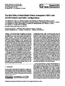
Fig. 1. Stream function of the Atlantic meridional overturning circulation for the reference state and the four targets. Figure 1
model years from the state of rest with the external forcings based on the protocol of the Coordinated Ocean-ice Reference Experiments (COREs) project (Griffies et al., 2009). We used a tracer acceleration method with a time step of 1 day for the tracer equations and 20 min for the momentum equations. The maximum of the Atlantic meridional overturning stream function of 18.3 Sv was taken as a measure of the AMOC strength in the reference state. The reference configuration was modified considerably to generate Targets 1 and 2. In both runs the prescribed atmospheric fields were replaced by fields from a coupled atmospheric energy–moisture balance model (Ashkenazy et al., 2013). These simulations corresponded to very different climates, mostly as a consequence of the dynamic interaction of the ocean with the atmosphere, although some of the internal ocean model parameters were also modified (Table 2). After another spin-up of 2000 years we added freshwater to the North Atlantic Ocean uniformly between 20◦ N and 50◦ N at a rate of 0.28 Sv for an additional 1000-year run. We calculated the Atlantic meridional overturning stream function and took the maximum of 11.4 Sv as an indication of a reduced AMOC strength for Target 1 as compared to the reference state. The unmodified run with an increased rate of 23.7 Sv became Target 2. Targets 3 and 4 were generated by increasing or reducing internal physical parameters that determine the lateral eddy viscosity for additional 200-year runs from the reference. These parameters for harmonic and bi-harmonic viscosity (A∗h , A∗4 ) were not used as standard control variables in our experiments. Increasing the eddy viscosity led to a smaller overturning rate of 12.5 Sv (Target 3) as compared to the reference state, decreasing to a larger overturning rate of 22.9 Sv (Target 4). Targets 1 and 3 had similarly weak AMOC strengths and Targets 2 and 4 similarly stronger AMOC strengths, but Geosci. Model Dev., 7, 419–432, 2014
422
T. Kurahashi-Nakamura et al.: Ocean reconstruction from sparse data
Table 1. Summary of experiment settings and results. Used data are specified as follows. ST: surface temperature from MARGO data locations, DT: Deep temperature from MARGO data locations, AST: surface temperature from all other grid cells, SS: surface salinity from MARGO data locations, DS: deep salinity from MARGO data locations, and ASS: surface salinity from all other grid cells. Maximum values of the AMOC stream function are shown in Sv (1 Sv = 106 m3 s−1 ). Reconstructed AMOC strength that is closer to the target than half of the difference between the starting point (reference state) and target is shown in italics. The rightmost column shows the mean cost (i.e., the value of objective function divided by the number of model-data comparisons). The unit of data error σ is K for temperature and psu for salinity. Used data Experiment
ST
DT
AST
SS
DS
ASS
Maximum of AMOC stream function (Sv)
Data errors
Reference state
Mean cost (× 10−1 )
18.3
Target 1 E1-1 E1-2 E1-3 E1-4 E1-5 E1-6 E1-7 E1-8
x x x x x x x x
Target 2 E2-1 E2-2 E2-3 E2-4 E2-5 E2-6 E2-7 E2-8
x x x x x x x x
Target 3 E3-1 E3-2 E3-3
x x x
Target 4 E4-1 E4-2 E4-3
x x x
x x x x x x
x x
x x
x
x
x
x
x
x
x x x x x x
x x
x x
x
x
x
x
x
x
Targets 1 and 2 were much colder than both the reference and Targets 3 and 4 (Table 2). The temperature and salinity distributions of each target were sampled and averaged over the last 10 years of the simulations. Surface data (SST and SSS) were taken from the top grid nodes, deep-ocean data from the bottom grid nodes. Normally distributed noise with a standard deviation of the prior errors was added as a random error to obtain the pseudo-data. Note that large uncertainties were associated with proxy data so that the prior errors (see below) could be large. This led to the realistic situation that the proxy data could be strongly biased after adding large noise contributions on the order of, for example, 1 ◦ C. Starting from the reference run, the ocean model was fitted to the pseudo-proxy data by minimizing the following
Geosci. Model Dev., 7, 419–432, 2014
11.4 39.1 19.5 31.4 13.8 20.3 21.5 14.2 16.1
0.74 6.4 4.8 9.6 5.4 9.7 35 74
23.7 30.5 18.9 43.8 37.4 18.8 24.9 14.6 29.5
0.36 6.3 4.1 9.7 5.1 8.5 36 82
MARGO σ = 0.1 MARGO
12.5 13.7 14.3 14.9
2.9 44 9.2
MARGO σ = 0.1 MARGO
22.9 30.2 20.2 21.8
3.0 18 9.4
MARGO MARGO/σ MARGO MARGO/σ MARGO/σ MARGO/σ σ = 0.1 σ = 0.1 MARGO MARGO/σ MARGO MARGO/σ MARGO/σ MARGO/σ σ = 0.1 σ = 0.1
= 2.0 = 2.0 = 2.0 = 2.0
= 2.0 = 2.0 = 2.0 = 2.0
objective function J : J = (Tmodel − Ttarget )T Wt (Tmodel − Ttarget ) + (Smodel − Starget )T Ws (Smodel − Starget ) ,
(1)
where Tmodel and Smodel were the average over the last 10 years of a 20-year integration (for each iteration) of temperature and salinity, Ttarget and Starget were pseudo-proxy data based on the artificial targets, Wt and Ws were weight matrices that were the inverse of the error covariance matrices. All errors were assumed to be uncorrelated, so that the inverse error covariances reduced to scalar weights. To reconstruct the targets, we used the following control variables: the radiative and wind forcing at the sea surface, the air temperature, the humidity above the sea surface, the precipitation, and the initial temperature and salinity. Every control www.geosci-model-dev.net/7/419/2014/
T. Kurahashi-Nakamura et al.: Ocean reconstruction from sparse data
423
Table 2. Summary of model configurations for the reference state and the targets. Parameters
Reference
Normalized lateral eddy viscosity A∗h (non-dim.) Normalized biharmonic viscosity A∗4 (non-dim.) Vertical eddy viscosity (r 2 /s)
1.2 × 10⁻²
Vertical diffusion coefficient (m2 /s) Parameterization scheme for vertical mixing
Parameterization scheme for geostrophic eddies
Mean absolute deviation of sea-surface temperature (SST) from the reference Root mean square of SST difference from the reference
Target 2
Target 3
Target 4
0 3.0 × 10⁻¹ 1.0 × 10⁻³ 3.0 × 10⁻⁵ Nonlocal K-profile parameterization (KPP) GM with variable eddy coefficientsb 2.9 K
1.0 × 10⁻³ 3.0 × 10⁻⁵ implicit vertical diffusion
5.0 × 10⁻³ 5.0 × 10⁻² 1.0 × 10⁻³ 3.0 × 10⁻⁵ implicit vertical diffusion
Redi/GM parameterizationa –
0 3.0 × 10⁻¹ 1.0 × 10⁻³ 3.0 × 10⁻⁵ Nonlocal K-profile parameterization (KPP) GM with variable eddy coefficientsb 2.9 K
1.5 × 10⁻²
Redi/GM parameterizationa 0.14 K
Redi/GM parameterizationa 0.16 K
–
3.5 K
3.4 K
0.3 K
0.3 K
1.2 × 10⁻¹ 1.0 × 10⁻³ 3.0 × 10⁻⁵ implicit vertical diffusion
Target 1
1.5 × 10⁻¹
a Redi (1982); Gent and McWilliams (1990); Gent et al. (1995). b Visbeck et al. (1997).
variable was normalized according to the characteristic scale of each variable, and was smoothed with a 9-point smoothing scheme. A quasi-Newton algorithm (Gilbert and Lemaréchal, 1989) was used to iteratively find optimized control variables that minimized J . The essential gradient information was provided by the adjoint model. To explore the potential information content of the MARGO data set, the first experiments with Targets 1 and 2 only used the model SST sampled at the MARGO core locations as pseudo-proxy data (Table 1). For these data, we used prior data errors derived from the uncertainty estimated for each individual data point by the MARGO project (MARGO Project Members, 2009). MARGO uncertainty estimates are conservative and meant to give an upper bound. If a model grid cell contained more than one data point, the weighted average of all data points was used. Then we successively added hypothetical data sets to improve the data coverage and to assess its effect on the state estimates. We assigned prior errors to the hypothetical data points as specified in Table 1. We used the same prior errors for temperature and salinity. 3
Results
Table 1 summarizes the experiments. A simple measure of the quality of the model fit after the optimization is based on the principles of a χ -squared test. The scaled contributions to the cost function are assumed to be independent Gaussian variables with an expectation value of one, so that the expectation value of a well-balanced problem is the number of model–data comparisons. Therefore, the mean cost (i.e., cost function divided by the number of model-data comparisons) is of the order of one or less (Wunsch, 1996, 2006). In all of our experiments with MARGO data errors the mean www.geosci-model-dev.net/7/419/2014/
cost function value was less than one, so that we called the model-fitting itself successful (rightmost column of Table 1). For the other experiments with the much smaller data errors of σ = 0.1, the values were larger than one. This implied that the fit was not successful and the hypothesis that the model was consistent with the data within prior errors had to be rejected. Nevertheless, the stricter requirements for the fit meant that the model was generally closer to observations and thus better constrained than with the larger errors (also see below). Those experiments for which the AMOC strength was adjusted by the least-squares fit to be closer to the target than half of the difference between the starting point (reference state) and target were marked as successful in reconstructing the overturning. These were experiments E1-4 and E1-7 for Target 1 and E2-6 for Target 2. For Targets 3 and 4 all experiments except for E4-1 and E4-2 were successful by this measure. The other experiments had either far too large an overturning rate or the overturning rate was not affected by the constraining observations. For the two targets with a much colder climate (Targets 1 and 2) the results were incoherent. Surface data of temperature (E1-1 and E2-1) and salinity (E1-3 and E2-3) alone did not appear to be sufficient to constrain the overturning rate. Instead, assimilating these data led to much too strong an overturning in all cases, even for Target 1 where the sampled surface data corresponded to a weaker overturning rate. Temperature data alone at the surface and near the bottom were also without effect. In these runs (E1-2 and E2-2), the overturning rate hardly changed relative to the initial guess. Temperature and salinity data near the bottom were required to bring the overturning rate down to the target value in E14, or to enhance it in E2-4 (but here they led to too strong an overturning). A large effect of salinity data on the overturning
Geosci. Model Dev., 7, 419–432, 2014
424
T. Kurahashi-Nakamura et al.: Ocean reconstruction from sparse data E1-1
E1-3
E1-5
E1-6
E1-2
E1-4
E1-7
E1-8
50 N
30 N
50 N
30 N
60 w
30 w
60 w
30 w
-5
60 w
0 [K]
30 w
60 w
30 w
5
Fig. 2. Anomalies of temperature at the depth of 2000 m in E1-1–E1-8 compared to Target 1.
rate was clearly seen in the comparison between E1-2 and E1-4, and between E2-2 and E2-4. In runs E1-5, E1-6, E2-5, and E2-6 we assumed that the data were available at all surface grid points. Even the complete data coverage of SST was insufficient to reconstruct the AMOC properly for both targets. This may not come as a surprise, because even a current monitoring for modern AMOC (e.g., Srokosz et al., 2012) needs more elaborate information including sea-surface height data to precisely constrain AMOC behavior. With both temperature and salinity data at all surface grid points, one experiment (E2-6) was successful in reproducing the larger overturning rate of Target 2. If we were able to increase the data accuracy, for example, by increasing the number of observations within a grid cell or by inventing new proxies that would yield a more accurate reconstruction of temperature and salinity, we could hope to improve the state estimates. In experiment E1-7 accurate temperature data alone was sufficient for a good agreement of the overturning rate to Target 1. The same configuration led to an adjustment with the wrong sign in E2-7. Accurate temperature and salinity data marginally improved the agreement with the targets’ overturning rates compared to other experiments, but not sufficiently to be called successful. The second set of targets (Targets 3 and 4) was created with the same atmospheric forcing as for the reference state, but internal model parameters were modified to mimic inherent model biases. Identical twin experiments, in which the control parameters consisted of just these modified viscosity parameters, confirmed that the system was able to completely recover the original parameters. These experiments only represent a (successful) zero-order test showing that the system works with a perfect model. For the standard control variables (initial conditions and atmospheric forcing fields, see above), the first pair of experiments for Target 3 and 4 (E3-1 and E4-1) showed that, provided the targets were close enough to the reference (i.e., the first guess) with regard to the temperature (Table 1), the same data distribution Geosci. Model Dev., 7, 419–432, 2014
and errors as those for E1-1 and E2-1 were sufficient to guide the AMOC strength to the right direction, even if the target strengths were much different from that of the reference Figure 2 much smaller data prior errors (E4-2), the esstate. With timated AMOC strength for Target 4 was better estimated compared to E4-1, although E3-2 was slightly worse than E3-1. For the last two experiments (E3-3 and E4-3) we reduced the control space to the initial conditions, as well as the surface wind stress and the incoming shortwave and longwave radiative fluxes (i.e., reducing the number of control variables from nine to six, which made the model less flexible, see also Sect. 4.2). Even without the air temperature, the humidity, and the precipitation as control variables, the AMOC strength were successfully estimated.
4 4.1
Discussion Analysis of the results for Targets 1 and 2
The experiments for Targets 1 and 2 showed that more data or data with smaller errors did not necessarily lead to a better AMOC reconstruction. However, the seemingly incoherent tendency toward different solutions can be explained as follows. In all experiments for both Targets 1 and 2, very strong vertical mixing occurred in the high-latitude North Atlantic at the beginning of each of the optimization runs, because the model adjusted to the much colder target SST, implying denser surface water. For the experiments for Target 1 the further development of the solution depended on whether the ocean could recover from the “initial shock" of strong mixing or not. With no or insufficient contribution of the deep-ocean data (E1-1, E13, E1-5, and E1-6) the lighter (i.e., warmer) deep water of the reference ocean tended to remain (Fig. 2), so that mixing continued. Note that temperature and salinity data of the deep www.geosci-model-dev.net/7/419/2014/
T. Kurahashi-Nakamura et al.: Ocean reconstruction from sparse data
425
E2-1
E2-2
E2-5
E2-7
E2-3
E2-4
E2-6
E2-8
50 N
30 N
50 N
30 N
60 w
30 w
60 w
30 w
-3
60 w
0 [ psu ]
30 w
60 w
30 w
3
Fig. 3. Anomalies of the sea-surface salinity in E2-1–E2-8 compared to Target 2.
ocean were also used in E1-5 and E1-6, but their contribution was very small, because the weight of the deep-ocean data decreased relative to the surface-ocean data in proportion of the number of data points. Among the other experiments (E12, E1-4, E1-7, and E1-8) only E1-2 failed completely, while the other three were able to predict the direction of change of the AMOC strength because of the deep-ocean data. Comparing it with E1-7 that had the same data locations, E1-2 still had a larger warm anomaly in the deep North Atlantic that was poorly constrained by data with larger errors. The warm water supported the relatively strong mixing. For the experiments for Target 2, the warm deep water of the reference state also helped to maintain the strong mixing. Without any salinity constraints, however, the surface water became too light (too fresh), because there was less evaporation with the colder SST and freshwater was also advected from the south (Fig. 3). This effect caused the overly weak AMOC in E2-2, E2-5, and E2-7. Although the same mechanism worked to some extent also in E2-1, strong warm anomalies in the deep North Atlantic remained due to the lack of deep-ocean data, which caused continuing strong convection similar to the case of Target 1. By analogy with E1-5 and E1-6, and because of the very small contribution of the deep-ocean data, one might expect that E2-5 would have a similar problem as E2-1, but the SST was adjusted in a much larger area in E2-5 than in E2-1 so that more fresh surface water was created. The AMOC was weaker because the excess of freshwater outweighed the effects of low abyssal densities in the absence of deep-ocean data. We further examined the mixed layer depth (MLD) and the location of deep convection in the high-latitude North Atlantic in some of the experiments (Figs. 4 and 6). Different AMOC strength during the LGM have been suggested to be associated with a shift in the location of deep convection (e.g., Rahmstorf, 1994; Ganopolski and Rahmstorf, 2001; Oka et al., 2012). The reference state had its deepest convection site in the Labrador Sea, while Target 1 had one near www.geosci-model-dev.net/7/419/2014/
Iceland. Although all four reconstructions shown in Fig. 4 shifted the convection sites roughly to the right place, the Figure 3 not be recovered. In the experiments with a good depth could AMOC strength estimate for Target 1 (e.g., E1-4), the MLD shoaled from the reference state as for Target 1 (Fig. 4a). Experiments that failed in reconstructing the weaker AMOC strength had a deeper MLD (E1-1, 2, 6 in Fig. 4a). This was consistent with an overly strong AMOC in the reconstructions; especially for the experiments with a very strong AMOC strength (E1-1). As before, the MLD of the state estimates was related to the temperature in the deep ocean. While the temperature field at 1000 m depth for E1-4 was similar to the target temperature (Fig. 4b), the deep ocean was too warm in the other three experiments, especially in E1-1 and E1-6. Similarly, the deep-ocean salinity at 1000 m depth was too high in the other experiments as compared to E1-4 (Fig. 4d). On the other hand, the temperature field (Fig. 4c) and the salinity fields (Fig. 4e) at 3000 m clearly distinguished E1-4 and E1-2 from E1-1 and E1-6. This was related by the vertical distribution of the data in the North Atlantic Ocean (Fig. 5). Because a relatively large number of deep-ocean data were located around at 3000 m depth, the reconstructions at those depths were greatly affected by whether the deep-ocean data were used or not for the state estimation. The availability of data also affected E1-7 and E1-8, because the difference between them was caused by different temperature and salinity reconstructions in the ocean interior at depths shallower than 500 m, where there were almost no data points. This result emphasized the importance of data at those depths, even though the convection of the target could be roughly reconstructed from surface information. It was consistent with the sensitiveness of AMOC to the temperature at those depths (Heimbach et al., 2011; Heslop and Paul, 2012). Heslop and Paul (2012) showed that the AMOC strength was more sensitive to ocean temperature at depths shallower than 1000 m compared to the deeper ocean. Geosci. Model Dev., 7, 419–432, 2014
426
T. Kurahashi-Nakamura et al.: Ocean reconstruction from sparse data Target 1 - Ref.
E1-4 - Ref.
E1-2 - Ref.
E1-1 - Ref.
E1-6 - Ref.
2000 [m]
50 N
(a)
0
30 N -2000 5 [K]
50 N
(b)
0
30 N -5 3 [K]
50 N
(c)
0
30 N -3 1 [psu]
50 N
(d)
0
30 N -1 0.2 [psu]
50 N
(e)
0
30 N
60 w
30 w
60 w
30 w
60 w
30 w
60 w
30 w
60 w
30 w
-0.2
Figure 4
Fig. 4. Anomalies in Target 1, E1-4, E1-2, E1-1, and E1-6 compared to the reference state: the maximum monthly averaged mixed layer depth (a), the temperature at the depth of 1000 m (b) and 3000 m (c), and the salinity at the depth of 1000 m (d) and 3000 m (e). In (a), the deepest convection site is shown as a red ellipse for the reference state and as a blue ellipse for Target 1 and each experiment.
Geosci. Model Dev., 7, 419–432, 2014
0
Depth [m]
Huybers et al. (2007) also demonstrated that data in the ocean interior is important for reliable circulation estimates. Along with these studies our results explicitly suggested that there are shortcomings in the vertical distribution of MARGO data (Fig. 5). For Target 2, experiments E2-6, which successfully reproduced the stronger AMOC, and E2-8 showed a similar MLD anomaly with respect to the target (Fig. 6a; albeit the positive anomalies in E2-8 were too large, corresponding to the overly high rate of overturning in this experiment). However, in E2-7, the positive MLD anomaly was smaller, causing a much weaker AMOC than in the target. As discussed above, the sea-surface salinity (SSS) was very different for E2-7 compared to E2-6 and E2-8 (Fig. 6b). The low SSS of E27 caused low density of surface water which stabilized the water column and reduced deep mixing. The principal location of deep convection of Target 2 (to the southeast of Iceland) was successfully predicted in every experiment (i.e., irrespective of the AMOC strength). As for Target 1, although the shifts in the location of deep convection were also observed in all experiments, only some experiments succeeded in predicting exactly the locations of the target. However, those experiments did not necessarily reconstruct the proper AMOC strength. These results suggested that predicting the MLD was not equivalent to predicting the location of deep convection. We note that the representation
0
-500
-500
-1000
-1000
-1500
-1500
-2000
-2000
-2500
-2500
-3000
-3000
-3500
-3500
-4000
-4000
-4500
-4500
-5000
0
5
10
15 20 40 60 80
-5000
The number of grid cells with data
Fig. 5. Vertical distribution of theFigure data in5the North Atlantic Ocean. The number of grid cells that contain any data in the domain illustrated in Fig. 4 is shown as a function of depth.
www.geosci-model-dev.net/7/419/2014/
T. Kurahashi-Nakamura et al.: Ocean reconstruction from sparse data Target 2 - Ref.
E2-6 - Ref.
427
E2-8 - Ref.
E2-7 - Ref.
3000
50 N
(a)
0 [m]
30 N -3000 -3
50 N
(b)
0 [ psu ]
30 N
60 w
30 w
60 w
30 w
60 w
30 w
60 w
3
30 w
Fig. 6. Anomalies in Target 2, E2-6, E2-8, and E2-7 compared to the reference state: the maximum monthly averaged mixed layer depth (a), and the sea-surface salinity (b). In (a), the deepest convection site is shown as a red ellipse for the reference state and as a blue ellipse for Target 2 and each experiment.
Target 3 - Ref.
The pseudo data with MARGO errors - Ref.
E3-1 - Ref.
E3-2 - Ref.
E3-3 - Ref.
E4-2 - Ref.
E4-3 - Ref.
Figure 6
50 N
(a) 30 N
Target 4 - Ref.
The pseudo data with MARGO errors - Ref.
E4-1 - Ref.
50 N
(b) 30 N
60 w
30 w
60 w
30 w
60 w
-4
30 w
0 [K]
60 w
30 w
60 w
30 w
4
Fig. 7. Anomalies of the sea-surface temperature compared to the reference state in Target 3, the pseudo-data with the MARGO errors, E3-1, E3-2, and E3-3 (a), and Target 4, the pseudo-data, E4-1, E4-2, and E4-3 (b).
Figure 7
of the MLD may be affected by the low vertical resolution of the model, but the targets and the model were sufficiently similar (in fact the vertical resolution is the same) so that the resolution did not affect our results. When fitting to real proxy data, however, vertical resolution may become an issue when data are mapped to model levels or MLD is estimated. On the other hand, we emphasize that the coarse resolution has the great advantage of low computational cost and relatively few degrees of freedom (especially given the apparently scarce data). The shift of deep convection sites could be one factor that complicated the reconstruction, because very different sinking locations represent non-linear “jumps" between the targets and the reference. Another difficulty for reconstruction was that Targets 1 and 2 used entirely different parameterisations of mixing than the assimilation model (Table 2), which meant that large model errors needed to be overcome. Large model errors and non-linearities are anticipated when attempting to reconstruct the real LGM ocean, hence we deliberately chose such a diverse target for our tests. Other sources
www.geosci-model-dev.net/7/419/2014/
of non-linearity may be found in the sea-ice model. However, the reconstructed sea-ice distribution (not shown) was getting better with more (or better) data even if the AMOC was not. This implied that the sea ice can be reconstructed more straightforwardly than the AMOC and can be interpreted more easily. We did not find a coherent surface fingerprint of the AMOC (e.g., Zhang, 2008) in our simulations. In comparison to Zhang (2008), the large difference regarding the timescale of phenomena need to be taken into account. Zhang (2008) dealt with decadal variability, while our focus was on a quasisteady state including the deep ocean. Therefore, information from the deep ocean was required to constrain the model. Otherwise, a very long time period of assimilation would be required so that the information at the surface could penetrate the entire ocean. 4.2
Outlook for reconstructions with a better first guess
The experiments for Targets 1 and 2 demonstrated that the targets were not consistently reconstructed, even when we Geosci. Model Dev., 7, 419–432, 2014
428
T. Kurahashi-Nakamura et al.: Ocean reconstruction from sparse data (a)
(b)
(c)
Target 3 - Ref.
E3-3 - Ref.
Target 3 - Ref.
E3-3 - Ref.
Target 3 - Ref.
E3-3 - Ref.
Target 4 - Ref.
E4-3 - Ref.
Target 4 - Ref.
E4-3 - Ref.
Target 4 - Ref.
E4-3 - Ref.
50 N
30 N
50 N
30 N 60 w
30 w
-10-5
60 w
0 [kg/m2/s]
30 w
10-5
60 w
60 w
30 w
-0.5
30 w
0.5
0 [K]
60 w
30 w
-0.7
60 w
0 [ psu ]
30 w
0.7
Fig. 8. Anomalies in Target 3, E3-3, Target 4, and E4-3 compared to the reference state: the freshwater flux (a), the sea-surface temperature Figure 8 (b), and the sea-surface salinity (c).
assumed very optimistic conditions for data quality and quantity, and in spite of the fact that the atmospheric state that was responsible for the differences was part of the control vector and was adjusted in the optimization process. The results suggested that it was difficult with the available data to guide the model properly towards targets that were very different from the first guess. Providing prior knowledge, that is, a better first guess may alleviate the problem as illustrated in the following. We remind the reader that for Targets 3 and 4 internal friction parameters were modified that were not part of the control vector. This choice introduced a model bias that could not be adjusted by the assimilation in the “correct” way, a situation that is definitely encountered in every state estimation exercise. In all three pairs of experiments for Target 3 and 4, the AMOC corrections relative to the first guess had the correct sign. However, there were large differences between the temperature fields of those experiments (Fig. 7). The SST fields of E3-1 and E4-1 were very different from those of their respective target fields (third column in Fig. 7), because the noisy pseudo-data to which the model adjusted was also very different from the original targets due to the large associated uncertainty (second column of Fig. 7). The experiments with very small data errors and accordingly reduced noise in the data (E3-2 and E4-2) did not have this problem and hence the agreement between model and target was much better (fourth column in Fig. 7). The experiments with fewer control variables (E3-3 and E4-3, fifth column in Fig. 7) avoided the overfitting to data of poor quality (i.e., data with a low signal-to-noise ratio) by using a less flexible model that restricted the departure from the first guess. This amounted to providing even more prior knowledge, as we assumed implicitly that air temperature, humidity and precipitation were well known. The good NADW reconstruction in E3-3 and E4-3 was connected to the modified freshwater flux in the high-latitude North Atlantic (Fig. 8a). Note that the surface freshwater flux was not part of the control vector in this case. Instead, changes in the surface freshwater flux were caused Geosci. Model Dev., 7, 419–432, 2014
by adjustments of the incoming radiative fluxes that led to changes in temperature and thus to changes in evaporation. For E3-3, this positive freshwater flux anomaly, consistent with the difference in freshwater flux between the target and the reference state, stabilized the water column and inhibited NADW formation. In contrast, a negative freshwater anomaly destabilized the water column and led to increased NADW formation in E4-3. The difference between the target and the reference state was also generally negative. Similar patterns of the SST and freshwater flux anomalies (Fig. 8b) show that the evaporation rate was strongly controlled by the SST. Consequently, adjusting the SST in the high-latitude North Atlantic to the target values led to a successful reconstruction of the AMOC. By way of this freshwater flux anomaly, the SST adjustment roughly reproduced the sea-surface salinity (SSS) without using SSS as a constraint (Fig. 8c), because the SSS anomalies in the targets were also, in part, caused by the change in evaporation due to SST changes.
5
Conclusions
Can we use sparse paleoceanographic proxy data to reconstruct the strength of the AMOC during the LGM, using the MITgcm? Our answer is twofold: (1) with a sufficiently good first guess, one can indeed reconstruct the strength of the AMOC from sparse sea-surface temperature data such as the existing MARGO data set. (2) Otherwise, however, it is important to obtain data from the deep-ocean and salinity data. Although naturally small data uncertainties would help, sampling data at adequate locations seems to be a crucial factor for proper estimation of the AMOC change. Although a good first guess with a reasonable representation of past hydrographic conditions would be very helpful, finding such a first guess is essentially part of the state estimation that we are aiming for. A further problem to be addressed is overfitting the model to data with a poor signal-tonoise ratio. Both issues could be addressed by adding either www.geosci-model-dev.net/7/419/2014/
T. Kurahashi-Nakamura et al.: Ocean reconstruction from sparse data more data (once available) or prior knowledge. One way of adding prior knowledge would be re-considering the control parameter space and adding more model physics. In particular, the surface fluxes could be more physically constrained by coupling the ocean model to an atmospheric model, for example, an energy–moisture balance model (e.g., Ashkenazy et al., 2013). An advantage of this would be that one would be able to remove a systematic bias (e.g., globally lower temperature) before the spatial patterns of smaller scale are adjusted according to the local paleoceanographic reconstruction based, for example, on MARGO. It should be noted that Targets 1 and 2 were more difficult to reconstruct than 3 and 4 because they had not only different spatial patterns (of temperature and salinity) but also a much different global mean temperature. After we remove the systematic bias of mean temperature for LGM as much as possible, the adjustment of local patterns would become easier. Using such a coupled model could enable more control over the global SST by changing, for example, the CO2 content of the atmosphere, the planetary albedo or the atmospheric heat transport efficiency (Paul and Losch, 2012). Note that the CO2 content and the ice-sheet distribution during the LGM are comparatively well known. At the same time, one could decrease the degrees of freedom of the model by reducing the control variables. Alternatively, one could imagine using the results of LGM simulations with different coupled GCMs (e.g., the PMIP project (Otto-Bliesner et al., 2007)) to improve the initial guess. A more direct but less physical way to add prior knowledge is to enforce smoothness through a Laplacian of some physical quantity (e.g., surface temperature) or to penalize deviations from the first guess; this, however, is only possible at the cost of introducing more biases. From the viewpoint of paleo-ocean data, proxies for water masses (δ 13 C), circulation rates (radiocarbon, 231 Pa/230 Th ratios) and density (δ 18 O, possibly in combination with a temperature proxy such as Mg/Ca) may also provide useful additional constraints. This point, as well as the importance of smaller data uncertainty, is also suggested by Huybers et al. (2007). However, it should be noted that a simplified model such as the one used by Huybers et al. (2007) involves uncertainty due to a subjectively assumed level of no motion (see also Burke et al., 2011). Besides, the model domain of Huybers et al. (2007) excludes depths shallower than 1 km. Therefore, they do not discuss the effectiveness of surface data that are the main components of the currently available data archive, such as the MARGO data. Our results showed how important surface data are for predicting the convection. The integration period in the state estimates (20 years) was chosen for purely economical reasons, and our simulations were not long enough to guarantee stable steadystate solutions. Cost function terms that penalize inter-annual variations could be used to enforce a steady state. Alternatively, longer integration periods for each iteration would be required. Paleo-data from regions where Antarctic Bottom Water is formed may become more important on longer www.geosci-model-dev.net/7/419/2014/
429
timescales, because the relative densities of the North Atlantic and Southern Ocean source waters are expected to play a larger role for the meridional overturning circulation in the steady-state problem (e.g., Paul and Schäfer-Neth, 2003; Weber et al., 2007). However, in our experiments the adjustment of the AMOC was very fast; it typically occurred in the first 10 years of a 20-year experiment. This was also plausible from the timescale of sensitivity propagation of the AMOC, shown by Heimbach et al. (2011). Therefore, the time interval was assumed to be sufficient for estimating the change of the AMOC strength.
Acknowledgements. This research was funded by the DFGResearch Center/Center of Excellence MARUM – “The Ocean in the Earth System”. We thank two anonymous reviewers for their insightful review and helpful comments. The adjoint model was generated with TAF (Giering and Kaminski, 1998). Edited by: J. Annan
References Adcroft, A., Campin, J.-M., Hill, C., and Marshall, J.: Implementation of an Atmosphere Ocean General Circulation Model on the Expanded Spherical Cube, Mon. Weather Rev., 132, 2845, doi:10.1175/MWR2823.1, 2004. Adkins, J. F., McIntyre, K., and Schrag, D. P.: The Salinity, Temperature, and δ 18 O of the Glacial Deep Ocean, Science, 298, 1769– 1773, doi:10.1126/science.1076252, 2002. Archer, D.: Modeling the calcite Lysocline, J. Geophys. Res., 96, 17037, doi:10.1029/91JC01812, 1991. Archer, D., Winguth, A., Lea, D., and Mahowald, N.: What caused the glacial/interglacial atmospheric pCO2 cycles?, Rev. Geophys., 38, 159–189, doi:10.1029/1999RG000066, 2000. Ashkenazy, Y., Losch, M., Gildor, H., Mirzayof, D., and Tziperman, E.: Multiple sea-ice states and abrupt MOC transitions in a general circulation ocean model, Clim. Dyanm., 40, 1803–1817, doi:10.1007/s00382-012-1546-2, 2013. Burke, A., Marchal, O., Bradtmiller, L. I., McManus, J. F., and François, R.: Application of an inverse method to interpret 231 Pa/230 Th observations from marine sediments, Paleoceanography, 26, PA1212, doi:10.1029/2010PA002022, 2011. Clark, P. U., Marshall, S. J., Clarke, G. K. C., Hostetler, S. W., Licciardi, J. M., and Teller, J. T.: Freshwater Forcing of Abrupt Climate Change During the Last Glaciation, Science, 293, 283–287, doi:10.1126/science.1062517, 2001. Curry, W. B. and Oppo, D. W.: Glacial water mass geometry and the distribution of δ 13 C of 6CO2 in the western Atlantic Ocean, Paleoceanography, 20, PA1017, doi:10.1029/2004PA001021, 2005. Dail, H. J.: Atlantic Ocean Circulation at the Last Glacial Maximum: Inferences from Data and Models, Ph.D. thesis, Massachusetts Institute of Technology, Massachusetts and the Woods Hole Oceanographic Institution, Massachusetts, 2012. Epica Community Members, Barbante, C., Barnola, J.-M., Becagli, S., Beer, J., Bigler, M., Boutron, C., Blunier, T., Castellano, E., Cattani, O., Chappellaz, J., Dahl-Jensen, D., Debret, M., Delmonte, B., Dick, D., Falourd, S., Faria, S., Federer, U., Fischer,
Geosci. Model Dev., 7, 419–432, 2014
430
T. Kurahashi-Nakamura et al.: Ocean reconstruction from sparse data
H., Freitag, J., Frenzel, A., Fritzsche, D., Fundel, F., Gabrielli, P., Gaspari, V., Gersonde, R., Graf, W., Grigoriev, D., Hamann, I., Hansson, M., Hoffmann, G., Hutterli, M. A., Huybrechts, P., Isaksson, E., Johnsen, S., Jouzel, J., Kaczmarska, M., Karlin, T., Kaufmann, P., Kipfstuhl, S., Kohno, M., Lambert, F., Lambrecht, A., Lambrecht, A., Landais, A., Lawer, G., Leuenberger, M., Littot, G., Loulergue, L., Lüthi, D., Maggi, V., Marino, F., MassonDelmotte, V., Meyer, H., Miller, H., Mulvaney, R., Narcisi, B., Oerlemans, J., Oerter, H., Parrenin, F., Petit, J.-R., Raisbeck, G., Raynaud, D., Röthlisberger, R., Ruth, U., Rybak, O., Severi, M., Schmitt, J., Schwander, J., Siegenthaler, U., Siggaard-Andersen, M.-L., Spahni, R., Steffensen, J. P., Stenni, B., Stocker, T. F., Tison, J.-L., Traversi, R., Udisti, R., Valero-Delgado, F., van den Broeke, M. R., van de Wal, R. S. W., Wagenbach, D., Wegner, A., Weiler, K., Wilhelms, F., Winther, J.-G., and Wolff, E.: One-to-one coupling of glacial climate variability in Greenland and Antarctica, Nature, 444, 195–198, doi:10.1038/nature05301, 2006. Errico, R. M.: What Is an Adjoint Model?, B. Am. Meteorol. Soc., 78, 2577–2591, doi:10.1175/15200477(1997)0782.0.CO;2, 1997. Fischer, G. and Wefer, G.: Use of Proxies in Paleoceanography: Examples from the South Atlantic, Springer Berlin Heidelberg, available at: http://books.google.de/books?id=e8lIokyIG7gC, 1999. Ganopolski, A. and Rahmstorf, S.: Rapid changes of glacial climate simulated in a coupled climate model, Nature, 409, 153– 158, doi:10.1038/35051500, 2001. Gebbie, G. and Huybers, P.: Meridional circulation during the Last Glacial Maximum explored through a combination of South Atlantic δ 18 O observations and a geostrophic inverse model, Geochem. Geophy. Geosys., 7, Q11N07, doi:10.1029/2006GC001383, 2006. Gent, P. R. and McWilliams, J. C.: Isopycnal Mixing in Ocean Circulation Models, J. Phys. Oceanogr., 20, 150–160, doi:10.1175/1520-0485(1990)0202.0.CO;2, 1990. Gent, P. R., Willebrand, J., McDougall, T. J., and McWilliams, J. C.: Parameterizing Eddy-Induced Tracer Transports in Ocean Circulation Models, J. Phys. Oceanogr., 25, 463–474, doi:10.1175/1520-0485(1995)0252.0.CO;2, 1995. Giering, R. and Kaminski, T.: Recipes for adjoint code construction, ACM Trans. Math. Softw., 24, 437–474, doi:10.1145/293686.293695, 1998. Gilbert, J. C. and Lemaréchal, C.: Some numerical experiments with variable-storage quasi-Newton algorithms, Math. Prog., 45, 407–435, doi:10.1007/BF01589113, 1989. Gildor, H. and Tziperman, E.: Physical mechanisms behind biogeochemical glacial-interglacial CO 2 variations, Geophys. Res. Lett., 28, 2421–2424, doi:10.1029/2000GL012571, 2001. Griffies, S. M., Biastoch, A., Böning, C., Bryan, F., Danabasoglu, G., Chassignet, E. P., England, M. H., Gerdes, R., Haak, H., Hallberg, R. W., Hazeleger, W., Jungclaus, J., Large, W. G., Madec, G., Pirani, A., Samuels, B. L., Scheinert, M., Gupta, A. S., Severijns, C. A., Simmons, H. L., Treguier, A. M., Winton, M., Yeager, S., and Yin, J.: Coordinated Ocean-ice Reference Experiments (COREs), Ocean Model., 26, 1–46, doi:10.1016/j.ocemod.2008.08.007, 2009.
Geosci. Model Dev., 7, 419–432, 2014
Heimbach, P., Hill, C., and Giering, R.: An efficient exact adjoint of the parallel MIT general circulation model, generated via automatic differentiation, Future Gener. Comput. Sy., 21, 1356–1371, doi:10.1016/j.future.2004.11.010, 2005. Heimbach, P., Wunsch, C., Ponte, R. M., Forget, G., Hill, C., and Utke, J.: Timescales and regions of the sensitivity of Atlantic meridional volume and heat transport: Toward observing system design, Deep Sea Res.-Pt. II, 58, 1858–1879, doi:10.1016/j.dsr2.2010.10.065, 2011. Heslop, D. and Paul, A.: Fingerprinting of the Atlantic meridional overturning circulation in climate models to aid in the design of proxy investigations, Clim. Dynam., 38, 1047–1064, doi:10.1007/s00382-011-1042-0, 2012. Huybers, P., Gebbie, G., and Marchal, O.: Can Paleoceanographic Tracers Constrain Meridional Circulation Rates?, J. Phys. Oceanogr., 37, 394, doi:10.1175/JPO3018.1, 2007. Keigwin, L. D. and Lehman, S. J.: Deep circulation change linked to HEINRICH Event 1 and Younger Dryas in a middepth North Atlantic Core, Paleoceanography, 9, 185–194, doi:10.1029/94PA00032, 1994. Kurahashi-Nakamura, T., Abe-Ouchi, A., and Yamanaka, Y.: Effects of physical changes in the ocean on the atmospheric pCO2 : glacial-interglacial cycles, Clim. Dynam., 35, 713–719, doi:10.1007/s00382-009-0609-5, 2010. Legrand, P. and Wunsch, C.: Constraints from paleotracer data on the North Atlantic circulation during the Last Glacial Maximum, Paleoceanography, 10, 1011–1045, doi:10.1029/95PA01455, 1995. Levitus, S. E.: Climatological atlas of the world ocean, NOAA Professional Paper 13, US Government Printing Office, Washington DC, 1982. Lippold, J., Luo, Y., Francois, R., Allen, S. E., Gherardi, J., Pichat, S., Hickey, B., and Schulz, H.: Strength and geometry of the glacial Atlantic Meridional Overturning Circulation, Nat. Geosci., 5, 813–816, doi:10.1038/ngeo1608, 2012. Losch, M., Menemenlis, D., Campin, J.-M., Heimbach, P., and Hill, C.: On the formulation of sea-ice models. Part 1: Effects of different solver implementations and parameterizations, Ocean Model., 33, 129–144, doi:10.1016/j.ocemod.2009.12.008, 2010. Lynch-Stieglitz, J., Curry, W. B., and Slowey, N.: A geostrophic transport estimate for the Florida Current from the oxygen isotope composition of benthic foraminifera, Paleoceanography, 14, 360–373, doi:10.1029/1999PA900001, 1999a. Lynch-Stieglitz, J., Curry, W. B., and Slowey, N.: Weaker Gulf Stream in the Florida Straits during the Last Glacial Maximum, Nature, 402, 644–648, doi:10.1038/45204, 1999b. Lynch-Stieglitz, J., Curry, W. B., Oppo, D. W., Ninneman, U. S., Charles, C. D., and Munson, J.: Meridional overturning circulation in the South Atlantic at the last glacial maximum, Geochem. Geophy. Geosys., 7, Q10N03, doi:10.1029/2005GC001226, 2006. Manighetti, B. and McCave, I. N.: Late Glacial and Holocene palaeocurrents around Rockall Bank, NE Atlantic Ocean, Paleoceanography, 10, 611–626, doi:10.1029/94PA03059, 1995. MARGO Project Members, Waelbroeck, C., Paul, A., Kucera, M., Rosell-Melé, A., Weinelt, M., Schneider, R., Mix, A. C., Abelmann, A., Armand, L., Bard, E., Barker, S., Barrows, T. T., Benway, H., Cacho, I., Chen, M.-T., Cortijo, E., Crosta, X., de Vernal, A., Dokken, T., Duprat, J., Elderfield, H., Eynaud, F., Ger-
www.geosci-model-dev.net/7/419/2014/
T. Kurahashi-Nakamura et al.: Ocean reconstruction from sparse data sonde, R., Hayes, A., Henry, M., Hillaire-Marcel, C., Huang, C.C., Jansen, E., Juggins, S., Kallel, N., Kiefer, T., Kienast, M., Labeyrie, L., Leclaire, H., Londeix, L., Mangin, S., Matthiessen, J., Marret, F., Meland, M., Morey, A. E., Mulitza, S., Pflaumann, U., Pisias, N. G., Radi, T., Rochon, A., Rohling, E. J., Sbaffi, L., Schäfer-Neth, C., Solignac, S., Spero, H., Tachikawa, K., and Turon, J.-L.: Constraints on the magnitude and patterns of ocean cooling at the Last Glacial Maximum, Nat. Geosci., 2, 127–132, doi:10.1038/ngeo411, 2009. Marshall, J., Adcroft, A., Hill, C., Perelman, L., and Heisey, C.: A finite-volume, incompressible Navier Stokes model for studies of the ocean on parallel computers, J. Geophys. Res., 102, 5753– 5766, doi:10.1029/96JC02775, 1997. McCave, I. N. and Hall, I. R.: Size sorting in marine muds: Processes, pitfalls, and prospects for paleoflowspeed proxies, Geochem. Geophy. Geosys., 7, Q10N05, doi:10.1029/2006GC001284, 2006. McCave, I. N., Manighetti, B., and Beveridge, N. A. S.: Circulation in the glacial North Atlantic inferred from grain-size measurements, Nature, 374, 149–152, doi:10.1038/374149a0, 1995. McManus, J. F., Francois, R., Gherardi, J.-M., Keigwin, L. D., and Brown-Leger, S.: Collapse and rapid resumption of Atlantic meridional circulation linked to deglacial climate changes, Nature, 428, 834–837, doi:10.1038/nature02494, 2004. Mix, A., Bard, E., and Schneider, R.: Environmental processes of the ice age: land, oceans, glaciers (EPILOG), Quaternary Sci. Rev., 20, 627–657, doi:10.1016/S0277-3791(00)00145-1, 2001. Negre, C., Zahn, R., Thomas, A. L., Masqué, P., Henderson, G. M., Martínez-Méndez, G., Hall, I. R., and Mas, J. L.: Reversed flow of Atlantic deep water during the Last Glacial Maximum, Nature, 468, 84–89, doi:10.1038/nature09508, 2010. Oka, A., Hasumi, H., and Abe-Ouchi, A.: The thermal threshold of the Atlantic meridional overturning circulation and its control by wind stress forcing during glacial climate, Geophys. Res. Lett., 39, L09709, doi:10.1029/2012GL051421, 2012. Otto-Bliesner, B. L., Hewitt, C. D., Marchitto, T. M., Brady, E., Abe-Ouchi, A., Crucifix, M., Murakami, S., and Weber, S. L.: Last Glacial Maximum ocean thermohaline circulation: PMIP2 model intercomparisons and data constraints, Geophys. Res. Lett., 34, L12706, doi:10.1029/2007GL029475, 2007. Paul, A. and Losch, M.: Perspectives of parameter and state estimation in paleoclimatology, in: Climate Change, Proceedings of the Milutin Milankovitch 130th Anniversary Symposium, Part 2, edited by: Berger, A., Mesinger, F., and Šijaˇcki, D., 93–105, Springer, Heidelberg, 2012. Paul, A. and Mulitza, S.: Challenges to Understanding Ocean Circulation During the Last Glacial Maximum, EOS Transactions, 90, 169–169, doi:10.1029/2009EO190004, 2009. Paul, A. and Schäfer-Neth, C.: Modeling the water masses of the Atlantic Ocean at the Last Glacial Maximum, Paleoceanography, 18, 1058, doi:10.1029/2002PA000783, 2003. Paul, A. and Schäfer-Neth, C.: How to combine sparse proxy data and coupled climate models, Quaternary Sci. Rev., 24, 1095– 1107, doi:10.1016/j.quascirev.2004.05.010, 2005. Piotrowski, A. M., Goldstein, S. L., Hemming, S. R., and Fairbanks, R. G.: Temporal Relationships of Carbon Cycling and Ocean Circulation at Glacial Boundaries, Science, 307, 1933– 1938, doi:10.1126/science.1104883, 2005.
www.geosci-model-dev.net/7/419/2014/
431
Rahmstorf, S.: Rapid climate transitions in a coupled oceanatmosphere model, Nature, 372, 82–85, doi:10.1038/372082a0, 1994. Redi, M. H.: Oceanic Isopycnal Mixing by Coordinate Rotation, J. Phys. Oceanogr., 12, 1154–1158, doi:10.1175/15200485(1982)0122.0.CO;2, 1982. Rohling, E. J.: Paleosalinity: confidence limits and future applications, Marine Geology, 163, 1–11, doi:10.1016/S00253227(99)00097-3, 2000. Rutberg, R. L. and Peacock, S. L.: High-latitude forcing of interior ocean δ 13 C, Paleoceanography, 21, PA2012, doi:10.1029/2005PA001226, 2006. Schmidt, G. A.: Error analysis of paleosalinity calculations, Paleoceanography, 14, 422–429, doi:10.1029/1999PA900008, 1999. Schmittner, A., Urban, N. M., Shakun, J. D., Mahowald, N. M., Clark, P. U., Bartlein, P. J., Mix, A. C., and Rosell-Melé, A.: Climate Sensitivity Estimated from Temperature Reconstructions of the Last Glacial Maximum, Science, 334, 1385–1388, doi:10.1126/science.1203513, 2011. Schulz, M., Seidov, D., Sarnthein, M., and Stattegger, K.: Modeling ocean-atmosphere carbon budgets during the Last Glacial Maximum-Heinrich 1 meltwater event-Bølling transition, International J. Earth Sci., 90, 412–425, doi:10.1007/s005310000136, 2001. Solomon, S., Dahe, Q., and Manning, M.: Technical Summary, in: Climate Change 2007, Contribution of Working Group I to the Fourth Assessment Report of the Intergovernmental Panel on Climate Change, edited by: Solomon, S., Qin, D., Manning, M., Chen, Z., Marquis, M., Averyt, K. B., Tignor, M., and Miller, H. L., 19–91, Cambridge Univ. Press, Cambridge, 2007. Srokosz, M., Baringer, M., Bryden, H., Cunningham, S., Delworth, T., Lozier, S., Marotzke, J., and Sutton, R.: Past, Present, and Future Changes in the Atlantic Meridional Overturning Circulation, B. Am. Meteorol. Soc., 93, 1663–1676, doi:10.1175/BAMS-D11-00151.1, 2012. Stocker, T. F. and Johnsen, S. J.: A minimum thermodynamic model for the bipolar seesaw, Paleoceanography, 18, 1087, doi:10.1029/2003PA000920, 2003. Visbeck, M., Marshall, J., Haine, T., and Spall, M.: Specification of eddy transfer coefficients in coarse-resolution ocean circulation models, J. Phys. Oceanogr., 27, 381–401, 1997. Weber, S. L., Drijfhout, S. S., Abe-Ouchi, A., Crucifix, M., Eby, M., Ganopolski, A., Murakami, S., Otto-Bliesner, B., and Peltier, W. R.: The modern and glacial overturning circulation in the Atlantic ocean in PMIP coupled model simulations, Clim. Past, 3, 51–64, doi:10.5194/cp-3-51-2007, 2007. Winguth, A. M. E., Archer, D., Duplessy, J.-C., Maier-Reimer, E., and Mikolajewicz, U.: Sensitivity of paleonutrient tracer distributions and deep-sea circulation to glacial boundary conditions, Paleoceanography, 14, 304–323, doi:10.1029/1999PA900002, 1999. Winguth, A. M. E., Archer, D., Maier-Reimer, E., and Mikolajewicz, U.: Paleonutrient data analysis of the glacial Atlantic using an adjoint ocean general circulation model, Washington DC American Geophysical Union Geophysical Monograph Series, 114, 171–183, doi:10.1029/GM114p0171, 2000. Wunsch, C.: The Ocean Circulation Inverse Problem, Cambridge University Press, Cambridge, 1996.
Geosci. Model Dev., 7, 419–432, 2014
432
T. Kurahashi-Nakamura et al.: Ocean reconstruction from sparse data
Wunsch, C.: Discrete Inverse and State Estimation Problems, Cambridge University Press, Cambridge, doi:10.2277/0521854245, 2006. Yu, E.-F., Francois, R., and Bacon, M. P.: Similar rates of modern and last-glacial ocean thermohaline circulation inferred from radiochemical data, Nature, 379, 689–694, doi:10.1038/379689a0, 1996.
Geosci. Model Dev., 7, 419–432, 2014
Zhang, R.: Coherent surface-subsurface fingerprint of the Atlantic meridional overturning circulation, Geophys. Res. Lett., 35, L20705, doi:10.1029/2008GL035463, 2008.
www.geosci-model-dev.net/7/419/2014/