production; there has been a significant move toward labor-saving tech- ..... growth, it does not help us understand the slowdown in the seventies. Turning now ...
This PDF is a selection from an out-of-print volume from the National Bureau of Economic Research
Volume Title: NBER Macroeconomics Annual 1996, Volume 11 Volume Author/Editor: Ben S. Bernanke and Julio J. Rotemberg, Editors Volume Publisher: MIT Press Volume ISBN: 0-262-02414-4 Volume URL: http://www.nber.org/books/bern96-1 Conference Date: March 8-9, 1996 Publication Date: January 1996
Chapter Title: Can Technology Improvements Cause Productivity Slowdowns? Chapter Author: Andreas Hornstein, Per Krusell Chapter URL: http://www.nber.org/chapters/c11030 Chapter pages in book: (p. 209 - 276)
AndreasHornsteinand Per Krusell UNIVERSITYOF WESTERNONTARIO,AND FEDERALRESERVEBANK OF OF ROCHESTER, RICHMOND,AND UNIVERSITY CEPR,AND INSTITUTE FORINTERNATIONAL ECONOMICSTUDIES
Technology ImprovementsCause Productivity Slowdowns? Can
1. Introduction At about the same time as productivity growth slowed down in the United States, some measures of the rate of technological change showed significant strength. In particular, as documented in Gordon (1990), the rate of technology growth embodied in new investment equipment and consumer durables has been remarkable. Gordon's data imply an annual decrease in the price of investment goods in terms of nondurable consumption goods and services of more than 3% on average. A more careful inspection of this relative price series actually also suggests that the rate of technological change was somewhat higher in the late seventies and in the eighties than before. Moreover, using two-digit industry data, McHugh and Lane (1987) study vintage capital effects on productivity and conclude that the rate of capital-embodied technological change went up significantly around the mid-seventies. Although the measurement of technological change is inherently difficult and these findings should be regarded only as suggestive, they do accord with casual observation; for example, the seventies saw the first emergence of robotics and microchip technologies in production processes. The purpose of this paper is to investigate some potentially important implications of rapid technological change for the measurement of the economy's productivity performance. We thank John Knowles, Max Reid, and Mingwei Yuan for research assistance, and Mark Bils, Robert Gordon, Assar Lindbeck, Torsten Persson, Valerie Ramey, and Julio Rotemberg for comments. We also thank Sam Kortum for providing us with the patent data. Hornstein would like to thank SSHRC for financial support. The views expressed herein are those of the authors and not necessarily those of the Federal Reserve Bank of Richmond or of the Federal Reserve System.
210 *HORNSTEIN& KRUSELL We focus on two reasons why an increase in the rate of investmentspecific technological improvements may lead to a decreasein measured productivity performance: learning and quality mismeasurements induced by the increase in the pace of technological progress. First, the adoption of any piece of new capital is associated with learning and initial productivity levels below their full potential. As the rate of technological change increases, relatively more resources are allocated to the new capital, and average knowledge goes down. Temporarily, this produces a slowdown in measured productivity and possibly also a decrease in the output growth rate. Examples of this phenomenon abound; a recent paper by Yorukoglu (1995) emphasizes these effects, and one interesting case study can be found in Gjerding (1991). The kind of technological change which we have witnessed during the last decades can also be argued to represent a change in the way in which capital goods are used in production; there has been a significant move toward labor-saving techniques (robotization), and information technology has inundated the economy. A large management literature argues that as a result of these technological developments, the internal organization of firms has changed substantially; the skill requirements on employees and on management have changed in important ways, especially since many tasks have become computerized. It seems clear that this kind of organizational change itself is an expression of learning; it takes time and resources to reorganize management and the workplace.1 We formulate a simple model of costly technology adoption which summarizes all the costs of adoption in one variable, and we make a qualitative and preliminary quantitative assessment of the possible magnitude and timing of a productivity slowdown resulting from the increase in the rate of investmentspecific technological change that started in the mid-seventies. Second, there are more general measurement problems associated with the kind of technological change recently witnessed in the United States and other industrialized economies. In particular, there is a widespread perception that the quality component of increases in output (both of intermediate and final goods) is important, and mismeasured quality has been discussed as a potential explanation for the productivity slowdown [see Baily and Gordon (1988) and Griliches (1994) among others]. Similarly, quality improvements have been particularly emphasized in many of the recent contributions to the endogenous-growth literature. In quantitative terms, Robert Gordon's work on the measurement of durable-goods prices (Gordon, 1990) is one of the more striking 1. Lindbeck and Snower (1995) discuss this literature and model the phenomenon organizational change.
of
CanTechnology CauseProductivity Slowdowns?*211 Improvements examples of the potential importance of quality improvements. He finds that the adjustment for quality increases the rate of growth of the quantity index for equipment by as much as around 3% annually. Gordon's focus was on durable goods, which admittedly are prime candidates for goods with important quality improvements, but many other goods have important quality components as well. In fact, large parts of the economy's final output are inherently poorly measured, such as most of the service sector. For example, finance and insurance now produce services well known to incorporate substantial quality components, and these services are often directly tied to the advanced new equipment. Similarly, the retail sector provides hard-to-measure convenience features which to a large extent are made possible by the use of new equipment. We argue that the higher rate of investment-specific technological change since the early seventies, and structural change toward new kinds of equipment more generally, have also been accompanied by an increase in the quality of output, and hence presumably by an increase in mismeasurement of output. We should therefore expect productivity accounting to result in lower measured performance at around the same time as the productivity slowdown. Moreover, unlike for learning, the slowdown in productivity due to quality mismeasurement will persist as long as the rate of technological progress and/or structural change toward quality does not reverse itself. This indeed is consistent with the data: very few countries have experienced a full recovery from the slowdown, some (including the United States) have had a partial recovery, but a majority have had no recovery. The effects of quality mismeasurements are stronger if the quality component in output has increased in relative terms. Interestingly, we found some indirect evidence from patent data which suggests that quality mismeasurements may have become more important around the mid-seventies. We develop a simple model where output has both quality and quantity components, and we use this model to show how productivity accounting is affected by different assumptions on structural change, and on what is and is not mismeasured. The exercise serves two purposes. First, our stylized model environment makes conceptually and qualitatively clear what the potential pitfalls of standard productivity accounting procedures are. Second, it attempts a quantitative assessment of how much of the observed productivity slowdown can be attributed to the structural change in investment-specific technology growth. Our findings are suggestive, but not conclusive. Both learning and quality mismeasurements give rise to slowdowns that are larger in the short run than in the long run. Taken together, they can produce time-
212 *HORNSTEIN& KRUSELL series patterns for the slowdown which are not unlike the data. However, the precise patterns and, in particular, the magnitude of the slowdowns depend crucially on parameter values we do not know much about, such as key parameters in the learning technology and the relative importance of quality. Some additional support for our story can be found in a recent paper by Greenwood and Yorukoglu (1996), who also study the importance of increases in the rate of technological change for productivity slowdowns. Their focus is wholly on learning, and their model of learning is more detailed than ours. In particular, the adoption of new technologies is a choice variable for firms, the learning process is endogenous (it is modeled as requiring skilled labor), and the skill formation is endogenous as well. Moreover, their data analysis includes historical studies of the importance of new equipment during the British industrial revolution in the late eighteenth century and the American industrial revolution in the nineteenth century.2 The historical data are qualitatively consistent with the story told in their paper as well as with ours: decreases in the price of capital are associated with productivity slowdowns. Our paper is organized in two parts. In the first part, Section 2, we review the data and the literature on the productivity slowdown. In the second part, Section 3, we conduct our theoretical exercises. First in our data section, we make a review of postwar productivity in the United States and elsewhere, both on an aggregate and on a sectoral level (Section 2.1). In this context, we also discuss the potential importance of mismeasurement by presenting data on the relative importance of the sectors whose output is particularly poorly measured. Next, we go through the implications from adjusting the productivity data using Gordon's price index updates for durable goods (Section 2.2). In Section 2.3, we provide a brief summary of the candidate explanations for the productivity slowdown that have been suggested in the literature. Finally in the data section, we look at some evidence which suggests that the pace of investment-specific technological change has accelerated (Section 2.4). The baseline framework in Section 3 is a simple two-sector model which admits aggregation across sectors. The aggregation allows the learning and the quality mismeasurement hypotheses to be presented in a very simple manner, and we simulate partial models with learning or with quality mismeasurements to illustrate both their qualitative properties and their potential for explaining the magnitude of the observed productivity slowdown. We also simulate a model calibrated to the 2. Their interpretation of the recent slowdown in growth is more specifically tied to information technology than to equipment in general.
CauseProductivity CanTechnology Slowdowns?*213 Improvements United States economy as a quantitative synthesis of the perspective suggested in this paper. Finally, we offer our conclusions in Section 4.
2. TheProductivitySlowdown:Dataand Assessments Preliminary This section contains a review of productivity statistics in the United States and elsewhere, a very brief summary of the literature on causes of the productivity slowdown, and a section with evidence on a change in the rate of technological change specific to equipment investment. Our data review starts with a description of the postwar development of industry output and productivity in the United States. We then make some international productivity comparisons using aggregate data from a number of developed economies. Since measurement issues are the focus of our theoretical analysis, we also discuss the sectoral productivity measures in the United States and in other countries from the point of view of how well output is measured in the different industries. Explicit and detailed adjustments for quality improvements in durable goods were made in Gordon (1990), and we also discuss the effects of these adjustments on aggregate productivity accounting. AND SECTORAL 2.1 A REVIEWOF AGGREGATE DATA PRODUCTIVITY Postwar United States data on growth in output and labor productivity are displayed in Table 1 for the years 1954-1993. Industry output is measured in 1987 dollars value added, and labor input is measured by the number of full-time-equivalent employees.3 Labor productivity is output per unit of labor input. We consider three subperiods: pre-1973, 1973-1979, and post-1979. For the whole period aggregate output growth was 3.1%; it slowed down from 3.7% before 1973 to 2.2% in the midseventies and then recovered partially to 2.6%. Similarly, labor productivity growth was 1.3% for the whole period; it was 1.9% before 1973, significantly lower in the mid-seventies (-0.2%), but it had a substantial recovery after 1979 to 1.1%. Output and productivity growth rates differ substantially across industries during the time period we study. Construction is the industry with the lowest output growth (0.9%) and an average annual decline in labor productivity of 0.5%, whereas the fastest-growing industry is wholesale trade, with an average annual output growth of 4.7% and a labor productivity growth of 2.9%. Although all industries are affected by the 19733. See the Appendix for data sources.
214 *HORNSTEIN& KRUSELL Table1 OUTPUTAND LABORPRODUCTIVITY GROWTH,UNITEDSTATES1954-1993 Growthrates(%) Sector
Laborproductivity Output 54-93 54-73 73-79 79-93 54-93 54-73 73-79 79-93 3.1 1.3 1.3 0.9 2.7 2.5 2.9 3.7
3.7 0.2 2.5 1.6 3.9 3.7 4.2 4.5
2.2 -0.0 -3.4 0.3 1.4 1.0 2.0 2.8
2.6 3.6 1.8 0.2 1.6 1.6 1.6 3.1
1.3 1.7 2.1 -0.5 2.4 2.3 2.6 2.9
1.9 1.9 3.7 -0.6 2.8 2.4 3.4 3.9
-0.2 -1.8 -10.1 -1.4 0.6 -0.3 1.8 1.3
1.1 3.0 5.1 0.0 2.7 3.2 1.9 2.3
Wholesale trade Retail trade Finance and insur.
4.7 3.2 3.7
5.2 3.6 4.7
4.3 2.1 4.0
4.3 3.0 2.3
2.9 0.7 0.8
3.0 1.1 1.4
1.3 -1.2 0.3
3.3 0.9 0.2
Other services
3.9
4.5
3.8
3.1
0.1
0.9
-0.3
-0.8
Totalprivate sector Agric., forestry,fishing Mining Construction Manufacturing Durables Nondurables Transport.,publ. util.
1979 slowdown in output and labor productivity growth, there are some differences across industries. First, some sectors have dramatic 19731979 slowdowns (e.g., labor productivity growth in mining and agriculture fell by 13.8 and 3.7 percentage points, respectively). Second, not all industries recovered from the slowdown after 1979. Agriculture, mining, construction, durable manufacturing, transportation and public utilities, and trade all rebounded partially or fully, whereas nondurable manufacturing, finance and insurance, and other services did not. In particular, while the manufacturing sector as a whole has recovered to its pre-1973 growth rates, the nondurable part of manufacturing has not (and the durable sector has more than recovered). It is also interesting to note that labor productivity growth rates are not that much lower than output growth rates for many sectors (and higher for some), due to slowly growing or declining employment. However, for the service sector industries, measured labor productivities are substantially lower, reflecting considerable employment growth. Growth in total-factor productivity (TFP) represents output growth not accounted for by the growth in inputs. Suppose industry i produces output Yi with inputs capital ki and labor Ii. If production has constant returns to scale and markets are competitive, then the change in TFP between period t and t + 1, which is commonly referred to as the "Solow residual," is A log TFPit = A log ,,t - ai,, log kit - (1
- ai,t)
A log li,t,
CanTechnology CauseProductivity Slowdowns?*215 Improvements Table2 TFPGROWTH,UNITEDSTATES1954-1993 Growthrates(%) Sector
54-93
54-73
73-79
79-93
Total private sector Agric., forestry, fishing Mining Construction Manufacturing Durables Nondurables Transport.,publ. util. Wholesale trade Retailtrade Financeand insur. Other services
0.8 0.9 -0.1 -1.1 1.6 1.5 1.7 2.4 1.6 -0.0 -1.8 -0.6
1.3 -0.1 1.0 -1.7 2.1 1.7 2.7 3.2 1.4 0.2 -1.6 -0.6
-0.6 -2.8 -9.1 -2.4 -0.2 -0.9 0.7 0.7 0.6 -1.3 -1.3 0.1
0.7 3.8 2.1 0.2 1.6 2.2 0.9 2.0 2.3 0.2 -2.4 -0.8
where Axt xt+ - xt and ai is capital's share of income in this industry (Solow, 1957). Although this accounting does not tackle the harder question of what determines the growth in inputs and technology, it has proven a very valuable organizing tool for empirical studies of economic growth.4 Table 2 shows that the development of TFP in the postwar United States is similar to that of labor productivity.5 Notable exceptions are finance and insurance and other services: in both these industries output and labor productivity growth slows down in the seventies, but TFP growth improves in that time period. However, both these sectors record significant slowdowns later on. In sum, although capital accumulation does account for a significant fraction of output and labor productivity growth, it does not help us understand the slowdown in the seventies. Turning now to the international economy, Table 3 shows data from Kendrick (1990). Clearly, the productivity slowdown is worldwide. The slowdown occurs in all of the listed countries, and it is substantial, whether it is measured in labor productivity or TFP growth. The table also shows that the duration of the slowdown differs markedly across countries. Among the 19 countries, 11 have experienced a slowdown which continues unabated throughout the sample period and in some cases becomes significantly worse toward the end of the period (West 4. See for example Jorgenson, Gollop, and Fraumeni (1987) and Denison (1985). 5. For the TFP growth calculations in Table 2 we disaggregate industry capital into equipment and structures. This is useful given our discussion below about the role of equipment-embodied technological change. The Appendix describes our procedure and the sources for the capital stock series.
216 *HORNSTEIN& KRUSELL Table3 INTERNATIONAL PRODUCTIVITY FACTS,1960-1988 Growthratesin percent Country U.S. Canada Japan Austria Belgium Denmark Finland France Germany Greece Italy Netherlands Norway Spain Sweden Switzerland U.K. Australia New Zealand
Laborproductivity 73-79 79-88 60-73 2.8 2.8 9.4 5.8 5.0 4.3 5.0 5.4 4.6 8.8 6.3 4.9 4.1 6.1 3.9 3.2 3.5 3.2 1.8
0.6 1.5 3.2 3.3 2.8 2.6 3.4 3.0 3.4 3.4 3.0 3.3 0.1 3.8 1.4 0.7 1.5 2.0 -1.5
1.6 1.5 3.1 1.8 2.1 1.5 3.2 2.4 1.9 0.2 1.6 1.5 2.0 3.4 1.6 0.9 2.6 1.1 1.4
TFP 60-73
73-79
79-88
1.8 2.0 6.4 3.4 3.7 2.8 3.4 3.9 2.7 5.8 4.2 3.1 3.6 4.2 2.5 1.6 2.2 2.9 1.0
0.1 0.7 1.8 1.4 1.5 1.2 1.7 1.7 2.0 1.5 2.2 2.0 -0.4 1.7 0.3 -0.9 0.5 1.2 -2.2
0.7 0.3 1.8 0.7 1.1 0.8 2.3 1.5 0.7 -0.7 1.0 0.6 1.4 2.1 0.9 0.2 1.9 1.0 0.6
Germany, Italy, the Netherlands, and Greece). For two countries, the 1979-1988 productivity growth is almost back at its pre-73 level-United Kingdom and New Zealand-but in both cases the pre-73 productivity growth was dismal as well. For the remaining six countries, the United States included, productivity growth has picked up, but it is far from its pre-73 level. It is thus important to note that although the United States productivity slowdown is similar to slowdowns in some other countries, it is among a minority showing partial improvement in the eighties.6 2.1.1 MeasurementIssues Has the productivity slowdown of the seventies been for real, or does it reflect systematic measurement error? The idea that mismeasurement is potentially important for understanding productivity movements in general and the productivity slowdown in particular is not at all new.7 Baily and Gordon (1988) discuss some mea6. For additional evidence on a recovery of TFP growth in the manufacturing sector in the United States see Gullikson (1995); for more on the absence of a recovery in France, Germany, and the United Kingdom see Lysko (1995). 7. An early reference is Thurow (1981).
CanTechnology CauseProductivity Slowdowns??217 Improvements surement problems in detail and provide estimates of their importance for the productivity slowdown. More recently, Griliches (1994) has emphasized the importance of poor output measurement for the unmeasurable sector of the economy, that is, industries for which output is inherently difficult to measure. Below we document that the increase in relative size of the unmeasurable sector has been significant for a large group of countries in the postwar period. This phenomenon affects our ability to generate reliable productivity measures. Calculations of real output tend to be less reliable when we do not have a well-defined measure of output. In the absence of such welldefined measures, two methods are usually applied in the United States National Income and Product Accounts (NIPA). The first method extrapolates real output by use of an input series, for example employment.8 The second method deflates a measure of nominal output by a corresponding consumer price index (CPI). Given the evidence that the CPI overestimates the rate of inflation, as discussed in Shapiro and Wilcox (1996) or in Boskin et al. (1995), this means that real output growth is underestimated. These problems are especially relevant when there are substantial changes in the quality of a sector's output. A prime example is the service sector, where there is reason to believe that quality improvements have been substantial.9 Griliches (1994) defines the measurable sector to include agriculture, mining, manufacturing, transportation and communications, and public utilities, and the unmeasurable sector to include construction, trade, finance, insurance and real estate, other services, and government. Although there are measurement problems in all industries, we do think this definition offers a reasonable way of illustrating the growing importance of mismeasurement.10 Table 4 and Figure 1 show the development of TFP in the measurable and unmeasurable sectors. We see that, as of the end of the sample, the unmeasurable sector contributes more than 50% to United States GDP. The table and the figure also seem to say that the distinction between the measurable sector and the unmeasurable sector is a distinction between a "technologically progressive" sector and a "technologically regressive" sector: the unmeasurable sector displays a 8. In the 1991 revision of industry GPO accounts (see De Leeuw, Mohr, and Parker, 1991), this procedure has been replaced when possible by more standard procedures like double deflation. For example, real output in the transportation industry, which used to be based on employment extrapolation, is now calculated using double deflation. There are, however, important exceptions where real output continues to be calculated by extrapolation; one example is the banking sector. 9. For productivity analysis in the service sector see, e.g., Kendrick (1987). 10. For example, Baily and Gordon (1988) point to severe measurement problems in the transportation industry.
218 HORNSTEIN& KRUSELL AND UNMEASURABLE Table4 TFPGROWTHIN THEMEASURABLE SECTORS,UNITEDSTATES1954-1993 Growthrate(%) Sector
54-93
54-73
73-79
79-93
Total private sector Measurablesector Unmeasurablesector
0.8 1.7 -0.5
1.3 2.2 -0.4
-0.6 -0.6 -0.7
0.7 2.0 -0.5
negative time trend for TFP in the postwar period, whereas the measurable sector displays a positive time trend for TFP. For the unmeasurable sector, the slowdown of TFP growth in the seventies meant an even faster decline of TFP. In the period from 1979 on, TFP growth in the measurable sector has essentially recovered, whereas TFP in the unmeasurable sector continues to decline. Of course, it is unlikely that the latter indeed does experience technological regress; the measured decline in TFP may all be due to underestimated output growth. The unmeasurable sector represents an important component of the economy in most industrialized countries. In Table 5 we report the share Figure 1 MEASUREDTOTALFACTORPRODUCTIVITY - TFP with standard measure of capital 0.8 -
._ TFP with Gordon's adjustment
0.7 0.6 -
Measurable Sector
0.5 LL
o0.
Business Sector 0.0 -0.1 -0.2
0.3 -
-0.4
Unmeasurable
Sector
- -
. 1960
', 1980
I 1970 Year
1990
-
CanTechnology CauseProductivity Slowdowns??219 Improvements Table5 THEUNMEASURABLE DATA SECTORS,INTERNATIONAL 1954-1993 Shareof GDP Country
1954
1973
1979
1993
U.S.
0.48
0.56
0.58
0.66
Canada Japan Austria Belgium Denmark Finland France Germany Greece Italy Luxemburg Netherlands Norway
0.43 0.39 0.27 0.46 0.30 0.29 0.36 0.33 0.41 0.37 0.34 0.39 0.36
0.49 0.49 0.45 0.49 0.56 0.53 0.49 0.43 0.46 0.46 0.44 0.50 0.43
0.50 0.54 0.48 0.54 0.56 0.43 0.51 0.45 0.49 0.46 0.55 0.56 0.53
0.61 0.59 0.57 0.58 0.56 0.48 0.61 0.55 0.55 0.59 0.61 0.62 0.43
0.53
0.48 0.61
0.50 0.36 0.47
0.58 0.42 0.58
Portugal Spain
Sweden Turkey U.K.
0.23 0.36
0.46 0.31 0.41
-0.45 -
0.47 0.38 0.47
of the unmeasurable sector's nominal value added in the private business sector's nominal GDP for OECD countries during 1954-1993.11 Two key facts emerge from Table 5. First, the size of the unmeasurable sector is substantial in all countries; by the end of the sample period, it accounts for more than half of total GDP in most countries, and it accounts for significantly more than half in some. Second, the size of the unmeasurable sector has increased substantially since 1954. This increase occurred in all countries, and it is monotone for the four dates we report in all but a few of the countries. The facts described above are quite important for the interpretation of aggregate productivity statistics. First, they tell us that measurement problems are important on an aggregate level, since the part of GDP which has fundamental measurement problems is so large. Second, for the postwar period the relative size of the unmeasurable sector, and 11. The data, which are calculated using OECD's National Accounts, Volume II, Detailed Tables, and do not include government in any of the sectors. The beginning year is 1954 for all countries except for Spain, for which it is 1958; the end year is 1991 for Canada, the United States, Luxemburg, Norway, and Spain, 1990 for Belgium, 1989 for Portugal, and 1993 for the rest of the countries.
220 *HORNSTEIN& KRUSELL therefore the measurement problem, have increased substantially. This means that to the extent that the recorded productivity growth rates in the unmeasurable sector are lower than in the rest of the economy, these compositional changes in GDP will themselves lead to a slowdown in aggregate productivity growth. 2.2 QUALITYIMPROVEMENTS IN CAPITALIN THEPOSTWAR PERIODAND THEIRIMPLICATIONS FOR PRODUCTIVITY ACCOUNTING One of the few examples of a detailed and systematic assessment of the quantitative importance of quality improvements is the work by Gordon (1990) on durable goods prices. Gordon uses hedonic pricing and other methods aimed at quantifying all the characteristics of new durable goods for evaluating their "true" quantity levels.12 The results are striking: for durable consumption goods, the rate of price increase is adjusted downward and output growth upward, at an average rate of 1.5 percentage points per year, and for producers' durable equipment (PDE) the corresponding number is 3 percentage points per year. The quality adjustments reflect technological change embodied in new durable goods, so Gordon's work has unveiled important developments in equipmentembodied technological change. In this section we study the implications of Gordon's quality adjustments for the measurement of TFP growth. 2.2.1 Revising the Productivity Accounts Gordon's revision of the durable-goods price series has implications for the measurement of TFP, because it affects our measures of durable-goods industries' outputs and capital inputs used in all industries. First, a higher growth rate of output from durable-goods manufacturing increases labor-productivity and TFP growth in that industry. Second, investment in PDE adds to the stock of capital in all industries, so the upward revision of the growth rate of investment increases the growth rate of the capital stock. This, in turn, leads to a downward adjustment in TFP growth in all industries.13 In Table 6 we report the effects on measured TFP growth of adjusting output in the durable-goods manufacturing sector and the equipment stocks in all sectors. For simplicity we have assumed the quality mismea12. Except for the case of computers, which are part of the Office Computing and Accounting Machinery (OCAM) category, such methods are not used for the official income statistics. 13. In principle, durable consumption goods represent investment which raises the level of household capital. Although there are good arguments for including household capital and household production into national income accounts, we follow standard procedures and treat durable consumption like any other consumption good.
CanTechnology CauseProductivity Slowdowns?*221 Improvements Table6 TFPGROWTH,UNITEDSTATES1954-1993BASEDON GORDON'S PRICEADJUSTMENTS Growthrates(%) Sector
54-93
54-73
73-79
79-93
Totalprivate sector Agric., forestry, fishing Mining Construction Manufacturing Durables Nondurables Transport.,publ. util. Wholesale trade Retailtrade Finance and insur. Other services
0.7 0.5 -0.7 -1.3 2.5 3.5 1.4 2.0 1.3 -0.3 -2.3 -1.0
1.3 -0.5 0.4 -1.8 3.2 4.1 2.4 2.8 1.1 -0.0 -2.1 -1.1
-0.5 -3.2 -9.7 -2.6 1.1 1.7 0.4 0.3 0.3 -1.5 -1.7 -0.3
0.6 3.4 1.6 0.1 2.3 3.5 0.6 1.7 2.1 -0.1 -2.8 -1.2
Measurablesector Unmeasurablesector
2.1 -0.8
2.5 -0.7
0.1 -1.0
2.3 -0.8
surement for PDE is the same in all sectors, and we have adjusted sectoral PDE investment and stocks using Gordon's price series. Unfortunately, Gordon's equipment price index is available only until 1983; for the years following 1983 we have used an official price index for the subcategory of equipment where quality is appropriately accounted for and have made an ad hoc, but conservative, adjustment for the other subcategories-a 1.5-percentage-point reduction in the annual growth rate of the official price indexes.14 In comparison with the unadjusted numbers in Table 2, we see that the expected changes occur: the TFP growth rates decrease for all sectors except durable-goods manufacturing, by about 0.3-0.4 percentage point on average, and the rate increases for the durable-goods sector by 2 percentage points. The adjustments are larger the larger is the equipment share, so the adjustments in mining, which has the highest capital share, are the largest outside durable manufacturing. However, the adjustments here have no new implications for the period of the slowdown: the adjustments are quite uniform over the whole period. Also note that we have plotted the adjusted series for the measurable and 14. This procedure was suggested to us by Robert Gordon. More elaborate procedures based on estimating the patterns of adjustments made by Gordon and forecasting the quality adjustments after 1983 have been tried elsewhere (see Krusell, et al., 1995) and result in more drastic adjustments.
222 *HORNSTEIN& KRUSELL unmeasurable aggregates in Figure 1. The adjustments increase overall TFP growth in the measurable sector and decrease it in the unmeasurable sector (durable manufacturing is regarded as measurable). 2.2.2 A Consumption-Investment Breakdownof Productivity Improvements Investment-specific technological change, that is, technological improvements in the sectors producing investment goods, is different in nature from that in other sectors. Unlike technological improvements in other sectors, investment-specific technological change will increase labor productivity and output growth in all sectors, since capital is used as an input in all sectors. For this reason, it is instructive to take a slightly different perspective on productivity accounting than the one adopted above. Suppose we think of the economy as consisting of two sectors, one producing consumption goods c and one producing investment goods i. Each good is produced using capital and labor as inputs: Ct= c,tfc(kctlc,t), it
=
i,tfi(ki, t lit).
Let kt and It be the economy wide endowments of capital and labor at time t, and suppose that inputs are freely mobile between sectors. Furthermore assume that production has constant returns to scale and that isoquants have the same shape in the two sectors, i.e., that f c = fi. Then perfect competition in all markets implies that total output in terms of consumption goods can be written as follows:
t = y,tf(kt,lt).
t +yi,t
The reciprocal of the ratio q y,yi/y represents the relative price of investment goods. We identify the investment-specific component of productivity with the ratio q. Alternatively, this ratio could be called capital-embodied productivity, since, relative to consumption, the growth rate of q will equal the rate at which capital goods production becomes more efficient over time.15 Similarly, we may denote by z =y the sector-neutral productivity. Measuring total output in units of consumption goods and identifying output with an aggregate production function means that aggregate 15. To see this, define investment in consumption units f and note that the amount of new capital produced by this investment equals i = iq.
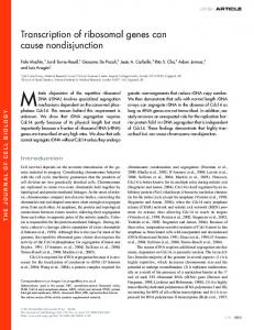
CanTechnology CauseProductivitySlowdowns?*223 Improvements productivity should be interpreted as the economy's ability to produce consumption goods, given values for total inputs. Similarly, we can define output in terms of investment goods, and measure the economy's ability to produce investment goods for given total inputs. This amounts to multiplying the above constraint with yi/y, which yields an output definition which is associated with the productivity level y,. In other words, "aggregate productivity" defined this way really is sectoral productivity, and the aggregate productive ability of the economy is best described by a vector (y,, yc). Thus, the additional theoretical assumptions allow us to recover the sector-specific productivity parameters without the knowledge of sector-specific input levels. Equipped with a standard capital accumulation equation and some specification of savings behavior, we now have a version of the standard neoclassical growth model which allows for investment-specific technological change. As such, this framework is well suited for analyzing the relative importance of investment-specific technological change for longrun output growth. Such an analysis is performed in Greenwood, Hercowitz, and Krusell (1995), and it proceeds in two steps. First, the growth rate of q is identified with the rate of decline of the relative price of capital goods, as given by Gordon's price deflator for PDE divided by the price deflator for nondurable consumption goods and services.16 The updated version of this series is plotted in Figure 2. According to Figure 2, the relative price of PDE declines (that is, investment-specific technological knowledge increases) at an annual rate of about 3%. Also, it appears that the rate of price decline is larger towards the end of the sample, and that the change in trend occurs in the mid-seventies. We will get back to this issue shortly. Second, the growth rate of this ratio over the sample is used to calculate how the long-run growth rate which follows from the balanced-growth path of the model depends on the two kinds of investment-specific and neutral technological change, respectively. Greenwood, Hercowitz, and Krusell (1995) find that the former accounts for around 60% of total consumption growth, which is what is of importance to consumers living in this kind of economy. As part of the procedure, a series for the neutral technological change z is obtained. The series is displayed in Figure 3. This graph shows a drastic version of the productivity slowdown: neutral productivity increases until the mid-seventies, after which it falls uninterruptedly until the very end of the sample, when it increases again. There are two reasons for the drastic productivity slowdown/fall. The first reason is the increase in the rate of growth of the capital stock 16. That analysis also distinguishes between investment in PDE and in structures.
224 * HORNSTEIN & KRUSELL Figure 2 PRICE OF PDE RELATIVETO NONDURABLE CONSUMPTION AND SERVICES 1.21.0
0.8 0.6 >
0.4
-_ 0
0.2 0.0 -0.2'
-0.4
1960
1970
1980
1990
Year
Figure 3 NEUTRAL TECHNOLOGICAL CHANGE
0.0
-
0.25 ' \.\
0.20-
0.10 o
\ -
. /
'\'
0.10
-/
-
0.05 -
- q, unequal factor income shares ._ 1 /p, or q with equal factor income shares
/
0.00 1960
1970
1980 Year
1990
CauseProductivity Slowdowns??225 CanTechnology Improvements implied by Gordon's revisions of the relative efficiency of new investment. Second, we measure the economy's current ability to produce nondurable consumption goods and services, but these goods are to a large extent supplied by the unmeasurable sector. We have seen above that TFP in that sector actually declined in the postwar period, and thus our result is perfectly consistent with the sectoral revisions above. To evaluate the economy's ability to transform current consumption into future consumption, the growth of q becomes relevant.17 This paper examines possible implications of investment-specific technological change for productivity accounting. In particular, we use theoretical model economies to examine whether this phenomenon, together with learning about new technologies and mismeasurement of the quality improvements in new goods, can help us understand the recorded productivity slowdown. Before we proceed to that analysis, however, we have two more topics to cover. As a background, we will first provide a brief review of explanations for the productivity slowdown. Second, we take another look at technological change occurring in the investmentgoods sector and provide some additional evidence that the rate of investment-specific technological change has increased sometime during the mid-seventies. 2.3 EXPLANATIONS FORTHESLOWDOWN:A BRIEF REVIEW LITERATURE A variety of explanations have been proposed to account for the productivity slowdown. At this point we provide a brief review of the more popular ones. We would like to suggest that while these explanations account for some of the observed slowdown in TFP growth, the larger part of the slowdown remains unexplained. The review will be quite brief and sketchy. For a more comprehensive treatment the interested reader may consult any one of the many excellent survey papers, summaries, and conferences volumes on the subject.18 A reasonably comprehensive list of potential explanatory factors is as follows. We exclude the "measurement explanation" here, since it has already been discussed and will be elaborated on in later sections. Decreases in labor quality. In the productivity calculations above, no adjustments are made for changes in labor quality. Many authors have 17. Note also that the abilityto produce durableconsumptiongoods is not directlygiven by the graph, but needs to be adjustedby the relativepriceincreasefor nondurablesin terms of durables. 18. See, for example, Cullison (1989),the 1988:2(4)issue of the Journalof Economic Perspectives, and Baily and Gordon (1988).
226 *HORNSTEIN& KRUSELL used educational attainments, possibly corrected for the quality of the educational achievements (e.g., as measured by SAT test scores), and other aspects of changes in the heterogeneity of the labor force (the age-race-sex distribution) to revise the labor input. The difficulty with this explanation is that no substantial changes in the labor input can be detected at the time the slowdown began. In addition, many of the changes in the quality of the labor force are specific to the United States and therefore do not explain the international slowdown. Views on the importance of this explanation, however, differ.19 The oil shock(s). To many, the most attractive explanation for the slowdown is the oil shock, because the timing is right and because it is common to all countries.20 There are problems with this explanation. Taking into account the cost share of energy, and the modest slowdown that occurred in actual energy input, only a very small fraction of the slowdown can be accounted for. Indirect effects through capital obsolescence are also problematic: given the small energy cost share, the massive move to alternative kinds of capital which would be needed to motivate the large slowdown seems to contradict profit maximization. In addition, we have not observed the changes in usedcapital prices that would follow from the obsolescence explanation. Furthermore, following the reduction in real oil prices in the eighties we have not observed an increase in TFP growth rates which is comparable in magnitude to the slowdown in the seventies. All the same, the timing of this explanation is "too good to be a coincidence" in the views of many, and other indirect, but not spelled-out effects, such as macroeconomic disruptions, have been mentioned.21 A slowdown in R&D and the number of technologicalinnovations. In the United States, the R&D share of total expenditures declined in the mid-sixties, and the number of patents per R&D dollar has also declined. However, the decline in R&D expenditure is specific to the United States, and R&D expenditures have increased again without a concomitant increase in productivity. Moreover, the R&D explanation is tailored to the manufacturing industry, and does little to address the decline in service-sector productivity. Did the number of new innovations go down, and are we experiencing diminishing returns to R&D and "technological exhaustion"? First, in the United States the decline 19. For references, see Denison (1985), Darby (1984), Baily (1981a), Baily and Gordon (1988), Jorgenson et al. (1987), and Dean, Kunze, and Rosenblum (1988). 20. Baily and Gordon (1988) do provide an argument why the timing is not perfect: a slowdown had already begun in several sectors before the oil shock. 21. For references, see Nordhaus (1982), Summers (1982), Baily (1981b), Jorgenson et al. (1987), Bruno (1981), Bruno and Sachs (1982), Hulten, Robertson, and Wykoff (1989), and Olson (1988).
CauseProductivity CanTechnology Slowdowns?*227 Improvements in the number of granted patents can be explained by budget cuts and a decline in resources allocated to patent granting. Second, in our view, it seems difficult to argue that the last two decades have been characterized by particularly slow technological change, considering the rapid expansion in information technology and other hightechnology areas.22 Regulations, cultural change, labordisputes, managementfailures. It has been argued that the increase in the number and strictness of regulations in the United States during the second half of the postwar period may have played an important role in lowering productivity. Similarly, there have been increases in crime rates and labor-market disruptions which have the potential to lower productivity. Management failures which could also be reflected in a decrease of measured productivity have also been stressed. Although there are merits to all these explanations, they have the usual problems: there is no perceived sharp increase in any one of these factors in the mid-seventies, and although some of these problems did occur in some other countries, none of them is worldwide.23 The coincidenceof a number of sector-specificproblems. One approach is to analyze what might have caused the slowdown sector by sector. For example, it has been argued that the slowdown in construction is due to unionization, as well as to specific problems with output deflation. Mining has had problems because marginal costs of extraction have risen rapidly, especially during the time the oil price and production increased. The electric utility industry is characterized by large fixed costs and very low marginal costs, so when demand decreases, as it did after the oil shocks, measured productivity falls substantially. Although some of the sector-specific explanations have common causes, such as the oil shocks, a more complete analysis of all sectors is unlikely to satisfy the timing requirement and to be valid for other countries.24 In conclusion, views differ widely on the quantitative importance of the different explanations for the slowdown. Denison (1985) can account 22. For surveys and case studies on R&D, see Griliches (1988, 1994) and Baily and Chakrabarti (1988). For the technology exhaustion hypothesis, see Baumol and Wolff (1979), and Nordhaus (1982). 23. For references on the effects of regulations, see Denison (1985), Norsworthy, Harper, and Kunze (1979), and Christiansen and Haveman (1981). For cultural aspects, see Denison (1985), and Naples (1988). For labor-market disruptions, see Denison (1985), Gordon (1981), and Naples (1981), and for management failures see Hayes and Abernathy (1980), Dertouzos, Lester, and Solow (1990), and Summers (1982). 24. For references, see Baily and Gordon (1988), Allen (1985), and Thurow (1987).
228 * HORNSTEIN & KRUSELL
for about one-third of the slowdown in the seventies with a subset of the explanations listed above. Others claim greater success, but it seems fair to say that not more than half of the slowdown has been accounted for. 2.4 EVIDENCE ON STRUCTURAL CHANGE
We propose an alternative explanation of the productivity slowdown: we suggest that the measured decline in productivity growth can in part be attributed to an increase in the rate of investment-specific technological change. In this section we present evidence for an increase in the rate of investment-specific technological change during the seventies. In the next sections, we will then discuss why an increase in the rate of technological change may lead to a decrease in measured productivity growth. Because technologies are available worldwide, our explanation can account for the simultaneous decline in productivity growth among industrialized countries. The task of quantifying the rate of technological change, not to mention detecting a long-term change in this rate, is difficult. There is ample anecdotal evidence on important technological improvements, most of them capital-embodied, which have occurred during the last decades. Many of these improvements have been associated with the introduction of microprocessors and computers into the production process. Computers have made possible new organizational structures, and they have been incorporated into other capital goods. In manufacturing, numerically controlled machine tools, robotization, and automatic assembly have been introduced in many production processes [see Edquist and Jacobsson (1988) for a discussion]. Faster and more efficient means of telecommunication and transportation have also been developed. It is of course difficult to date any of these developments precisely, but many of them did appear in the seventies. Of course, the critical reader should then note that the fifties and sixties also saw many advances in the production of consumer electronics, cars, and so on. Although most of the anecdotal evidence which we have encountered for the earlier period is less equipment-related than for the period of the slowdown and thus not really contradictory with our thesis, it is clear that we need to go beyond speculation about an increase in the rate of capital-embodied technological change based purely on anecdotes. Therefore, we investigate two measures of the aggregate rate of investment-specific technological change. These measures are based on different kinds of data, and thus complementary. They do speak in favor of a structural break in the growth rate of capital-embodied technology.
CauseProductivity CanTechnology Slowdowns?*229 Improvements 2.4.1 Use of the Relative-Price Data Hulten (1992) and Greenwood, Hercowitz, and Krusell (1995) identify the growth rate of capitalembodied technological change with the rate of decline in the relative price of investment goods. Their procedure, as outlined in Section 2.2.2, relies on assumptions similar to those in Solow (1957). The relative price of PDE based on Gordon's price series is displayed in Figure 2. Inspection of this figure suggests that starting in the mid-seventies the relative price of new capital declined at a higher rate, about one percentage point more on an annual basis. This would indicate an accelerated rate of capital-embodied technological change. Before we test for a structural break in the relative-price series, we want to discuss in more detail the identification of the relative price of capital with capital-embodied technological change. A change in a relative price can reflect a change in relative productivity, or it may simply reflect substitution in production. The analysis in Section 2.2.2 shows that the relative price of investment goods reflects the relative productivity of the investment sector only if production is competitive, inputs are mobile across sectors, and the production isoquants are the same in the investment- and the consumption-goods sector. In terms of a Cobb-Douglas production function, the last condition means that the capital and labor income-share parameters have to be the same. As we have pointed out earlier, income shares differ across sectors; in particular, the sector producing durable goods has one of the lowest capital income shares. Greenwood, Hercowitz, and Krusell (1995) show that on the balanced-growth path the behavior of the relative price of investment goods depends crucially on the relative income shares in the consumption- and investment-goods sectors. In particular, if the capital income share is lower in the investment sector and there is no investment-specific technological change, we should observe an increase in the relative price of investment goods. Since we observe the opposite, the decline in the relative price of investment goods must underestimate the growth rate of investment-specific technological change. More to the point, to the extent that income shares in the two sectors are different and trend differently over time, any inference about the rate of technological change which assumes constant and equal shares will be misleading. To be more concrete, assume that production in the investment- and consumption-goods sector is Cobb-Douglas, Ct
-
lkac,tll-ac,t " t"'c,t "c,t
it =qtzk ;i, t
Cit
230 *HORNSTEIN& KRUSELL and that income shares are not constant. Assume perfect competition in production, and let Ptdenote the relative price of capital. It is easy to show that the relative productivity of the investment-goods sector qtsatisfies the following relationship when inputs are freely mobile across sectors: 1 Ct
C ktijll- ai,t ,t t "i, ' -c,t ' 1ac't-a"ct it k'c,t
qt
where kt = kc, + ki, and I = lt + li,tand
1+ =
It ptit1 ai,t Ct 1 - ac,t
and kt
kt =ct
1 1+
-7ac,t ai,t i,t 1 - ti,taC,tIc,t
Using data on aggregate quantities {kt, lt, ct, it}, prices {Pt}, and income shares {atc,, at}, we can use these equations to construct a series for the relative productivity of the investment sector, qt. In particular, we use time-series data on the capital income share to isolate the effect of any trend change in this variable on the relative price.25In the postwar United States the capital income share in the durable-goods manufacturing sector has declined relative to the share in other sectors. Following our argument above, everything else equal this should lead to an increasein the relative price of equipment. Hence, our adjustment procedure will imply an increasing trend in the rate of investment-specific technological change. The reciprocal of the relative price Pt and our measure of investmentspecific technological change qt are graphed in Figure 4. The price of PDE relative to the price of nondurable consumption and services declined over the postwar period, and the rate of this decline increased in the mid-seventies. A simple regression of the relative price of PDE on a time trend and a change in trend in 1973 shows that there was a 25. In the actualimplementation,we have used a slightlymore elaboratesetup which uses both equipment and structures,and the investment sector thus representsthe sector producing equipment. For a more detailed descriptionof the data and the procedure used, see the Appendix.
CauseProductivity Slowdowns?*231 CanTechnology Improvements TECHNOLOGICAL CHANGE Figure4 INVESTMENT-SPECIFIC 15 1.3
,-
q, unequal factor income shares ._ 1 /p, or q with equal factor income shares
1.1 0a
0.9 -
-)
1
0.-7 0.7 00 0.5-
_j
0.5 -
0.3 0.1 -0.1
1960
'.
I
1970
1980
1990
Year
statistically significant increase in the rate of decline from 2.9% before 1973 to 3.6% after 1973; see column 1 of Table 7. In the second column of Table 7 we present the results from a regression of the derived inverse relative productivity series on a linear time trend with a change in trend in 1973. The derived inverse relative productivity series exhibits an even faster rate of decline, and the rate of decline increases from 3.2% before 1973 to 4% after 1973. The change in the rate of decline is highly significant. Finally, we should comment on the assumption that prices are given by marginal productivities. If markups are variable, changes in relative prices need not reflect relative productivity change. It is thus possible that the decrease in the rate of decline of the relative price of equipment reflects a decline in markups. This is consistent with the notion that we have seen an increase in international competition for at least a subset of the economy's products. However, note that for this alternative explanation of the structural change in the relative-price time series, two elements are necessary. First, it is necessary that the decline in markups have the right time-series pattern. In particular, to explain the change in the trend of the relative price around the mid-seventies, the markup would need to have started to fall around the same time, and it would need to have continued to fall throughout the rest of the period (actually, the fall in the relative price even seems to accelerate toward the end of
232 *HORNSTEIN& KRUSELL Table7 STRUCTURAL CHANGE Dependent variable
Constant Trend Trend change for t - 1973
log Pt
log (llqt)
0.0415 (0.0204)a -0.0289 (0.0014)b
0.0569 (0.0169)a -0.0322 (0.0012)b
-0.0058
-0.0085
(0.0026)a
(0.0021)b
asignificantat the 5%level. bsignificant at the 1% level.
the period). Second, it is necessary for the decline in markups to have been larger for equipment goods than for consumption goods, since otherwise there would be no change in the relativeprice which we focus on. Although we do not suggest to rule out the declining-markup explanation, we do not know of any evidence supporting the necessary elements for this explanation. 2.4.2 Other Evidenceon Capital-EmbodiedTechnologicalChange The literature on vintage-specific productivity effects can also be used to shed light on the rate of capital-embodied technological progress. In fact, McHugh and Lane (1987) looked at precisely the issue we are interested in. They study the effect of the age of capital on labor productivity using data from two-digit manufacturing industries in the United States. Using a framework which builds on Solow (1959), they conclude that (1) labor productivity declines significantly with increasing age of the capital stock, and (2) the negative effect of the age of capital is significantly stronger for capital installed after 1974. That is, a one-year difference in capital vintage corresponds to a larger productivity difference if the capital was installed after 1974. McHugh and Lane hence conclude that there was an increase in the technological advancement embodied in capital. The results of McHugh and Lane are derived from a model structure and a concept of technological change quite like ours, and they are consistent with our findings. Their results provide additional, independent evidence for our hypothesis of an increase in the rate of investmentspecific technological change sometime in the mid-seventies.
3. Theoretical Framework andAnalysis The increase in the rate of investment-specific technological change can reduce measured productivity growth for several reasons. A higher rate
CauseProductivity Slowdowns?*233 CanTechnology Improvements of technological change means that new technologies with which producers have less experience are introduced at a faster rate. This can lead to temporarily lower output growth. Moreover, it causes problems for productivity measurement, since experience is unobserved. Faster technological change can also mean that new kinds of goods which differ substantially in their characteristics from existing goods are introduced at a faster rate. This makes the measurement of output more difficult. There is a substantial body of research which shows that learning, in particular learning by doing, has important effects on productivity. Over time individuals learn how to perform certain tasks, production sites become more efficient, and productivity increases. Learning curves which relate productivity to some measure of accumulated experience have been estimated for a large number of applications: well-known examples in economics include Rapping (1965) on shipyards and Alchian (1963) on airframe production.26 While there is agreement on the fact that there is learning, there are few explicit models of the learning technology itself.27 In our work we will simply assume that learning about new technologies is necessary and that it is exogenous. We will study the quantitative implications of learning for the measurement of productivity growth in a simple vintage model of growth. In previous sections we have argued that for a large part of the economy measures of output are not reliable. We will develop a simple model in which we can discuss the problem of mismeasured output and how it relates to an accelerated pace of technological change. Again, the purpose is to quantify the implications for the slowdown of productivity growth in a simple vintage model. In a final section, we bring the two explanations of the productivity slowdown together, and we use actual United States input and relative price series for a quantitative evaluation. 3.1 SLOWDOWNSDUE TO LEARNING We now turn to productivity measurement in a growth model when there is learning about new plants or new capital goods. Suppose that any investment in period t is incorporated into a "vintage t" plant. In other words, we do not consider "retooling." In each existing plant learning proceeds at an exogenous rate. The production function with learning thus reads y = yTkll-a, 26. For a survey on learning by doing in the management literature see Yelle (1979). 27. Recently Jovanovic and Nyarko (1995) have interpreted estimated learning curves within a Bayesian learning model.
234 *HORNSTEIN& KRUSELL where T represents what has been learned about the plant, and T is increasing with time. It is possible to think of the structure in this section as the consumption-investment two-sector model of Section 2.2.2 with y here representing sector-neutral technology (y,), and so on. 3.1.1 A Vintage Model with Aggregation At time t, total investment is it, and it is all put into a new plant (or many smaller plants). With the assumption that each unit of capital depreciates at rate 8 per period, the output at time t of a plant which was set up with investment in t - ', which we label Yt,, is t-t( [i y tTt,
Yt,r
-
8)r-1]
l
a
for all t and all r > 1, where Tt, is the experience level and t,, the amount of labor used at this plant. Total production of goods is Yt =
Yt,t
T =1
When labor can be allocated freely across vintages at any moment in time, optimal allocations satisfy It, = lt,lrt,/
where
Tt
it-Tr
This condition follows from equalizing the marginal product of labor across plants. The vector (1, r,2, rt3, . . .) thus describes the relative allocation of labor across vintages and, in particular, across learning levels. Using the resource constraint for labor, it is straightforward to show that it It,1
-
I ZT=lrr,,r
where lt is the total amount of labor input at time t. Similarly, total output at time t satisfies ytktl-a */(= 7^t Yt
t '1
CanTechnology CauseProductivity Slowdowns?*235 Improvements where 00
kt=
T7=1
-1ltT
itl-y(1
Hence, this economy admits sectoral aggregation: there exists an aggregate capital measure kt, defined as above, such that output at any point in time is given by a function of this capital measure, total labor input, and the productivity parameter alone. It is clear from the above that if there were accurate measures of the learning parameters Tt,,, aggregate growth accounting would proceed as in the previous section, replacing the total capital stock ktwith kt, and the TFP growth rate would be A log zt = A log Yt- a A log kt - (1 - a) A log lt. This procedure would indeed lead to accurate measurement of technology change: A log zt = A log yt. Instead, however, we assume here that capital is measured as in the national accounts, which do not adjust for learning levels. Thus, the measured capital, kt, is calculated using kt+ = (1 - S)kt+ it, so that
kt=
T=1
it.(1
-
8
1,
and growth accounting results in measured TFP growth log zt = A log yt - aA log kt - (1 - a) A log
It.
For this analysis, we assume that output and labor input are well measured. Given that learning levels are not well measured, however, there is no reason to expect that A log zt = A log zt in general. On a balanced growth path, however, the growth rate of productivity is accurately measured. Specifically, suppose that yt = yt and that investment-specific technological change is given by yqt = y' so that output in consumption units grows at
y1/(1-a)^ya0(l-a)
and investment
and capital at
(yyq)l/'-a).
It is
easy to see that in this case the vector rt, has to be constant over time, independently of the assumed learning process. Hence, the discrepancy between ktand ktis constant over time, and it follows that A log kt = log kt.
In the following experiment, we represent structural change by a onetime permanent change in the growth rate of yqt. More specifically, we assume that the economy is on a balanced growth path with both sources of productivity growing at constant rates, but that the rate of
236 - HORNSTEIN& KRUSELL investment-specific technological change increases once and for all, whereas sector-neutral technological change stays the same. For this experiment, we use the actual pre- and post-1973 growth rates calculated in Section 2.4. This experiment will lead to changes in the measured growth rate of TFP, A log z, even though the true growth rate is unchanged. The mismeasurement is temporary: as the economy converges to the new balanced-growth path, the error converges to zero. The parameters are calibrated as follows. We choose a = 0.3, 8 = 0.1, an investment rate of 0.12, and y = 1.01. The initial value for yqis taken to be 1.032, and its new value 1.041. The learning technology is specified as Tt7 = 1 - A-l(
- Tt,,),
that is, learning is geometric with convergence rate A from a starting value of Tt,1.We consider two ways of selecting the starting values. First, we look at constant starting values. Following the study by Bahk and Gort (1993) of the long-term experience accumulation in new production plants, we chose A = 0.7 and T, = 0.8. Compared with most of the empirical literature on learning, these values imply a relatively slow learning rate and a small scope of learning. This literature, however, has typically been focused on well-defined learning tasks and not dealt with the kind of complex learning that is a likely result of the technological change we consider here. We actually consider our calibration conservative, since for example the organizational changes in the workplace implied by the availability of information technology (IT) seem more complex and costly than the learning processes analyzed in Bahk and Gort (1993). Moreover, it is arguable that the new information and telecommunication technologies introduced since the seventies have incorporated a new kind of learning or adjustment element because of network externalities: firms do not benefit from and cannot fully learn about their new investment goods until other firms invest as well. Second, we consider the starting value to be a function of the rate of investment-specific technological progress. In the context of IT investment, Yorukoglu (1995) argues that there are important compatibility problems across different types of capital. In particular he suggests that the more advanced the new equipment is relative to existing equipment, the lower is the initial experience with the new equipment. We consider it reasonable to adopt this approach also when capital is defined more broadly. To simplify things we assume that at the time the rate of investment-specific technological change increases, the starting value for experience declines to Tt,1= 0.6.
CanTechnology CauseProductivity Slowdowns??237 Improvements Figure5 LEARNING (b) Solow Residuol
(o) Output Growth 3.2 -
1.002 -
3.1l 3~
?
_
0.992 -
/
? 3.0 -
/
0O~~~.
0.982-
I./z
o
o
2.9 -
S/Leo~~
2. 82.7
2.BS"~~~~
-
Xe
0.972-
. 0
. 10
. 20
. 30
. 40
50
60
0.962
0
.
.
.
..
10
20
30
40
50
60
Period
Period
(c) Productivity Level 150 140 -
130
o 120
0
J
110 100
90
0
10
20
30
40
50
60
Period
3.1.2 Results Our results for the two cases are displayed in Figures 5 and 6. Figure 5 assumes no compatibility problem, whereas Figure 6 does. Common to these figures is an initial slowdown and a subsequent recovery of measured TFP growth, Az. Note in Figure 5, however, that for the learning parameters we selected, there is no slowdown in output growth. Since total employment is fixed, this also means that there is no slowdown in labor productivity growth. Only with a compatibility problem do we observe a slowdown in output growth. The slowdown in productivity growth reflects reallocation of labor toward more recent vintages due to the higher rate of technological progress, and with more labor concentrated in recent vintages, average learning factors necessarily drop. Notice also that with a compatibility problem the decrease in the average learning level among plants causes a permanent level drop in measured TFP, even though the TFP growth rate comes back to its true value. The model with a compatibility problem does produce a noticeable slowdown: measured TFP growth declines by 11 percentage points. However, the slowdown is short-lived: it lasts no longer than 5 years.
238 *HORNSTEIN& KRUSELL PROBLEM Figure6 LEARNINGWITHA COMPATIBILITY (b) Solow Residuol
(o) Output Growth
-
3.2 -1.0 > 3.0 -
0.8 0.6
2.8< 2.4 o u
2.2 2.018-
o
:: 1.4
.
~~~~~~~2.4
?* ?--~0.4
/
/ o
-
/
1.2 1.0 -
/
/
0.2 0.0 -
-0.2 -0.4 -0.8-
0
10
20
30 Period
40
500
40
50
0 0
20
30 Period
0
50
60
(c) Productivity Level 10
-
140 1 30 o
/
$
120 -
.J
110
-
100 90
0
10
20
30 Period
60
We have also used our learning formulation to adjust actual United States capital stock data by sector, which allows a revision of the TFP figures. The revisions, which are based on the same parameters as Figure 6 and which also use capital stocks based on Gordon's price-index data, are displayed in Table 8. The adjustment of the capital stock for learning increases measured TFP growth. The effect is not particularly large overall, on average about 0.2 percentage points for the 1954-1993 period. For the productivity slowdown of the mid-seventies, the effect is more substantial. Overall measured TFP growth for the 1973-1979 period is about 0.7 percentage points higher than without an adjustment for learning, with the most dramatic effect on finance and insurance, where TFP growth is now about 1.2 percentage points higher. We also include numbers for the measurable and unmeasurable sectors as defined in Section 2.1. The adjustment of the capital stock for learning affects measured TFP about the same way in the measurable and unmeasurable sector. Learning alone has a small effect, increasing measured TFP growth by about 0.1
CanTechnology CauseProductivity Slowdowns??239 Improvements FORLEARNING Table8 TFPGROWTH,1954-1993WITHADJUSTMENTS Growthrate(%) Sector
54-93
54-73
73-79
79-93
Totalprivate sector Agric., forestry, fishing Mining Construction Manufacturing Durables Nondurables Transport.,publ. util. Wholesale trade Retailtrade Financeand insur. Other services
0.9 0.6 -0.7 -1.3 2.6 3.6 1.6 2.1 1.4 -0.2 -2.2 -0.9
1.4 -0.4 0.5 -1.8 3.2 4.1 2.4 2.8 1.1 -0.0 -2.1 -1.0
0.2 -2.4 -8.4 -2.2 1.7 2.2 1.0 1.0 0.9 -0.1 -0.5 0.4
0.5 3.3 1.1 0.0 2.3 3.5 0.6 1.6 2.0 0.0 -3.0 -1.3
Measurablesector Unmeasurablesector
2.1 -0.7
2.6 -0.7
0.7 -0.3
2.2 -0.8
percentage point overall; but correcting for a compatibility problem during the 1973-1979 period increases measured TFP growth by about half a percentage point. Moreover, the measurable sector appears to be more affected by this correction than the unmeasurable sector. An increase in the growth rate of investment-specific technological change is not the only possible trigger of a learning-induced slowdown in productivity growth. Our argument can be also applied to an investment boom whether or not this boom is associated with technological change. For example, Young (1992) documents that Singapore experienced considerable growth in investment rates and capital accumulation, but no recorded TFP growth.28 From our perspective, rapidly increasing investment would induce a decline in recorded TFP growth, and given the magnitude of the increase in capital accumulation in Singapore, zero measured TFP growth does not seem surprising. In contrast, however, note that an increase in the capital stock which results from an increase in the rate of technological change would be more severe, since it would also involve compatibility problems between new and old technologies.29 28. Investmentrates increasedfrom 9%of GDPin 1960to 43%of GDPin 1984. 29. As a gauge on the role of the assumptionthat laboris freelymobileacrossvintages, we also considered the vintage formulationused in Cooley, Greenwood, and Yorukoglu (1995).With the same setup as above, suppose that once capitalis allocatedto a plant,
240 - HORNSTEIN & KRUSELL 3.2 SLOWDOWNS DUE TO QUALITY MISMEASUREMENTS
We have argued that for most industrialized economies the unmeasurable sector, that is, the sector where output is badly measured, is large. There is a presumption that we underestimate output growth in this sector, because it is more difficult to capture quality changes of goods in this sector. We now describe a simple model in which output does have a quality and a quantity component, and we make the extreme assumption that we can only measure the quantity component of output. We then study the quantitative implications for productivity measurement when the rate of investment-specific technological growth changes in the model economy.30 We formalize the distinction between the quantity and quality components of output by identifying each component with a separate production process. We thus postulate that output y at a plant can be decomposed to read YQ, where Y is the number of goods, which is well measured, and Q is a one-dimensional quality index per good, which is not measured at all. Capital and labor are inputs to the production of quantity and quality Y=
(ykyl
a
and
Q=
(ykQl-aQ
and the capital intensity (share) in the production of quantity and quality may differ. The parameter 13represents the relative quantity content of the output. Note that the production technology for output measured in quality units has constant returns to scale in the capital and labor init remains there until the plant shuts down, at which point capitaldepreciatescompletely. Also suppose that each plant has a fixed laborrequirementof one. All laboris paid the same wage rate, and capitalis allocatedto a plantuntil the presentvalue of the sequence of marginalproducts of capitalequals the currentcost of investment. There will be a point at which a plant shuts down, since the marginalproduct of laborin a given plant will grow at a slower rate than the wage rate. In order to simplify the characterizationof the optimalinvestmentdecision, assume also that the interestrateis constant. A balanced-growthpath for this economy can be summarizedby (1) a constant growth ratefor the wage rate, and (2) a fixed life span of plants. The wage rateat a point in time has to be such that the oldest vintage finds it profitablenot to close down. Finally,the amounts of investment and laborattractedto new plants have to be such that present-valueprofitsare zero when the total amountof laborhired for new plants equals the numberof laid-offworkersfrom old plants shutting down. Our analysis of this model frameworkleads to results which are very similarto those obtainedin the model with aggregation.The qualitativefeatures of the model are the same, and the quantitativeresults from the same set of parametersfor learningare also very similar. We detected the largestdiscrepancyin the averageage of firms,but this differencewas not large enough to generatesignificantlydifferentaggregateoutput paths. 30. For a related analysis of unobserved quality in an endogenous growth context see Howitt (1995).
CanTechnology CauseProductivity Slowdowns?*241 Improvements puts.31 We assume that in the national income accounts of this model economy only the quantity component of the consumption aggregate is measured, but that investment goods are well measured. We will model structural change in two complementary ways, and each way has different implications for quality mismeasurement. First, we will consider the kind of experiment that we studied in the previous section: at a point in time, the growth rate of investment-specific technological change increases permanently. Second, we consider an experiment where this technological shift also leads to a relative shift toward quality production. We now develop the specific time-series implications of the experiments, first by considering the mismeasurement on the plant (vintage) level, and then on the aggregate level. 3.2.1 Quality Mismeasurement on the Plant Level Consider an isolated production facility, and note that the optimal allocation of a given amount of capital k and labor I across quantity and quality production has to satisfy ky
_
kQ
8
--ay 1 -paQ
3 1 - ay -IQ= ly 1 - p1 - aQ
and
where ky + kQ= k and ly + IQ= 1. This implies, after some manipulations, that total output can be written y = Ayk"ll-a,
where a -= 3ay + (1 - P)aQ and A = AyAQ,with
r
y
ay
/3(1
- ay) '_ y
and A [I (1 P) aI
Q(
(1 - P)(1
(1-
a)
Q)
1-aQ ]1-
J
31. The constant-returns-to-scale property is assumed for convenience: it greatly simplifies decentralization of the model, and it allows the identification of relative prices with marginal products. However, it does carry some features which for several examples may appear unrealistic. First, the production of quality can often be thought of as a process where resources are devoted once and for all to develop a new product which will be available forever. Second, by implication of our formulation, if no effort (input) is devoted to quality production, then nothing is produced.
242 *HORNSTEIN& KRUSELL Furthermore, the subcomponents of output satisfy Y = Ay (ykaY'1-Y)
and
Q = AQ (ykaQ1-aQ)1-.3
Parenthetically, notice from these facts that if both quantity and quality are well measured (and there is no unobserved learning), then standard growth accounting allows growth in y, A log z, to be measured perfectly. In our economy the national income accounts use quantities only to measure total output growth: A log Yt = 8 [A log z, + ayA log k, + (1 - ay) A log t], so that measured TFP growth, A log z, is A log
Zf = A log Yt -
A4log k, - (1 - a) A log I.
It is important to note that the total capital share, a, is used in this calculation. From the last two equations it follows that A log 2, = -
A log z, - aQ(1 -
3) A log k, - (1
-
aQ)(1 -
S) A log It.
There are several important characteristics of this equation. First, if / = 1, so that there is no quality component, then clearly z would be accurately recovered with the growth accounting procedure. Second, if 3 < 1, then so long as all variables grow, productivity growth is underestimated because of quality improvements: A log z < A log z. Moreover, an increase in the rate of growth of capital will increase the mismeasurement. So when the growth rate of investment-specific technological change increases, there will be more than a one-to-one increase in the growth rate in the capital stock, leading to a slowdown in measured productivity. Notice that for this result to obtain qualitatively, all that is needed is that some of the capital is used in the production of quality (i.e., our assumption that the capital share is equal in the production of quantity and quality is not crucial).32 Third, for a given 3 and a, measured productivity growth underestimates actual productivity growth more the higher aQ is relative to ay, i.e., the more capital-intensive is quality relative to quantity production. An example where aQ would be large can be found in banking services, where the introduction of computers has added significant convenience for the customer in the ability to quickly obtain information, move funds across deposits, make payments, and so on. Yet the quantity output, 32. In contrast,Howitt (1995)assumes that qualityis a functionof "knowledge,"and not a direct functionof capitaland labor.
CanTechnology CauseProductivity Slowdowns??243 Improvements which may be measured as the number of deposits, is probably more directly related to the number of bank employees.33 Fourth, notice that the time path of the measured productivity growth rate will be monotone in response to a one-time, permanent increase in the growth rate of investment-specific technological change. To see this, note that the increase in the latter will cause the capital stock to grow faster, in a monotonic way, toward its new growth rate. Since the underestimate is directly proportional to the growth rate of the capital stock, A log z will decline monotonically to its new value. As we shall see, this result will be overturned when we consider the aggregation of mismeasurements over plants/vintages. In quantitative terms, it is possible to calculate the maximal measured (long-run) productivity slowdown due to our hypothesis of an increase in the growth rate of capital as follows. First, without restrictions on a or 13,the largest possible slowdown would obviously equal the increase in the growth rate of capital (setting , = 0 and aQ = 1). However, restricting this estimate by the observed total capital share of &, the maximum bias from a one-percentage-point increase in the capital stock growth is given by a itself, which can be achieved either by setting 3 = 0 and aQ = a or by setting aQ = 1 and /3 = 1 - a. As an example, a one-percentage-point increase in the growth rate of investment-specific technological change together with a capital share of 0.4 implies a 1 x 1/(1 - 0.4) increase in the long-run growth rate of the capital stock, and the maximal long-run slowdown in productivity is therefore 0.67%. 3.2.2 The Aggregation of Quality Mismeasurementover Plants Now suppose, in line with the formal structure of Section 3.1.1, that aggregate output is produced in plants with different capital vintages. Then we know from the plant level analysis of quality mismeasurement above that correctly measured output at time t in a T-year-old plant satisfies Yt,, = Aytt,'t,l
but that measured output at this plant,
t = Y,,, is given by
=,T =Ayytkt,tT A( (vtkI'ay t.)-y YAT.
The allocation of labor across plants here is parallel to that in Section 3.1.1, so that It, = rt,it = Itrt,/Jlrt,s. It follows that aggregate output 33. In the U.S. national income accounts, measured bank sector output is mainly based on employment data, and not on deposit counts or volumes.
244 * HORNSTEIN & KRUSELL
satisfies the same expression as in that context. Hence, in the absence of measurement problems, the accounting for productivity growth would be straightforward and not give rise to errors. However, with the lack of measurement of quality on the plant level, aggregate measured output Yt equals S1 Yt,,.Now note that the relative measured output at t in plants t - T and t - 1, respectively, t,
A Y)
Y
Yt1
[it-(1 ll
-1]a
Ay [ytiit:.1-~
y
equals t,y}T
t
t
,
so that
Yt= Yt,
r1 r.
T =1
With the special case of equal capital intensities across quantity and quality production (aQ = ay), this expression simplifies further: Yt=
Ay
1A
E rt,T'
In this case, since all variables on the right-hand side of this equation are true values (not mismeasured), we can compare directly with actual total output, which satisfies a similar equation: Yt = Yt,I
T =1
rtT'
For illustration, let us again focus on the special case when capital intensities are the same. It is clear that since T= r~ = (E=' rt,), we cannot exclude different transitional properties for measured output than for true output (with an = sign, the growth rates of measured output would be 3 times that of true output at all points in time).34Hence, productivity measurement as well will exhibit dynamics which are nontrivially different than those for output. The economic interpretation of the above algebra is as follows. True output in our model has exact aggregation over vintages, so that a monotone increase in the rate of growth of the capital stock resulting from investment-specific technological change will lead to a monotone increase in the growth rate of true aggregate output-due to aggrega34. In the long run, of course, the distribution of labor and capital across plants does not change, and so S= 1 rt, does not change, and measured output will grow exactly at / times the growth rate of true output.
CauseProductivity CanTechnology Slowdowns?*245 Improvements tion (linearity), vintage effects are not present. Measured output, however, is not a linear function of true plant outputs, but a nonlinear one: there are nontrivial vintage effects in the aggregation of measuredoutput over plants. In particular, as we shall see in our examples below, there is an initial slowdown in measured output growth relative to true output growth. Similarly, measured productivity growth will drop more during the first 10-20 years than in the long run. As the increase in the rate of growth of capital is in its initial phase, there is concentration of labor in the most recent vintages, and thus greater weight is placed where the errors are large. Only after substantial time, when the rate of growth is the same in all vintages, will the year-to-year mismeasurement be the same in all vintages, and the underestimate of productivity growth become constant. 3.2.3 Exogenous Changes in the RelativeImportanceof Quality The second expression of structural change that we consider is an exogenous change over time in the quality component. This is a stand-in exercise for developing a richer framework where quality is a state variable, and where a higher rate of technological change can have more fundamental effects on quality production than in our model. In a richer framework, it would for example be possible to better capture how the emergence of computers would orient the allocation of labor more toward quality in the form of the new kinds of services that computers can provide. We do not have direct, aggregate evidence that there has been a shift toward quality. However, postwar patent data suggest that quality mismeasurement may be more important now than it was prior to the seventies. To understand why, suppose that we interpret quality mismeasurement as primarily occurring when new goods are introduced, and note that only patents for new final goods can represent a problem for growth accounting. This is true because any undermeasurement of the output of new intermediate goods will cancel with input underestimates when the same goods are used as inputs. Hence, a shift toward patents for final goods will make the quality mismeasurement more severe. On the basis of patent data from the United States and elsewhere, we split the patents into two groups: patents for new kinds of final outputs, and patents for new kinds of intermediate goods. Figure 7 shows the fraction of total patents which apply to final output goods. The figure reveals a nontrivial upward shift around the mid-seventies both for the United States data and for the international data. Our theoretical experiment, then, is to make the parameter / decrease. This can be viewed either as an increase in the relative importance of quality in general output, or as an increase in the mismeasurement prob-
246 *HORNSTEIN& KRUSELL GOODS Figure7 PATENTSFORFINALAND INTERMEDIATE (n 0 0C'
74
0
0
c
73
0
72 Uc
0
0)
0 0n -4-
/
71
\
, x,
70 /,
-
(D
.
\
n'3)
/.
\
Domestic
c
0
\
69
/ /
/
\
I
s'
_
\
0
a 68
Q) a '3)
0-
67
1960
1970
1980
1 990
Year Solid curve:domestic;dashed curve:all.
lems associated with output. A change in 3 will have two effects. It will imply the desired move toward a larger quality component, but it will also lead to a "reduced-form" productivity increase: recall that the optimal allocation of inputs across quality and quantity components implies that a factor B3(1- 3)l1- multiplies the aggregate production function. To isolate the first effect, we premultiply the production relations of both quality and quantity with the disembodied factor/-8(1 - 3)-(1-~. This way, changes in 13will have no effect on aggregate output as correctly measured (i.e., in quality units), provided inputs are optimally allocated. One aspect of structural change appearing in this way, as opposed to solely through an increase in the growth rate of capital, is that there may be a permanent drop in measured output growth following structural change. If there is a permanent increase in the growth rate of investment-specific technological change but no change in 3, there will be a decrease in measured total-factor productivity growth, but the growth rate of output, and of labor productivity, will increase. This result is due to the simple fact that in our quality framework, where the capital share is positive (indeed the same) across the production of quan-
CanTechnology CauseProductivity Slowdowns?*247 Improvements tity and quality, increases in the growth rate of capital will increase the growth rates of both quality and quantity. However, when the structural dechange is expressed via an increase in the quality component-a crease in ,-there will be a permanent decrease in measured output and labor productivity growth rates. Our particular experiment is to assume a slow diffusion curve for /, letting it move from 0.9 to 0.8 over a period of 10 years (as the rate of investment-specific technological change increases), with the largest changes in , taking place in the middle of this period. 3.2.4 Results We perform several experiments. First, we consider the effect of a permanent increase in the rate of investment-specific technological change in an economy with unobserved quality and no learning, and where the capital intensities in quantity and quality production are equal (ay = aQ). Second, we assume that, in addition to the increase in the growth rate of capital, there is a shift towards a higher quality share Figure8 UNOBSERVEDQUALITY (a) Output Growth (measured)
(b) Solow Residual (measured)
2.9
o
2
0.72
2.8
o o
|
0.70
2.7 0.69
o c u e o
0.71
o, f
2.6
0.68
t 0.67
25 0.66
' 0
2.4
10
20
30
40
50
_
0.65
60
0
10
20
Period
(c) Productivity Level (measured)
o
i
-
2.1
-
1.9
-
1.7
-
1.5
-
1.3
-
1.1
-
I
0.9
-
oo
0.7
e