example of a discrete-event simulation, and explore its regenerative properties. .... converge at rate t?1=3; see Goldsman and Meketon. (1986) and Song and ...
CAN THE REGENERATIVE METHOD BE APPLIED TO DISCRETE-EVENT SIMULATION? Shane G. Henderson
Peter W. Glynn
Department of Engineering Science University of Auckland Private Bag 92019 Auckland, NEW ZEALAND
Department of Engineering-Economic Systems and Operations Research Stanford University Stanford CA 94309-4023, U.S.A.
ABSTRACT The regenerative method enjoys asymptotic properties that make it a highly desirable approach for steady-state simulation output analysis. It has been shown that virtually all discrete-event simulations are regenerative. However, the method is not in widespread use, perhaps primarily because of a di�culty in identifying regeneration times. Our goal in this paper is to highlight the essence of the di�culty in identifying regeneration times in discrete-event simulations. We focus on a very simple example of a discrete-event simulation, and explore its regenerative properties. We show that for our example, it is possible to explicitly determine regeneration times. The ideas that are used to establish this fact might prove useful in identifying regeneration times in more general discrete-event system simulations.
1 INTRODUCTION The regenerative method is based on the notion of identifying times when a stochastic process probabilistically \restarts". It enjoys asymptotic properties that make it a highly desirable approach for steadystate simulation output analysis. When the stochastic process is an irreducible positive recurrent Markov chain on a discrete state space in discrete or continuous time, it is easy to identify regeneration times. In particular, the return times to any xed state constitute regeneration times. It has been shown (Glynn 1994) that all \wellposed" steady-state simulation problems are regenerative. However, identifying the regeneration times for a general discrete-event simulation has proved to be very di�cult. Most discrete-event simulations can be modeled as a generalized semi-Markov process (GSMP); see Shedler (1993) for example. GSMPs with single states
(Haas and Shedler 1987) admit a regenerative analysis. In this case the regeneration times are easily identi ed. However, \most" discrete-event simulations do not possess single states, and one must turn to some other method for identifying regenerations. Glynn (1982) exploited a theoretical device introduced by Athreya and Ney (1978) and Nummelin (1978) to de ne regeneration times in general discrete-event simulations. However, it would appear that identifying such regeneration times in practice is very di�cult. Glynn (1989) gave easily veri ed su�cient conditions for a GSMP to be regenerative or not, but again, identifying the regeneration times in practice appears to be di�cult. Henderson and Glynn (1999) revisit the application of the regenerative method to general discreteevent simulation. They discuss the state of the art in regenerative methodology and discrete-event systems simulation. Furthermore, they are able to formalize the notion that, in the absence of some new idea, the practical identi cation of regeneration times will remain di�cult. Our goal in this companion paper is to highlight the essence of the di�culty in identifying regeneration times in discrete-event simulations. We focus on a very simple example of a discrete-event simulation, and explore its regenerative properties. In Section 2 we introduce the problem of steadystate simulation, and formalize the notion of a regenerative process. We also cover the properties of regenerative steady-state estimators that make the regenerative method desirable as an output-analysis approach. In Section 3 we introduce a simple example of a discrete-event simulation, which is basically a superposition of renewal processes. Then, in Section 4 we explore the structure of the superposition process, and show how one might de ne regeneration times. We also explain why it is di�cult to identify the regeneration times in practice, even for the superposition process.
Section 5 continues the discussion of the superposition example, and in particular, shows that it is in fact possible (from an implementation point of view) to explicitly determine regeneration times. The idea that allows one to do so may apply to more general discrete-event systems, and the implications of this point conclude the paper.
2 THE REGENERATIVE METHOD As mentioned in the introduction, the regenerative method is based on the concept of identifying times when a stochastic process probabilistically \restarts". To x ideas, suppose that W = (W (t) : t � 0) is a stochastic process evolving on some state space S . Let f : S ! IR be a real-valued cost function, and de ne the average cost of running the system W up to time t as Zt �(t) = 1 f (W (s)) ds:
t
0
In great generality, it is known that �(t) ! � as t ! 1, where � is a deterministic constant. This occurs, for example, if W is a positive Harris recurrent Markov chain and f is bounded (p. 154 Asmussen 1987). The steady-state estimation problem is the problem of computing �. Clearly, a reasonable estimator of � is �(t) for some large t. One might then ask how accurate the estimator �(t) is. The regenerative method is one approach to answering this question. De ne a boundary sequence to be a sequence (T (n) : n � 0) of strictly increasing random times with T (0) � 0 and with T (n) ! 1 as n ! 1. A boundary sequence induces a set of (random) cycles C (i) = (W (t) : T (i ? 1) � t < T (i)) for i � 1. De nition 1 We say that W is a regenerative stochastic process if there exists a boundary sequence with the property that the induced cycles are identically distributed and one-dependent.
Remark 1: This de nition is weaker than the classi-
cal de nition of a regenerative process, which requires that the cycles be i.i.d.
Remark 2: The same de nition may be applied to processes (Wn : n � 0) in discrete time by simply
taking W (t) = Wbtc . For i � 1, de ne the \cycle quantities"
Yi =
ZTi
( )
T (i?1)
f (W (s)) ds and
�i = T (i) ? T (i ? 1);
so that Yi and �i are the accumulated cost and length of the ith regenerative cycle respectively. The following result discusses the asymptotic behaviour of the estimator �(t) when W is a regenerative process. For a proof, see Glynn (1982) or Sigman (1990). De ne, for i � 1, Zi = Yi (f ) ? ��i .
Theorem 1 Suppose that W is a regenerative process and f : S ! IR. 1. If E (Y1 (jf j) + �1 ) < 1, then �(t) ! � a.s., as t ! 1, where � = EY1 (f )=E�1 . 2. If E (Y1 (jf j)2 + �12 ) < 1, then p
t(�(t) ? �) ) �N (0; 1) as t ! 1, where �2 = E (Z12 + 2Z1Z2 )=E�1 , ) denotes weak convergence, and N (0; 1) is a standard normal random variable.
The constant �2 is called the time-average variance constant (TAVC) for W and f , and its estimation is the key to obtaining con dence intervals for �(t). De ne Zi (t) = Yi (f ) ? �(t)�i . A reasonable estimator of �2 is 41 �2 (t) = t
X [Z (t)
`(t)?1 i=1
i
2
+ 2Zi (t)Zi+1 (t)];
where `(t) = supfn � 0 : T (n) � tg is the number of complete regenerative cycles in [0; t]. Henderson and Glynn (1999) established the following result relating to the asymptotic behaviour of the estimator �2 (t).
Theorem 2 Suppose that W is a regenerative process and f : S ! IR. 1. If E (Y1 (jf j)2 + �12 ) < 1, then �2 (t) ! �2 a.s. as t ! 1. 2. If E (Y1 (jf j)4 + �14 ) < 1, then there exists a nite (deterministic) constant � such that p
t(�2 (t) ? �2 ) ) �N (0; 1); as t ! 1. An expression for � is given in Hen-
derson and Glynn (1999).
Theorem 2 basically establishes that the estimator
�2 (t) converges to the TAVC at rate t?1=2 .
Other estimators of the TAVC have been proposed. Spectral density estimators of the TAVC typically converge at rate t? where < 1=2; see p. 129 of Grenander and Rosenblatt (1984). For \optimal" choices of the batch size, both nonoverlapping and
overlapping batch means estimators of the TAVC converge at rate t?1=3 ; see Goldsman and Meketon (1986) and Song and Schmeiser (1995). Hence, the regenerative estimator of the TAVC converges faster than either of these methods. Furthermore, one must typically deal with \initialization bias" (see Bratley et al. 1987 or Law and Kelton 1992), whereby estimators of � are biased when initial conditions are not representative of steadystate conditions. In the presence of regenerative structure, a slight modi cation of the estimator �(t) does not su�er from initialization bias. Bias is still exhibited through the fact that the modi ed estimator takes the form of a ratio of sample means, but it is possible to correct for \ rst-order" bias e�ects; see Glynn and Heidelberger (1990), and Henderson and Glynn (1999). Once the regeneration times (T (n) : n � 0) are identi ed, it is relatively straightforward to compute regenerative estimators of � and �2 . In the case that W is an irreducible positive recurrent Markov chain on a discrete state space in discrete or continuous time, the return times to any state constitute regeneration times for the system. However, for more general processes it can be very di�cult to identify the cycle boundaries, as we shall see. We de ne the problem of identifying a boundary sequence as the cycle identi cation problem.
3 A SUPERPOSITION PROCESS The generalized semi-Markov process (GSMP) framework is su�cient to capture the dynamics of an extremely large class of discrete-event simulations; see Shedler (1993) for example. A GSMP is a continuoustime process W = (W (t) : t � 0) that evolves on a discrete state space W . Associated with each state w 2 W is a set of active events. Each active event is represented by an event clock that registers the time remaining until the event occurs. When an event occurs, the GSMP moves to a new state that is probabilistically determined by the triggering event(s) and the state it was previously occupying. In order to illustrate our main ideas, we choose to focus our discussion on a particularly simple GSMP, namely one consisting of a superposition of p � 1 renewal processes, where the state of the GSMP is the constant 1, i.e., the state of the GSMP does not change! While this GSMP is trivial, in that the state of the GSMP doesn't change, the dynamics of the renewal processes are what interests us more. This example will be su�cient to showcase the cycle identi cation problem.
More precisely, for 1 � i � p, let Ni = (Ni (t) : t � 0) be a renewal process with interarrival time distribution function Fi , which we assume to be absolutely continuous with density fi . For t � 0, let Ri (t) = inf fs > t : N (s) > N (t)g ? t be the time remaining until the next event in the ith renewal process at time t. Let Ri = (Ri (t) : t � 0) denote the residual life process for the ith renewal process. We require that the renewal processes N1 ; N2 ; : : : ; Np be
mutually independent. For t � 0, de ne W (t) = 1. Now, we are interested in whether the process W is regenerative. In our simple example where W is constant, this is certainly the case! However, in any realistic system it is not clear how to determine whether W is regenerative or not. A great deal is known about the regenerative properties of Markov chains (on both discrete and general state spaces). Therefore, we will study the regenerative properties of W indirectly through an associated general state space Markov chain. For n � 1, let �n denote the time of the nth renewal in the superposition of the p renewal processes, and let X (n) = (W (�n ); R1 (�n ); : : : ; Rp (�n )) denote the state of the GSMP and residual life clocks just after the nth renewal in the superposition of the renewal process. Then X = (X (n) : n � 0) is a Markov chain on a state space X � f1g � IRp+ . The process X has been studied before in the context of future event sets for discrete-event simulation. Damerdji and Glynn (1998) look at this model, as have earlier authors. We may now ask whether the process X is regenerative. When p = 1, this is certainly the case, because then X consists of i.i.d. random variables! It would appear that when p � 2, X is not regenerative, because every time an arrival occurs, there are p ? 1 clocks that remain active. However, despite this observation, the superposition process is indeed regenerative. To see why, we need to look more carefully at the transition probabilities.
4 A MINORIZATION In this section we explore the transition probability structure of the superposition example in some detail. This then leads to two methods for determining regenerations. The regeneration concepts for general discrete-event systems are discussed in more detail than is possible here in Glynn (1982), Glynn and L'Ecuyer (1993) and Henderson and Glynn (1999). De ne
P k (x; dy) = P (X (k) 2 dy j X (0) = x)
to be the k-step transition kernel of X , and let 4 P 1 (x; dy) be the one-step transition kerP (x; dy) = nel. We say that X possesses an m-minorization if there exists a probability distribution ', a nonnegative function � : X ! IR, and an � > 0 such that (A1) for all x; y 2 X , P m(x; dy) � �(x)'(dy), and (A2) �(X (n)) > � in nitely often a.s. We will show that a � and ' exist for which the rst condition holds with m = p (the number of renewal processes), explain how this leads to regeneration, and nally provide su�cient conditions on the clock setting distributions so that the second condition holds. Let the set 4 fx 2 X : x = (1; r ; r ; : : : ; r ); A = 1 2 p r1 < r2 < � � � < rp � bg
for some b > 0. Let y = (1; s1 ; s2 ; : : : ; sp ). Then, for x 2 A,
P p (x; dy) � f1 (s1 + rp ? r1 ) f2 (s2 + rp ? r2 ) � � � fp (sp )ds1 ds2 � � � dsp : (1) This result is shown graphically in Figure 1 for the case p = 2, and explained below in the general case.
� s �s -
1
r1
r2
2
-
� s �r0 � s -
1
r1
1
2
-
r2
-
Figure 2: Constructing a second path from x to y for the case p = 2. We will demonstrate such a chain of events for the case p = 2. The case p � 3 is similar. Suppose that s2 < r2 ? r1 ; see Figure 2. Again, the rst event will be a renewal from stream 1. Suppose that the clock for this event is set to the value r10 = r2 ? r1 ? s2 . Then the second event will also be a renewal from stream 1. This time, reset clock 1 to the value s1 . At the time of the second event, the readings on the clocks will be (s1 ; s2 ) as required. So this chain of events can also lead to the state y, and we now see why (1) is an inequality and not an equality. Suppose that the densities fi are all decreasing on [0; b] and F�i (b) > 0, where F�i = 1 ? Fi . Then, from (1),
P p (x; dy) � f1(s1 + b) f2 (s2 + b) � � � fp (sp ) ds1 ds2 � � � dsp (2) for all x 2 A. Observe that the right-hand side of (2) is independent of x 2 A. So let ' be the distribution
with density
f1 (s1 + b) f2 (s2 + b) � � � fp (sp ) ; F�1 (b) F�2 (b) � � � F�p?1 (b)
-
Figure 1: Constructing a path from x to y for the case p = 2. Starting from the state x 2 A, the rst event will be a renewal at stream 1. Suppose that the clock for this event is reset to a value s1 greater than the reading on clock p. At the time of the rst event, the reading on clock p will be rp ? r1 , so that the rst clock is set to s1 + rp ? r1 . This yields the rst term on the right-hand side of (1). Similarly, at the time of the second event, the reading on clock p is rp ? r2 , and the second clock is set to the value s2 + rp ? r2 . Continuing this line of reasoning, we see that the state y could arise according to the above chain of events, and as a result, we obtain (1). To see why the inequality in (1) is not an equality (which turns out to be important), it su�ces to nd a second chain of events that leads to the state y.
and
�(x) = I (x 2 A)F�1 (b) F�2 (b) � � � F�p?1 (b) (3) Then ' is a probability, and P p (x; dy) � �(x)'(dy); which is the required minorization. (We assume for now that (A2) holds.) So how can this observation be used to de ne regeneration times? Let us assume that we have an m-minorization, where m is some positive integer (not necessarily p). We may write
P m (x; dy) = �(x)'(dy) + (1 ? �(x))Q(x; dy); (4) for a suitably de ned kernel Q. Given that X (n) = x then, one could generate X (n + m) using (4) and
the composition method (Law and Kelton p. 474).
In particular, one could generate a Bernoulli r.v. Zn with P (Zn = 1) = �(x). If Zn = 1, then X (n + m) is generated according to ', and if not, X (n + m) is generated according to Q(x; �). The point is that if Zn = 1, then X (n + m) is distributed according to ' independently of X (n), and therefore, by the Markov property, X (n + m); X (n + m + 1); : : : is independent of X (1); : : : ; X (n). Of course, one must then generate the intermediate values (X (n + 1); X (n + 2); : : :; X (n + m ? 1) according to the appropriate conditional distribution given X (n) and X (n + m), and these values will almost certainly be dependent on both X (n) and X (n + m). The main observation is that the times n + m when Zn = 1 yield regeneration times for the process X in the sense that we have de ned in Section 2. To see this, note that conditional on Zn = 1, X (n + m) is independent of X (0); X (1); : : :; X (n). However, X (n + m) is dependent on X (n + 1); : : : ; X (n + m ? 1), so that the regenerative cycle beginning at time n + m is dependent on X (n + 1); : : : ; X (n + m ? 1). At the time of the next regeneration, at time k + m say, X (k + m) will be conditionally independent of X (0); : : : ; X (k) and therefore of X (0); : : : ; X (n + m ? 1), so that the cycles will be one-dependent. And if �(X (n)) > � in nitely often, then it is easy to see that the chain will regenerate in nitely often. So the process X is regenerative. However, it may be di�cult (or impossible from an implementation point of view) to generate iterates from Q(x; �), and to \ ll in" the intermediary values X (n +1); : : : ; X (n + m ? 1). Although de ning regenerations is theoretically possible using this method, practically speaking it is not workable. Fortunately, the decomposition (4) can be utilized in a second way to determine regeneration times. Suppose that one simply generates a sample path of X in any convenient manner, without regard to (4). After the sample path has been generated, we then attempt to determine when regenerations occurred. Given the decomposition (4), we see that
P (Z0 = 1jX ) = P (Z0 = 1 j X (0) = x; X (m) = y) dy) = �P(mx)('x;(dy ) 4 = w(x; y): In other words, the probability of a regeneration at time m is given by w(X (0); X (m)). If we can compute w(x; y), then we can determine regeneration times regardless of how sample paths of X are constructed. For a detailed review of how to determine such regeneration times, see Henderson and Glynn (1999).
Now, we have explicit formulae for �(x) and '(dy), but we do not have an explicit formula for P m (x; dy). Hence, we do not have a method for computing w(x; y), and again we are thwarted. Practically speaking, we cannot determine regenerations using this second approach either! So we nally arrive at the principal di�culty in using this method to attempt to determine regeneration times for X : We require explicit knowledge of P m (x; dy). This is also the problem in attempting to apply the same approach in general discrete-event simulations. While it is typically possible to show that a minorization of the form (2) exists, and to explicitly compute � and ', it is very di�cult to explicitly compute P m(x; dy). Of course, it is easy to compute the one-step transition kernel P (x; dy). Perhaps the chain has a suitable 1-minorization? Unfortunately, Henderson and Glynn (1999) show that \most" discrete-event simulations will only have m-minorizations where m > 1. In fact, Henderson and Glynn (1999) show that under reasonable conditions, the minimum value of m such that an m-minorization exists is given by the minimum number of active clocks in any state. This general result also applies to our superposition example, so that the superposition process does not have an m-minorization for m < p. We content ourselves with a heuristic argument for why this should be the case here. Suppose that the superposition process X has an m-minorization, where m < p, and that X (0) = x = (1; r1 ; : : : ; rp ). For the sake of discussion, suppose that r1 < r2 < � � � < rp . After m < p transitions, clocks p ? m + 1; : : : ; p will be reading rp?m+1 ? T; : : : ; rp ? T , for some T > 0. Therefore, the probability distribution ' must be concentrated on a set in which the clocks p ? m + 1; : : : ; p have the form given above. It follows that �(x) can only be positive on a set C � X with very speci c clock structure that has Lebesgue measure 0. Since the clock-setting distributions are absolutely continuous, the probability that X visits the set C in nitely often is 0. So then, �(Xn ) = 0 eventually, and the chain cannot regenerate in nitely often. Therefore, we must have m � p to obtain minorizations. Under appropriate conditions on the clock setting distributions, the p-minorization constructed above will have �(Xn ) > � in nitely often for some � > 0. This then ensures that the chain X regenerates in nitely often. Example su�cient conditions are given in the following result, which was basically established in Damerdji and Glynn (1998). Let �j be the inverse of the mean of the j th clock-setting distribu-
P
tion, and de ne pj = �j = k �k , for each j . Finally, for x = (1; c1 ; : : : ; cp ) de ne p Y X �(dx) = p dF (c ) � F� (c ) dc ; i=1
i
i i
j 6=i
j j j
j
(5)
so that � is a probability measure. Proposition 3 Suppose that the support of each of the clock-setting densities fi has left end-point zero, and that the means are all nite. Then the chain X is Harris recurrent with unique stationary distribution � as de ned in (5). If, in addition, the clock-setting densities fi are decreasing on [0; ] for some > 0 with F�i ( ) > 0 for all i = 1; : : : ; p, then � and ' as de ned above yield a p-minorization for the chain X . In view of the di�culty in specifying the p-step transition kernel and hence of identifying regeneration times, it would seem that the regenerative structure of X is purely of theoretical interest. However, it may still be possible to supply a practical algorithm for determining regeneration times in general discrete-event simulations. Our belief in this possibility is justi ed through the ideas presented in the next section.
5 A SECOND MINORIZATION We now modify the superposition example slightly. Suppose that the state of the GSMP at any time is the index of the renewal process from which the most recent renewal occurred. To be precise, let Ai (t) = t ? inf f0 � s � t : N (s) = N (t)g denote the \age" of the ith renewal process at time t, and let Ai = (Ai (t) : t � 0) be the corresponding age process. For t � 0, de ne W (t) = arg minfAi (t) : i � 0g, the index of the renewal process from which the most recent renewal occurred (with ties broken by choosing the minimum index, for example), and let W = (W (t) : t � 0). The Markov chain X now evolves on the (rede ned) state space X � f1; 2; : : :; pg � IRp+ . Suppose that x 2 A, where we rede ne the set A to be fx 2 X : x = (i; r1 ; r2 ; : : : ; rp ); 1 � i � p; r1 < r2 < � � � < rp � bg for some b > 0. In words, A is the set in which the clock settings are in increasing order but smaller than b, and the GSMP state i is arbitrary. De ne the set B = fy 2 X : y = (i; s1 ; s2 ; : : : ; sp ); i = pg, so that the most recent renewal when the chain X is in the set B is from the pth renewal process. Then, for x 2 A and y 2 B , P p (x; dy) = f1 (s1 + rp ? r1 ) f2 (s2 + rp ? r2 ) � � � fp (sp )ds1 ds2 � � � dsp : (6)
Observe that (6) is an equality and not an inequality, i.e., we have been able to give an explicit formula for P p (x; dy) for x 2 A and y 2 B . The reasoning behind (6) is similar to that for (1), in that it arises when each new clock setting is greater than the current reading on clock p. Note however, that for y to be contained in B , the pth event must have been from renewal process p, so that each of the new clock settings must have been greater than the reading on clock p at the time the new clock setting was established. We now have that for x 2 A and y 2 B , P p (x; dy) � �(x)'(dy), where � and ' were de ned in Section 4, and an explicit expression for P p is known. It follows that the regeneration density w(x; y) is known, and so we can use the second method alluded to in Section 4 to determine regeneration times. In other words, regeneration times can be easily determined for the superposition process. The critical ingredient in obtaining regeneration times as above is explicit knowledge of the p-step transition kernel P p (x; dy) on some \rectangle", i.e., some rectangular subset of X � X . In our case the rectangle was the set A � B . We then lower bound the p-step transition kernel on the rectangle, and this leads to randomized regenerations as discussed earlier. It is certainly of interest to ask whether these ideas can be applied to more general discrete-event simulations. The answer to this question is \yes, with conditions". The primary observation is that the m-step transition kernel for a GSMP, while not globally easy to describe, is easy to describe on that part which describes m-step transitions in which the clock with the highest initial reading is the trigger event at the mth transition. Assuming that no event cancellation occurs, this happens if and only if each triggering event along the m-step path is set to a value greater than the current value of the clock that had the highest initial clock reading. We do not believe that this approach is a very \ef cient" algorithm for determining regenerations. In particular, it appears that the time between regenerations could be very large. Nevertheless, it does show that it is possible for regenerations to be explicitly identi ed in relatively general discrete-event simulations. Further research may identify more e�cient algorithms for identifying regeneration times.
ACKNOWLEDGMENTS The research of the rst author was partially supported by PGSF grant UOA803. The research of
the second author was partially supported by Army Research O�ce Contract No. DAAG55-97-1-0377P0001 and National Science Foundation Grant DMS9704732-001.
REFERENCES Asmussen, S. 1987. Applied Probability and Queues. New York: Wiley. Athreya, K. B., and P. Ney. 1978. A new approach to the limit theory of recurrent Markov chains. Transactions of the American Mathematical Society. 245: 493{501. Bratley, P., B. L. Fox, and L. E. Schrage. 1987. A Guide to Simulation, 2nd ed. Springer, New York. Damerdji, H., and P. W. Glynn. 1998. Limit Theory for Performance Modeling of Future Event Set Algorithms. Management Science 44: 1709{1722. Glynn, P. W. 1982. Simulation Output Analysis for General State Space Markov Chains. Ph.D. thesis, Department of Operations Research, Stanford University, Stanford, California. Glynn, P. W. 1989. A GSMP formalism for discrete event systems. Proceedings of the IEEE. 77: 14{23. Glynn, P. W. 1994. Some topics in regenerative steady-state simulation. Acta Applicandae Mathematicae 34: 225{236. Glynn, P. W., and P. L'Ecuyer. 1993. Likelihood ratio gradient estimation for stochastic recursions. Advances in Applied Probability 27:1019{1053. Glynn, P. W., and P. Heidelberger. 1990. Bias properties of budget constrained simulations. Operations Research 38: 801{814. Goldsman, D., and M. S. Meketon. 1986. A comparison of several variance estimators. Technical report J-85-12, School of Industrial and Systems Engineering, Georgia Institute of Technology, Atlanta, Georgia. Grenander, U., and M. Rosenblatt 1984. Statistical Analysis of Stationary Time Series. 2nd ed. New York: Chelsea. Haas, P. J. 1999. On simulation output analysis for generalized semi-Markov processes. Communications in Statistics: Stochastic Models 15: 53{80. Haas, P. J., and G. S. Shedler. 1987. Regenerative generalized semi-Markov processes. Communications in Statistics: Stochastic Models 3: 409{438. Henderson, S. G., and P. W. Glynn. 1999. Regenerative steady-state simulation of discrete-event systems. In preparation. Law, A. M. and W. D. Kelton. 1991. Simulation Modeling & Analysis, 2nd ed. McGraw Hill, New York.
Nummelin, E. 1978. A splitting technique for Harris recurrent Markov chains. Zeitschrift fur Wahrscheinlichkeitstheorie und Verwandte Gebiete 43: 309{318. Shedler, G. S. 1993. Regenerative Stochastic Simulation. Boston: Academic Press. Sigman, K. 1990. One-dependent regeernative processes and queues in continuous time. Mathematics of Operations Research 15: 175{189. Song, W. T., and B. W. Schmeiser. 1995. Optimal mean squared-error batch sizes. Management Sci. 41:110{123.
AUTHOR BIOGRAPHIES SHANE G. HENDERSON joined the Industrial
and Operations Engineering Department at the University of Michigan (Ann Arbor) after completing his Ph.D. in Operations Research at Stanford University. He is currently a lecturer in the Department of Engineering Science at the University of Auckland, while on leave from the University of Michigan. His research interests include discrete-event simulation, queueing theory and scheduling problems.
PETER W. GLYNN received his Ph.D. from Stan-
ford University, after which he joined the faculty of the Department of Industrial Engineering at the University of Wisconsin-Madison. In 1987, he returned to Stanford, where he currently holds the Thomas Ford Chair in the Department of Engineering-Economic Systems and Operations Research. He was a cowinner of the 1993 Outstanding Simulation Publication Award sponsored by the TIMS College on Simulation. His research interests include discrete-event simulation, computational probability, queueing, and general theory for stochastic systems.