be bridged with low effort using traditional C/C++ programming languages.1. We first quantify the extent of the Ninja gap. We use a set of real-world applications ...
Can Traditional Programming Bridge the Ninja Performance Gap for Parallel Computing Applications? Nadathur Satish† , Changkyu Kim† , Jatin Chhugani† , Hideki Saito� , Rakesh Krishnaiyer� , Mikhail Smelyanskiy† , Milind Girkar� , and Pradeep Dubey† †
�
Parallel Computing Lab, Intel Corporation
ABSTRACT
programmers”) are capable of harnessing the full power of modern multi-/many-core processors, while the average programmer only obtains a small fraction of this performance. We define the term “Ninja gap” as the performance gap between naively written parallelism unaware (often serial) code and best-optimized code on modern multi-/many-core processors. There have been many recent publications [45, 43, 14, 2, 28, 33] that show 10-100X performance improvements for real-world applications through adopting highly optimized platform-specific parallel implementations, proving that a large Ninja gap exists. This typically requires high programming effort and may have to be reoptimized for each processor generation. However, these papers do not comment on the effort involved in these optimizations. In this paper, we aim at quantifying the extent of the Ninja gap, analyzing the causes of the gap and investigating how much of the gap can be bridged with low effort using traditional C/C++ programming languages.1 We first quantify the extent of the Ninja gap. We use a set of real-world applications that require high throughput (and inherently have a large amount of parallelism to exploit). We choose throughput applications because they form an increasingly important class of applications [13] and because they offer the most opportunity for exploiting architectural resources - leading to large Ninja gaps if naive code does not take advantage of these resources. We measure performance of our benchmarks on a variety of platforms across different generations: 2-core Conroe, 4-core Nehalem, 6-core Westmere, Intel® Many Integrated Core (Intel® MIC), and the NVIDIA C2050 GPU. Figure 1 shows the Ninja gap for our benchmarks on three CPU platforms: a 2.4 GHz 2-core E6600 Conroe, a 3.33 GHz 4-core Core i7 975 Nehalem and a 3.33 GHz 6-core Core i7 X980 Westmere. The figure shows that there is up to a 53X gap between naive C/C++ code and best-optimized code for a recent 6-core Westmere CPU. The figure also shows that this gap has been increasing across processor generations - the gap is 5-20X on a 2-core Conroe system (average of 7X) to 20-53X on Westmere (average of 25X). This gap has been increasing in spite of microarchitectural improvements that have reduced the need and impact of performing various optimizations. We next analyze the sources of the large performance gap. There are a number of reasons why naive code performs badly. First, the code may not be parallelized, and compilers do not automatically identify parallel regions. This means that the increasing core count is not utilized in the naive code, while the optimized code takes full advantage of it. Second, the code may not be vectorized, leading to under-utilization of the increasing SIMD widths. While auto-
Current processor trends of integrating more cores with wider SIMD units, along with a deeper and complex memory hierarchy, have made it increasingly more challenging to extract performance from applications. It is believed by some that traditional approaches to programming do not apply to these modern processors and hence radical new languages must be discovered. In this paper, we question this thinking and offer evidence in support of traditional programming methods and the performance-vs-programming effort effectiveness of common multi-core processors and upcoming manycore architectures in delivering significant speedup, and close-tooptimal performance for commonly used parallel computing workloads. We first quantify the extent of the “Ninja gap”, which is the performance gap between naively written C/C++ code that is parallelism unaware (often serial) and best-optimized code on modern multi-/many-core processors. Using a set of representative throughput computing benchmarks, we show that there is an average Ninja gap of 24X (up to 53X) for a recent 6-core Intel® Core™ i7 X980 Westmere CPU, and that this gap if left unaddressed will inevitably increase. We show how a set of well-known algorithmic changes coupled with advancements in modern compiler technology can bring down the Ninja gap to an average of just 1.3X. These changes typically require low programming effort, as compared to the very high effort in producing Ninja code. We also discuss hardware support for programmability that can reduce the impact of these changes and even further increase programmer productivity. We show equally encouraging results for the upcoming Intel® Many Integrated Core architecture (Intel® MIC) which has more cores and wider SIMD. We thus demonstrate that we can contain the otherwise uncontrolled growth of the Ninja gap and offer a more stable and predictable performance growth over future architectures, offering strong evidence that radical language changes are not required.
1.
Intel Compiler Lab, Intel Corporation
INTRODUCTION
Performance scaling across processor generations has previously relied on increasing clock frequency. Programmers could ride this trend and did not have to make significant code changes for improved code performance. However, clock frequency scaling has hit the power wall [32], and the free lunch for programmers is over. Recent techniques for increasing processor performance have a focus on integrating more cores with wider SIMD units, while simultaneously making the memory hierarchy deeper and more complex. While the peak compute and memory bandwidth on recent processors has been increasing, it has become more challenging to extract performance out of these platforms. This has led to the situation where only a small number of expert programmers (“Ninja
1
Since measures of ease of programming such as programming time or lines of code are largely subjective, we show code snippets with the code changes required to achieve performance. 1
Relative�Performance��of�Best� Optimized�Code�over�Naive�Serial C�code�on�Each�Platform
�60 �50 �40 �30 �20
WSM
�10
NHM
��
AVG
VR
2D�Conv
MergeSort
TreeSearch
BlackScholes
Complex�1D
Libor
LBM
7�Point�Stencil
BackProjection
Nbody
CNR
Figure 1: Growing performance gap between Naive serial C/C++ code and best-optimized code on a 2-core Conroe (CNR), 4-core Nehalem (NHM) and 6-core Westmere (WSM) systems.
port for programmability, that can further improve productivity by reducing the impact of these algorithmic changes. We show that after performing algorithmic changes, we have an average performance gap of only 1.3X between best-optimized and compiler-generated code. Although this requires some programmer effort, this effort is amortized across different processor generations and also across different computing platforms such as GPUs. Since the underlying hardware trends towards increasing cores, SIMD width and slowly increasing bandwidth have been optimized for, a small and predictable performance gap will remain across future architectures. We demonstrate this by repeating our experiments for the new Intel® MIC architecture [41], the first x86 based manycore platform. We show that the Ninja gap is almost the same (1.2X). In fact, the addition of hardware gather support makes programmability easier for at least one benchmark. We believe this is the first paper to show programmability results for MIC. Thus the combination of algorithmic changes coupled with modern compiler technology is an important step towards enabling programmers to ride the trend of parallel processing using traditional programming.
vectorization has been studied for a long time, there are many difficult issues such as dependency analysis, memory alias analysis and control flow analysis which prevent the compiler from vectorizing outer loops, loops with gathers (irregular memory accesses) and even innermost loops where dependency and alias analysis fails. A third reason for large performance gaps may be that the code is bound by memory bandwidth - this may occur, for instance, if the code is not blocked for cache hierarchies - resulting in cache misses. Recent compiler technologies have made significant progress in enabling parallelization and vectorization with relatively low programmer effort. Parallelization can be achieved using OpenMP pragmas that only involve annotation of the loop that is to be parallelized. For vectorization, recent compilers such as the Intel® Composer XE 2011 version have introduced the use of a pragma for the programmer to force loop vectorization by circumventing the need to do dependency and alias analysis. This version of the compiler also has the ability to vectorize outer level loops, and the Intel® Cilk™ Plus feature [22] helps the programmer to use this new functionality when it is not triggered automatically.2 . Using these features, we show that the Ninja gap reduces to an average of 2.95X for Westmere. The remaining gap is either a result of bandwidth bottlenecks in the code or the fact that the code gets only partially vectorized due to irregular memory accesses. While the improvement in the gap is significant, the gap will however inevitably increase on future architectures with growing SIMD widths and decreasing bandwidth-to-compute ratios. To overcome this gap, programmer intervention in the form of algorithmic changes is then required. We identify and suggest three critical algorithmic changes: blocking for caches, bandwidth/SIMD friendly data layouts and in some cases, choosing an alternative SIMD-friendly algorithm. An important class of algorithmic changes involves blocking the data structures to fit in the cache, thus reducing the memory bandwidth pressure. Another class of changes involves eliminating the use of memory gather/scatter operations. Such irregular memory operations can both increase latency and bandwidth usage, as well as limit the scope of compiler vectorization. A common data layout change is to convert data structures written in an Array of Structures (AOS) representation to a Structure of Arrays (SOA) representation. This helps prevent gathers when accessing one field of the structure across the array elements, and helps the compiler vectorize loops that iterate over the array. Finally, in some cases, the code cannot be vectorized due to back-to-back dependencies between loop iterations, and in those cases a different SIMD-friendly algorithm may need to be chosen. We also discuss hardware sup-
2.
BENCHMARK DESCRIPTION
For our study, we analyze compute and memory characteristics of recently proposed benchmark suites [3, 11, 4], and choose a representative set of benchmarks from the suite of throughput computing applications. Throughput workloads deal with processing large amounts of data in a given amount of time, and require a fast response time for all the data processed as opposed to the response time for a single data element. These include workloads from the areas of High Performance Computing, Financial Services, EDA, Image Processing, Computational Medicine, Databases, etc [11]. Throughput computing applications have plenty of data- and threadlevel parallelism, and have been identified as one of the most important classes of future applications [3, 4, 11], with compute and memory characteristics influencing the design of current and upcoming multi-/many-core processors [16]. Furthermore, they offer the most opportunity for exploiting architectural resources – leading to large Ninja gaps if naive code does not take advantage of the increasing computational resources. We formulated a representative set of benchmarks described below that cover this wide range of application domains of throughput computing. 1. NBody: NBody computations are used in many scientific applications, including the fields of astrophysics [1] and statistical learning algorithms [20]. For given N bodies, the basic computation is an O(N 2 ) algorithm that has two loops over the bodies, and computes pair-wise interactions between them. The resulting
2 For more complete information about compiler optimizations, see the optimization notice at [24]
2
forces for each body are added up and stored into an output array. 2. BackProjection: Backprojection is a commonly used kernel in performing cone-beam image reconstruction of CT projection values [26]. The input consists of a set of 2D images that are "back-projected" onto a 3D volume in order to construct the 3D grid of density values. As far as the computation is concerned, for each input image (and the corresponding projection direction), each 3D grid point is projected onto the 2D image, and the density from the neighboring 2X2 pixels is bilinearly interpolated and accumulated to the voxel’s density. 3. 7-Point Stencil: Stencil computation is used for a wide range of scientific disciplines [14]. The computation involves multiple sweeps over a spatial input 3D grid of points, where each sweep computes the weighted sum of each grid point and its +/X, +/-Y and +/-Z neighbors (total of 7 grid points), and stores the computed value to the corresponding grid point in the output grid. 4. Lattice Boltzmann Method (LBM): LBM is a class of computational fluid dynamics capable of modeling complex flow problems [44]. It simulates the evolution of particle distribution functions over a 3D lattice over many time-steps. For each timestep, at each grid point, the computation performed involves directional density values for the grid point and its face (6) and edge (12) neighbors (also referred to as D3Q19). 5. LIBOR Monte Carlo: The LIBOR market model is used to price a portfolio of swaptions [8]. It models a set of forward rates as a log-normal distribution. A typical Monte Carlo approach would generate many random samples for this distribution and compute the derivative price using a large number of paths, where computation of paths are independent from each other. 6. Complex 1D Convolution: This is widely used in application areas like image processing, radar tracking, etc. This application performs a 1D convolution on complex 1D images with a large complex filter. 7. BlackScholes: The Black-Scholes model provides a partial differential equation (PDE) for the evolution of an option price. For European options, where the option can only be exercised on maturity, there is a closed form expression for the solution of the PDE [5]. This involves a number of math operations such as the computation of a Cumulative Normal Distribution Function (CNDF) exponentiation, logarithm, square-root and division operations. 8. TreeSearch: In-memory tree structured index search is a commonly used operation in commercial databases, like Oracle TimesTen [37]. This application involves multiple parallel searches over a tree with different queries, with each query tracing a path through the tree depending on the results of comparison of the query to the node value at each tree level. 9. MergeSort: MergeSort is commonly used in the area of databases [12], HPC, etc. MergeSort sorts an array of N elements using logN merge passes over the complete array, where each pass merges sorted lists of size twice as large as the previous pass (starting with sorted lists of size one for the first pass). MergeSort [40] is shown to be the sorting algorithm of choice for future architectures. 10. 2D 5X5 Convolution: Convolution is a common image filtering operation used for effects such as blur, emboss and sharpen, and is also used with high-resolution images in EDA applications. For a given 2D image and a 5X5 spatial filter, each pixel computes and stores the weighted sum of a 5X5 neighborhood of pixels, where the weights are the corresponding values in the filter. 11. Volume Rendering: Volume Rendering is a commonly used benchmark in the field of medical imaging [15], graphics visualization, etc. Given a 3D grid, and a 2D image location, the
Benchmark
Dataset
Best Optimized Performance
NBody [2] BackProjection [26] 7 Point 3D Stencil [33] LBM [33] LIBOR [19] Complex 1D Conv. [25] BlackScholes [38] TreeSearch [28] MergeSort [12] 2D 5X5 Convolution [30] Volume Rendering [43]
106 bodies 500 images on 1K3 5123 grid 2563 grid 10M paths on 15 options 8K on 1.28M pixels 1M call+put options 100M queries on 64M tree 256 M elements 2K X 2K Image 5123 volume
7.5 X 10⁹ Pairs/sec 1.9 X 10⁹ Proj./sec 4.9 X 10⁹ Up./sec 2.3 X 10⁸ Up./sec 8.2 X 10⁵ Paths/sec 1.9 X 10⁶ Pixels/sec 8.1 X 10⁸ Options/sec 7.1 X 10⁷ Queries/sec 2.1 X 10⁸ Data/sec 2.2 X 10⁹ Pixels/sec 2.0 X 10⁸ Rays/sec
Table 1: Various benchmarks and the respective datasets used,
along with the best optimized (Ninja) performance on Core i7 X980.
benchmark spawns rays (perpendicular to the image plane (orthographic projection)) through the 3D grid, which accumulates the density, color and opacity to compute the final color of each pixel of the image. For our benchmark, we spawn rays perpendicular to the X direction of the grid.
2.1
Ninja Performance
Table 1 provides details of the representative dataset sizes for each of the benchmarks used in this paper. For each benchmark, there exists a corresponding best performing code for which the performance numbers have been previously cited3 on different platforms than those used in our study. Hence, in order to perform a fair comparison, we implemented and aggressively optimized (including the use of intrinsics/assembly code) each of the benchmarks by hand, and obtained comparable performance to the best reported numbers on the corresponding platform. This code was then executed on our platforms to obtain the corresponding Best Optimized Performance for platforms we use in this paper. Table 1 (column 3) show the Best Optimized (Ninja) performance for all the benchmarks on Intel® Core™ i7 X980. For the rest of the paper, Ninja Performance refers to the performance numbers obtained by executing this code on our platforms.
3.
BRIDGING THE NINJA GAP
In this section, we take each of the benchmarks described in Section 2, and attempt to bridge the Ninja gap starting with naively written code with low programming effort. Platform: We measured the performance on a 3.3GHz 6-core Intel® Core™ i7 X980 (architecture code-named Westmere). The peak compute power is 158 GFlops and the peak bandwidth is 30 GBps. The Core i7 processor cores feature an out-of-order super-scalar micro-architecture, with 2-way Simultaneous MultiThreading (SMT). In addition to scalar units, it also has 4-wide SIMD units that support a wide range of SIMD instructions. Each core has an individual 32KB L1 cache and a 256KB L2 cache. All six cores share a 12MB last-level cache (LLC). Our system has 12 GB RAM and runs SuSE Enterprise Linux version 11. We use the Intel® Composer XE 2011 compiler for Linux. Methodology: For each benchmark, we attempt to first get good single thread performance through exploiting instruction and data 3 The best reported numbers are cited from the most recent toptier publications in the area of Databases, HPC, Image processing, etc. and include conference/journals like Super Computing, VLDB, SIGMOD, MICCAI, IEEE Vis. To the best of our knowledge, there does not exist any faster performing code for any of the benchmarks.
3
4
Ninja�Perf
SO OA 3.5D�Bllocking
8
3.5D�Blockking
16
3�D�Blocking 3
32
TLP+Blocking DLP+Blocking DLP+SOA TLP DLP
2
ILP 1 Nbody
BackProjection
Stencil
LBM
Figure 2: Breakdown of Ninja Performance Gap in terms of Instruction (ILP), Task (TLP) and Data Level Parallelism (DLP) before and after algorithm changes for NBody, BackProjection, 7-point Stencil and LBM. The algorithm change involves blocking.
• ILP optimizations: We use the #pragma unroll directive just before an innermost loop that needs to be unrolled, and an #pragma unroll_and_jam primitive outside an outer loop that needs to be unroll-jammed. Both accept an optional parameter which is the number of times the loop is to be unrolled.
Unrolling gives us a benefit of about 1.4X. The compiler autovectorizes the code well with no programmer intervention and provides a good scaling of 3.7X with vector width of 4. We only obtained a parallel scaling of 3.1X, far lower than the peak of 6X on our processor. The reason for this is that the benchmark is bandwidth-bound. The code loads 16 bytes of data to perform 20 flops of computation, and thus requires 0.8 bytes/flop of memory bandwidth – while our system only delivers 0.2 bytes/flop. This means that the benchmark cannot utilize all computation resources. This motivates the need for our algorithmic optimization of blocking the data structures to fit in the last level (L3) cache (referred to as 1-D blocking in Figure 2). The inner body loop is split into two - one iterating over blocks of bodies (fitting in cache), and the other on bodies within each block. This allows the inner loop to reuse data in cache. A code snippet for NBody blocking code is shown in Section 4.1. Once blocking is done, the computation is now bound by compute resources. We obtain an additional 1.9X thread scaling for a total of 5.9X - close to our peak. We find only a 1.1X performance gap between compiled and best-optimized code.
• Vectorizing at innermost loop level: If auto-vectorization fails due to assumed memory alias or dependence analysis, the programmer can force vectorization using #pragma simd. This is a recent feature introduced in the Intel® Cilk™ Plus. The use of the pragma is an indication that the programmer asserts that the loop is safe to vectorize. The pragma has clauses to describe the data environment: private, firstprivate, lastprivate, and reduction clauses adopted from OpenMP, and a new linear clause. For details, please refer to [22]. • Vectorizing at outer loop levels: This can be done in two different ways: 1) directly vectorize at outer loop levels using auto-vectorization or using the simd pragma, and 2) Stripmine outer loop iterations and change each statement in the loop body to operate on the strip. Intel® CilkPlus array notation extension helps the programmers to express the second approach in a natural fashion as illustrated in Figure 7(b). In this study, we used the second approach with array notations.
3.2
BackProjection
We back-project 500 images of dimension 2048x2048 pixels onto a 1024x1024x1024 uniform 3D grid. Backprojection requires about 80 ops to project each 3D grid point to an image point and perform bilinear interpolation around it. This requires about 128 bytes of data to load and store the image and volume. Both the image (of size 16 MB) and volume (4 GB) are too large to reside in cache. Figure 2 shows that we get poor SIMD scaling of 1.2X from auto-vectorization. Moreover, parallel scaling is also only around 1.8X. This is because the code is bandwidth-bound, requiring 1.6 bytes/flop of bandwidth. Most of this bandwidth comes because of gathers from external memory in the code - the code projects multiple contiguous 3D points in SIMD lanes, but the projected points in the 2D image are not contiguous. Reading the 2x2 surrounding pixels thus requires gather operations. We perform blocking over the 3D volume to reduce bandwidth (called 3D blocking in Figure 2). Due to spatial locality, the image working set also reduces accordingly. This results in the code becoming compute bound. However, due to the gathers which cannot be vectorized on the CPU, SIMD scaling only improved by an additional 1.6X (total 1.8X). We obtained additional 4.4X thread scaling (total 7.9X), showing the benefits of SMT. The resulting performance is only 1.1X off the best-optimized code.
• Parallelization: We use the OpenMP #pragma omp to parallelize loops. We typically use this over an outer for loop using a #pragma omp parallel for construct. • Fast math: We use the -fimf-precision flag selectively to our benchmarks depending on precision needs.
3.1
64 1�D�Blockingg
Breakdow wn�of�Perfo ormance�Gaap
level parallelism. In an attempt to fully exploit the available data level parallelism, we measure the SIMD scaling we obtain for each benchmark by running the code with auto-vectorization enabled and disabled (using the -no-vec flag) in the compiler. If SIMD scaling is not close to peak (we expect close 4X scaling with single precision data on SSE), we analyze the generated code to identify architectural bottlenecks. We then obtain thread level parallelism by adding OpenMP pragmas to parallelize the benchmark and evaluate thread scaling - again evaluating bottlenecks to scaling. After evaluating bottlenecks to core and SIMD scaling, we make any necessary algorithmic changes to overcome these bottlenecks. Compiler pragmas used: We use OpenMP for thread-level parallelism, and use the auto-vectorizer or recent technologies such as array notations introduced as part of the Intel® Cilk™ Plus (hereafter referred to array notations) for data parallelism. The compiler directives we add to the code and command line are the following:
NBODY
We implement a NBody algorithm [1], performing computation over 1 million bodies. The computation consists of about 20 floating point operations (flops) per body-body interaction, spent in computing the distance between each pair of bodies, and in computing the corresponding local potentials using a reverse square-root of the distance. The dataset itself requires 16 bytes for each body, for a total of 16 MB - this is larger than the available cache size. Figure 2 shows the breakdown of the various optimizations. Note that the figure uses a log scale on the y-axis since the impact of various optimizations is multiplicative. The code consists of two loops that iterate over all bodies and computes potentials for each pair. We first performed unrolling optimizations to improve ILP, both over the inner and outer loops using the relevant pragmas. 4
3.4
16 8
SOA��Conversion
32
SOA��Conversion
7-Point Stencil iterates over a 3D grid of points, and for each point (4 bytes), performs around 8 flops of computation. For grid sizes larger than the size of the cache, the resultant b/w requirement is around 0.5 bytes/flop, which is much larger than that available on the current architectures. The following performance analysis is done for a 3D dataset of dimension 512x512x512 grid points. Figure 2 shows that we get a poor SIMD scaling of around 1.8X from auto-vectorization. This is due to the fact that the implementation is bandwidth bound, and is not able to exploit the available vector processing flops. The bandwidth bound nature of the application is further exemplified by the low thread-level scaling of around 2.1X on 6-cores. In order to improve the scaling and exploit the increasing computational resources, we perform both spatial and temporal blocking to improve the performance. In order to perform spatial blocking, we block in the XY dimension, and iterate over the complete range of Z values (referred to as 2.5D blocking [33]). We compute the blocking dimensions in X and Y directions such that three of the blocked XY planes are expected to fit in the LLC. Since the original 3D stencil performs the stencil computation for multiple time-steps, we can further perform temporal blocking to perform multiple time-steps (3.5D blocking [33]), and further increase the computational efficiency. The resultant code performs four time-steps simultaneously, and improves the DLP by a further 1.7X to achieve a net SIMD scaling of around 3.1X. It is important to note that although the code vectorizes well, the SIMD scaling is lower than 4X due to the overhead of repeated computation at the boundary elements of each blocked XY sub-plane, which increases the net computation as compared to an unblocked stencil computation. This results in a slightly reduced SIMD scaling. Note that this reduction is expected to be stable with increasing SIMD widths, and is thus a one-time reduction in performance. The thread-level scaling is further boosted by around 2.5X, to achieve a net core-scaling of around 5.3X. Our net performance is within 10.3% of the best-optimized code.
64 SOA��Conversion
7-Point 3D Stencil
Breakdown�of�Performance�Gap
3.3
Ninja�Perf DLP�+�SOA TLP DLP
4
ILP 2 1 Libor
Complex�1D
BlackScholes
Figure 3: Breakdown of Ninja Performance Gap Libor, Com-
plex 1D convolution and BlackScholes. All three benchmarks require AOS to SOA conversion to obtain good SIMD scaling.
3.5
LIBOR
LIBOR code [8] has an outer loop over all the paths of the Monte Carlo simulation, and an inner loop over the forward rates on a single path. A typical simulation runs over several tens to hundreds of thousands of independent paths. LIBOR has very low bandwidthto-compute requirements (0.02 bytes/flop) and is compute bound. Figure 3 shows only a 1.5X performance benefit from compiler auto-vectorization for LIBOR. The cause of this low SIMD scaling is that the current compiler by default only attempts to vectorize the inner loop - this loop has back-to-back dependencies and can only be partially vectorized. In contrast, the outer loop has completely independent iterations (contingent on parallel random generation) and is a good candidate for vectorization. However, outer loop vectorization is inhibited by data structures stored in a AOS format (in particular, the results of path computations). This requires gathers and scatters resulting in poor SIMD scaling. The code achieves a good parallel scaling of 7.1X; this number being greater than 6 indicates that the use of SMT threads provided additional benefits over just core scaling. To solve the vectorization issue, we performed an algorithmic change to convert the memory layout from AOS to SOA. We use the array notations technology available in the compiler to express outer loop vectorization. The LIBOR array notations example is straightforward to code and is shown in Figure 7(b). Performing the algorithmic change and using array notations allowed the outer loop to vectorize and provides additional 2.5X SIMD scaling, a total of about 3.8X scaling. We found that this performance is similar to the best-optimized code.
Lattice Boltzmann Method (LBM)
The computational pattern of LBM is similar to the stencil kernel described in the previous section. In case of LBM [45], the computation for each grid cell is performed using a combination of its face and edge neighbors (19 in total including the cell), and each grid cell stores around 80 bytes of data (for the 19 cells and some auxiliary data). The data is usually stored in an AOS format, with each cell storing the 80 bytes contiguously. For grid sizes larger than the size of the cache, the resultant bandwidth requirement is around 0.7 bytes/flop, which is much larger than that available on the current architectures. The following performance analysis is done for a 3D dataset of dimension 256x256x256 grid points. Figure 2 shows that our initial code (taken from SPEC CPU2006) does not achieve any SIMD scaling, and around 2.9X core-scaling. The reason for no SIMD scaling is that the AOS data layout results in gather operations during the grid computations for 4 simultaneous cells. In order to improve the performance, we perform the following two algorithmic changes. Firstly, we perform an AOS to SOA conversion of the data. The resultant auto-vectorized code improves SIMD scaling to 1.65X. Secondly, we perform a 3.5D blocking (similar to Section 3.3). The resultant auto-vectorized code further boosts SIMD scaling by 1.3X, achieving a net scaling of around 2.2X. The resultant thread-level scaling was further increased by 1.95X (total 5.7X). The overall SIMD scaling is lower than the scaling for 7 point stencil, and we found that the compiler generated extra spill and fill instructions that were reduced by the best-performing code to leave a final performance gap of 1.4X.
3.6
Complex 1D Convolution
We perform a 1D complex convolution on an image with 12.8 million points, and a kernel size of 8K complex floating point numbers. The code consists of two loops: one outer loop iterating over the pixels, and one inner loop iterating over the kernel values. The data is stored in an AOS format, with each pixel storing the real and imaginary values together. Figure 3 shows the performance achieved (the first bar) by the unrolling enabled by the compiler, which results in around 1.4X scaling. The auto-vectorizer only achieves a scaling of around 1.1X since the the compiler vectorizes by computing the convolution for four consecutive pixels, and this involves gather operations owing to the AOS storage of the input data. The TLP achieved is around 5.8X. In order to improve the performance, we perform a rearrangement of data from AOS to SOA format, and store the real values for all pixels together, followed by the imaginary values for all the pixels. A similar scheme is adopted for the kernel. As a 5
ILP
DLP
TLP
ILP+Algo
DLP+Algo
TLP+Algo
ILP
Breakdown�of�Performance�Gap
8
Merging� Multi�way� Merge Network
16
SIMD�Friendly� Algorithm
Breakdown�of�Performance�Gap
Ninja�Perf 32
DLP
TLP
Ninja�Perf
64
4 2 1
32 16 8 4 2 1
TreeSearch
MergeSort
2D�Conv
(a)
VR
(b)
Figure 4: Breakdown of Ninja Performance Gap for (a) Treesearch and Mergesort, and (b) for 2D convolution and VR . The bench-
marks in (a) require rethinking algorithms to be more SIMD-friendly. The benchmarks in (b) do not require any algorithmic changes. result, the compiler produces efficient SSE code, and the resultant code scales up by a further 2.9X. Our overall performance is about 1.6X slower than the best-optimized numbers. This is because the best-optimized code is able to block some of the kernel weights in SSE registers and avoids reloading them, while the compiler does not perform this optimization.
3.7
necessary. This is an example where hardware support makes programming easier. We show more details in Section 4.2.4.
3.9
BlackScholes
BlackScholes computes the call and put options together. Each option is priced using a sequence of operations involving computing the inverse CNDF, followed by math operations involving exp, log, sqrt and division operations. The total computation performed is around 200 ops (including the math ops), while the bandwidth is around 36 bytes. The data for each option is stored contiguously. Figure 3 shows a SIMD speedup of around 1.1X using autovectorization. The low scaling is primarily due to the AOS layout, which results in gather operations (performed using scalar ops on CPUs). The TLP scaling is around 7.2X, which includes around 1.2X SMT scaling, and near linear core-scaling. In order to exploit the vector compute flops, we performed an algorithmic change, and changed the data layout from AOS to SOA. After this change, the auto-vectorizer generated SVML (short vector math library) code, resulting in an increase of SIMD scaling of 2.7X (total 3.0X). The resultant code is within 1.1X of the best performing code.
3.8
MergeSort
MergeSort sorts an input array of N elements using logN merge phases over the complete array, where each phase merges sorted lists of size twice as large as the previous pass (starting with sorted lists of size one for the first pass). Merging two lists involves comparing the heads of the two lists, and appending the smaller element to the output list. The performance for small lists is largely dictated by the branch misprediction handling of the underlying architecture. Furthermore, since each merge phase completely reads in the two lists to produce the output list, it becomes bandwidth bound once the list sizes grow larger than the cache size, with the bandwidth requirement per element being around 12 bytes. Our analysis is done for sorting an input array with 256M elements. Figure 4(a) shows that we only get a 1.2X scaling from autovectorization. This is largely due to gather operations for merging four pairs of lists. Parallel scaling is also only around 4.1X because the last few merge phases being bandwidth bound, and not scaling linearly with number of cores. In order to improve performance, we perform the following two algorithmic changes. Firstly, in order to improve the DLP scaling, we implement merging of lists using a merging network [12], that merges two sorted sub-lists of size S (SIMD width) into a sorted sub-list of size 2S using a series of min/max and interleave operations (code snippet is shown in Section 4.1). Each merging phase is decomposed into a series of such sub-list merge operations. This code sequence is vectorized by the compiler to produce an efficient SSE code. Furthermore, the number of comparisons is also reduced by around 4X, and the resultant vector code speeds up by around 2.3X. Secondly, in order to reduce the bandwidth requirements, we perform multiple merge phases together. Essentially, instead of merging two lists, we combine three merge phases, and merge eight lists into a single sorted list. This reduces the bandwidth requirement, and makes the merge phases compute bound. The parallel scaling of the resultant code further speeds up by 1.9X. The resultant performance is within 1.3X of the best-optimized code.
TreeSearch
The input binary tree is usually laid out in a breadth-first fashion, and the input queries are compared against the a tree node at each level, and traverse down the left or right child depending on the result of the comparison. Figure 4(a) shows that the auto-vectorizer achieves a SIMD speedup of around 1.4X. This is because the vectorizer operates on 4 queries simultaneously, and since they all traverse down different paths, gather instructions are required, devolving to scalar load operations. The thread-level scaling of around 7.8X (including SMT) is achieved. In order to improve the SIMD performance, we perform an algorithmic change, and traversed 2 levels at a time (similar to SIMD width blocking proposed in [28]). However, the compiler did not generate the code sequence described in [28], resulting in a 1.55X gap from Ninja code. We note that this algorithmic change is only required because gather operations in SSE devolve to scalar loads. For future architectures such as the Intel MIC architecture that have hardware support for SIMD gathers, this change can become un-
3.10
2D Convolution
We perform convolution of a 2K X 2K image with a 5 X 5 kernel. Both the image and kernel consists of 4-byte floating point values. The convolution code consists of four loops. The two outer loops iterate over the input pixels (X and Y directions), while the two 6
�+�Blocking
AVG
VR
2D�Conv
Merge�Sort
TreeSearch
BlackScholes
Complex�1D
�+�SIMD�Friendly SIMD� Friendly
SOA�Conversion
LBM
7�Point�Stencil
BackProjection
Blocking
Libor
5 4 3 2 1 0 Nbody
Benefit�of�Algorithmic�Change
SOA�Conversion
Figure 5: Benefit of three different algorithmic changes to our benchmarks normalized to code before any algorithmic change. The effect of algorithmic changes is cumulative.
4.1
inner loops iterate over the kernel (X and Y directions). Figure 4(b) shows that we obtained a benefit of 1.2X through loop unrolling. The most efficient way to exploit SIMD is to perform stencil computations on 4 consecutive pixels, with each performing a load operation and a multiply-add with the appropriate kernel value. This implies performing a vectorization for the outer X loop, something that the current compiler does not perform. We instead implemented the two inner loops using the array notations technology available in the compiler. That enabled vectorization of the outer X loop, and produced SIMD code that scaled 3.8X with SIMD width. The thread-level parallelism was around 6.2X. Our net performance was within 1.3X of the best-optimized code.
3.11
Volume Rendering
The VR rendering code iterates over various rays, and traverses a volume for each ray. During this traversal, the density and color are accumulated for each ray till a pre-defined threshold value of the opacity is reached, or the ray intersects all the voxels in its path. These early exit conditions make the code control intensive. As shown in Figure 4(b), we achieve a TLP scaling of around 8.7X, which includes a SMT scaling of 1.5X, and a near-linear core-scaling of 5.8X. As for SIMD scaling, earlier compiler versions did not vectorize the code due to various control-intensive statements. However, recent compilers do, in fact, vectorize the code using mask values for each branch instruction, and using proper masks to execute both execution paths for each branch. Since CPUs do not have masks, this is emulated using 128-bit SSE registers. The Ninja code also performs similar optimizations. There is only a small difference of 1.3X between Ninja code and compiled code.
3.12
AOS to SOA conversion: A common optimization that helps prevent gathers and scatters in vectorized code is to convert data structures from Array-Of-Structures (AOS) to Structure-Of-Array (SOA) representation. Keeping separate arrays for each structure keeps memory accesses contiguous when vectorization is performed over structure instances. AOS structures require gathers and scatters, which can impact both SIMD efficiency as well as introduce extra bandwidth and latency for memory accesses. The presence of a hardware gather/scatter mechanism does not eliminate the need for this transformation - gather/scatter accesses commonly need significantly higher bandwidth and latency than contiguous loads. Such transformations are also advocated for a variety of architectures including GPUs [36]. Figure 5 shows that for our benchmarks, AOS to SOA conversion helped by an average of 1.4X.
Summary
In this section, we looked at each benchmark, and were able to narrow the Ninja gap to within 1.1 - 1.6X by applying necessary algorithmic changes coupled with the latest compiler technology.
4.
Algorithmic Changes
We first describe a set of well-known algorithmic techniques that are necessary to avoid vectorization issues and memory bandwidth bottlenecks in compiler generated code. Incorrect algorithmic choices and data layouts in naive code can lead to Ninja gaps that will only grow larger with recent hardware trends of increasing SIMD width and decreasing bandwidth-to-compute ratios. It is thus critical to perform optimizations like blocking data structures to fit in cache hierarchies, layout data structures to avoid gathers and scatters, or rethink the algorithm to allow data parallel computation. While such changes do require some programmer effort, they can be used across multiple platforms (including GPUs) and multiple generations of each platform, and are a critical component of keeping the Ninja gap small and stable over future architectures. Figure 5 shows the performance improvements due to various algorithmic optimizations. We describe these optimizations below.
Blocking: Blocking is a well-known optimization that can help avoid memory bandwidth bottlenecks in a number of applications. The key idea behind blocking is to exploit the inherent data reuse available in the application by ensuring that data remains in caches across multiple uses. Blocking can be performed on 1-D, 2-D or 3D spatial data structures, and some iterative applications can further benefit from blocking over multiple iterations (commonly called temporal blocking) to further mitigate bandwidth bottlenecks. In terms of code change, blocking typically involves a combination of loop splitting and interchange. For instance, the code snippet in Figure 6(a) shows an example of blocking NBody code. There are two loops (body1 and body2) iterating over all bodies. The original code on the top streams through the entire set of bodies in the inner loop, and must load the body2 value from memory in each iteration. The blocked code at the bottom is obtained by
ANALYSIS AND SUMMARY
In this section, we generalize our findings in the previous section and identify the steps to be taken to bridge the Ninja performance gap with low programmer effort. The key steps to be taken are to first perform a set of well-known and simple algorithmic optimizations to overcome scaling bottlenecks either in the architecture or in the compiler, and secondly to use the latest compiler technology with regards to vectorization and parallelization. We will now summarize our findings with respect to the gains we achieve in each of these steps. We also show using representative code snippets that the changes required in exploiting latest compiler features are small and that they can be done with low programming effort. 7
Original Code Original Code for (body1 = 0; body1 < NBODIES; body1 ++) { for (body2=0; body2 < NBODIES; body2 ++) { OUT[body1] += compute(body1, body2); } } 1-D Blocking for (body2 = 0; body2 < NBODIES; body2 += BLOCK) { for (body1=0; body1 < NBODIES; body1 ++) { for (body22=0; body22 < BLOCK; body22 ++) { OUT[body1] += compute(body1, body2 + body22); } } }
SIMD Friendly Algorithm
while ( (cnt_x < Nx) && (cnt_y < Ny)) { Data (Body2) is streamed from memory (no reuse in cache) => Memory BW Bound
Data (Body22) is kept and reused in cache => Compute Bound
if ( x[cnt_x] < y[cnt_y]) { z[cnt_z] = x[cnt_x]; cnt_x++; } else { z[cnt_z] = y[cnt_y]; cnt_y ++; } cnt_z++;
while ( (cnt_x < Nx) && (cnt_y < Ny) ) { if ( x [ cnt_x ] < y [ cnt_y ] ) { for ( i=0; i