Cancellation of coherent artifacts in optical coherence tomography imaging Daqing Piao, Quing Zhu, Niloy K. Dutta, Shikui Yan, and Linda L. Otis
Coherent artifacts in optical coherence tomography 共OCT兲 images can severely degrade image quality by introducing false targets if no targets are present at the artifact locations. Coherent artifacts can also add constructively or destructively to the targets that are present at the artifact locations. This constructive or destructive interference will result in cancellation of the true targets or in display of incorrect echo amplitudes of the targets. We introduce the use of a nonlinear deconvolution algorithm, CLEAN, to cancel coherent artifacts in OCT images of extracted human teeth. The results show that CLEAN can reduce the coherent artifacts to the noise background, sharpen the air– enamel and enamel– dentin interfaces, and improve the image contrast. © 2001 Optical Society of America OCIS codes: 170.4500, 170.3880, 170.3890, 170.1850.
1. Introduction
Optical coherence tomography 共OCT兲 is a new imaging technique that has various medical applications.1– 8 OCT exploits the short temporal coherence of the broadband light sources that are used to achieve optical scanning of scattering tissue in the depth dimension. Spatial scanning is accomplished by mechanical or optical scanning of the beam. At each spatial location, the OCT scanner output is the Fourier transform of the source spectrum convolved with the tissue reflectivity over a narrow scattering angle and with the transfer function of the detection system. Assuming that the transfer function of the detection system is an ideal delta function, the imperfect Gaussian shape of the source spectrum will introduce coherent artifacts or sidelobes. If the source spectrum is ideal, however, the nonideal transfer function of the detection system may introduce coherent spikes as a result of reflections from optical components, and these coherent spikes will appear in OCT images as coherent artifacts. In a realistic OCT system, coherD. Piao, Q. Zhu 共
[email protected]兲, and S. Yan are with the Department of Electrical and Computer Engineering, University of Connecticut, Storrs, Connecticut 06269-2157. N. K. Dutta is with the Department of Physics, University of Connecticut, Storrs, Connecticut 06269-3046. L. L. Otis is with the University of Pennsylvania School of Dental Medicine, Philadelphia, Pennsylvania 19104-6003. Received 18 December 2000; revised manuscript received 26 April 2001. 0003-6935兾01兾315124-08$15.00兾0 © 2001 Optical Society of America 5124
APPLIED OPTICS 兾 Vol. 40, No. 31 兾 1 November 2001
ent artifacts can be introduced by both sources. Several authors have reported observing coherent artifacts or coherent sidelobes in their OCT systems.1,5,9,10 These artifacts were due primarily to multiple reflections inside the source, which resulted in an imperfect source spectrum. The locations and strengths of these artifacts vary with the source and the source current level as well as with the configuration of the detection system. Coherent artifacts can severely degrade OCT image quality by introducing false targets if no targets are present at the artifact locations. Artifacts can also add constructively or destructively to the targets that are present at the artifact locations. This constructive or destructive interference will result in cancellation of the true targets or in the display of incorrect echo amplitudes of the targets. In this paper we show that these artifacts in OCT images of extracted teeth can be effectively reduced to the background-noise level by use of an iterative nonlinear deconvolution procedure known as CLEAN. CLEAN was invented in the middle 1970s for radio astronomy11 and was modified later for use in microwave imaging.12 In ultrasound, similar deconvolution procedures were used to reduce the refractive artifacts.13 In OCT the use of CLEAN to reduce speckle noise caused by interference of nonresolvable scatterers of highly scattering tissue has been reported by Schmitt.14 Schmitt implemented CLEAN by using a theoretical point-spread function with a Gaussian envelope. Therefore, coherent artifacts caused by an imperfect Gaussian source spectrum or nonideal detection optics have not been considered.
Fig. 1. Sketch of a sagittal section of a human tooth.
In addition, that author used an unconventional OCT system with an array of sources and detectors, which enables CLEAN to be implemented in two dimensions. In this paper we focus on the use of CLEAN, implemented in a conventional OCT system, to cancel coherent artifacts in OCT images of extracted teeth. A human tooth, as illustrated in Fig. 1, consists of a crown and a root. The junction between the crown and the root is called the cervical margin. The tooth’s crown is covered by an acellular, highly mineralized tissue, i.e., enamel. Enamel is translucent and varies in thickness from a maximum of 2.5 mm to a feather edge at the cervical margin. The bulk of the tooth comprises dentin, which is a hard, elastic, avascular tissue that is approximately 70% mineralized. The interior of the tooth is called the pulp. The pulp consists of soft connective tissue that is innervated and highly vascular. We show that CLEAN reduces the artifacts associated with the air– enamel and enamel– dentin interferences to the noise floor, sharpens these interferences, and improves the contrast between the interfaces and the surrounding medium.
Fig. 2. Diagram of conventional OCT scanning. The on-axis reflected light within a narrow angle is received by the detection optics, and the off-axis scattered light falls outside the receiving aperture. If more detector fibers were located at off-axis positions 共broken fiber lines兲, the scattered light could have been received over a wider angle.
dium, and it scatters the incident light. The light reflected within a narrow angle is received by the detection optics, and the off-axis scattered light falls outside the receiving aperture. If more detectors were located at the off-axis positions, the scattered light could have been received over a larger angle and h共x, z兲 in the x dimension could have been measured. However, because the incident beam is highly focused and the energy received over the beam spot area 共bsa in the equation below兲 far exceeds the energy of the off-axis scattered light, it is possible to use a onedimensional PSF, h共z兲 ⬇ 兰bsah共x, z兲dx, to estimate the h共x, z兲. We found that by using this approximate PSF in CLEAN we could effectively remove a large portion of the sidelobe energy. B.
Conventional Deconvolution
Assume that the medium contains N point scatterers, each with complex strength Cj . The original image that we wish to reconstruct is N
O image共 x, z兲 ⫽
兺 C ␦共 x ⫺ x , z ⫺ z 兲 , j
j
j
(1)
j⫽1
2. Basic Principle A.
Point-Spread Function
The point-spread function 共PSF兲 of an OCT scanner depends on the coherence length of the source and on the effective aperture defined by the pupil functions of the source and the detection optics.14 Therefore it is a two-dimensional function and is written as h共x, z兲, where z and x are the propagation and the lateral dimensions, respectively. In conventional OCT scanners, a single beam is scanned across the sample; therefore the spatial distribution of h共x, z兲 cannot be measured. Figure 2 is a schematic of the OCT scanning process. A point scatterer is located in the me-
where xj and zj are the coordinates of the jth scatterer. The so-called dirty image is D image共 x, z兲 ⫽ O image共 x, z兲 ⴱ h共 x, z兲 ⫹ N共 x, z兲,
(2)
where ⴱ denotes convolution and N共x, z兲 represents system noise. Conventional deconvolution procedures include a Fourier transform of the dirty image Dimage共x, z兲 and PSF h共x, z兲 to obtain their spatial frequency spectrum Dimage共u, v兲 and h共u, v兲. The original image can be recovered from the inverse Fourier transform of N共u, v兲 D image共u, v兲 ⫽ O image共u, v兲 ⫹ , h共u, v兲 h共u, v兲
(3)
1 November 2001 兾 Vol. 40, No. 31 兾 APPLIED OPTICS
5125
where Oimage共u, v兲 and N共u, v兲 are the spatial frequency spectra of Oimage共x, z兲 and N共x, z兲, respectively. Unfortunately, this procedure is highly sensitive to h共x, z兲 and to system noise. In a practical OCT system, h共u, v兲 approaches zero rapidly because of the limited bandwidth in the axial direction and the effective aperture in the lateral direction. Therefore this procedure is not robust, and the deconvolution results depend strongly on system noise.14 C.
CLEAN Procedure
CLEAN provides more-robust means to reconstruct the original image. CLEAN is performed in the spatial image domain, and it iteratively recovers the original image. The basic steps of the CLEAN algorithm are as follows: First, find the brightest pixel 关 x共1兲, z共1兲兴 in the dirty image and subtract a fraction of the deconvolution kernel ␣h关 x ⫺ x 共1兲, z ⫺ z 共1兲兴D image关 x 共1兲, z 共1兲兴兾h max
(4)
from the dirty image. Parameter ␣ is called loop gain, which is less than unity, and it represents the fraction that is subtracted out by each iteration of CLEAN. Second, find the brightest pixel 关 x共2兲, z共2兲兴 from the residual of D image ⫺ ␣h关 x ⫺ x 共1兲, z ⫺ z 共1兲兴 D image关 x 共1兲, z 共1兲兴兾h max
(5)
and repeat the first step. The iteration continues until the maximum value in the dirty image reaches the noise floor. Assume that a total of M targets of strengths ␣Dimage关 x共i兲, z共i兲兴 are found before iteration is stopped. The final CLEANed image is obtained by convolution of the set of delta functions of strengths ␣Dimage关 x共i兲, z共i兲兴 at locations 关 x共i兲, z共i兲兴 with the clean beam of the PSF that contains only the main lobe. Generally the residuals after CLEAN are added back to the CLEANed images to produce a realistic noise level in the final image. D. One-Dimensional CLEAN Procedure for Conventional OCT Imaging
As we discussed above, a two-dimensional PSF cannot be obtained from a conventional OCT scanner. Therefore we used the one-dimensional PSF measured from a mirror to approximate the twodimensional PSF. In this modified procedure, we first find the brightest pixel 关 x共1兲, z共1兲兴 in the dirty B-scan image and subtract a fraction of the deconvolution kernel ␣h关 z ⫺ z 共1兲兴D image关 x 共1兲, z 共1兲兴兾h max
(6)
from the dirty A-scan line. We then find the brightest pixel 关 x共2), z共2兲兴 from the residual of D image ⫺ ␣h关 z ⫺ z 共1兲兴 D image关 x 共1兲, z 共1兲兴兾h max
(7)
and repeat the first step. The final CLEANed image is obtained by convolution of the set of delta functions of strengths ␣Dimage关 x共i兲, z共i兲兴 at locations 关 x共i兲, z共i兲兴 5126
APPLIED OPTICS 兾 Vol. 40, No. 31 兾 1 November 2001
Fig. 3. Schematic diagram of the OCT system: OC, optical circulator; G, galvanometer; L, lens; other abbreviations are defined in text. The galvanometer and the linear motor are controlled by a PC.
with the clean beam of the 1-D PSF containing only the main lobe. The disadvantage of using the 1-D CLEAN is that the off-axis sidelobe energy is not removed. However, we found that the off-axis sidelobe energy is significantly smaller than the on-axis sidelobe energy, and the one-dimensional CLEAN effectively reduces the sidelobe energy to the noise floor in the images. 3. Methods
A schematic diagram of our OCT system is shown in Fig. 3. An erbium-doped fiber amplifier 共EDFA兲 at a center wavelength of 1550 nm is used as the lowcoherence source. The optical power output and the 3-dB coherence length of this EDFA at 40-mA current are 0.43 mW and 25 m, respectively. The light from the source enters the optical circulator and is split into a reference for the differential receiver input and a signal that passes through a 3-dB fiber coupler, where the outputs form a Michelson interferometer. The reference arm of interferometer consists of a microscope objective 共O1兲, a plane mirror, a speaker, and a linear dc motor. The mirror is glued onto the bowl of the speaker, which is mounted upon the linear motor. The speaker provides the Doppler shifting frequency and is driven by a sinusoidal wave of 100-Hz frequency and 6.2-V peak-to-peak amplitude. The measured maximum Doppler shifting frequency is 17 kHz. The depth 共Z direction兲 scan is achieved by translation of the speaker and motor assembly. The sample arm consists of a microscope objective 共O2兲, a galvanometer scanner, a lens, and a sample. The alignment requirement for the sample arm is not only that the incident light be perpendicular to the rotation axis of the galvanometer mirror but also that the incident-light spot be located at the focal point of the lens. With this precise alignment, the spatial 共X direction兲 scanning is achieved by translation of the rotation of the galvanometer mirror
Fig. 4. PSF of the system and the resultant image artifacts. 共a兲 Normalized PSF of the system or A-scan line measured from a planar mirror. The horizantal axis is the propagation depth, and the distance between the main lobe and a sidelobe is 1.335 mm. 共b兲 Image of a mirror. The propragation direction is left to right. The vertical axis is the spatial scan dimension. The central line is the mirror, and the two lines at the sides of the central line are sidelobe artifacts. 共c兲 Image of an extracted tooth. The central curve is the air– enamel interface. The sidelobe artifacts are clearly shown by two complicated curves, pointed to by the two vertical arrows, on the sides of the central curve.
to linear scanning upon the sample without the introduction of a change in optical path. The data acquisition is accomplished with a dualbalanced optical receiver, a high-pass filter, and a PC. The interferometer output is received by the dualbalanced receiver, which is used to reduce the common-mode noise. The resultant signal is passed through a high-pass filter, which is used to preserve the wide frequency range of signals. We found that a high-pass filter tracks the peak Doppler frequency better than a bandpass filter. The filtered signals are sampled by an analog-to-digital converter of 400kHz sampling frequency, and the sampled data are Hilbert transformed to yield the envelope of the Doppler signals. An A-scan line is obtained from this envelope signal. The galvanometer and the linear motor are controlled by a galvanometer driver and a dc motor driver, respectively. The rotation of the galvanometer and the translation of the motor are synchronized by the PC control software. A 10-Hz sine wave generated by the PC is used to drive the galvanometer controller, which in turn drives the scanning mirror. One set of B-scan data is acquired for 128 cycles of galvanometer rotation and 3.84-mm in depth translation of the reference arm. For the images presented, the transversal scanning range is set to 6 mm, and a total of 400 pixels are used. Thus the pixel size at the transversal 共X兲 direction is 15 m, which is less than the 3-dB spot size 共⬃30 m兲 of the sample beam. The pixel size for the depth direction 共Z兲 is 15 m, which is less than the 3-dB coherence length 共25 m兲 of the EDFA source at a 40-mA driving current.
4. Results
The measured PSF of the system is shown in Fig. 4共a兲. The distance between the main lobe and the artifacts’ positions is 1.335 mm, which is within the scan range of 3.84 mm. When a planar mirror is imaged, the artifacts create two parallel lines, one on each side of the central image line 关see Fig. 4共b兲兴. Under this ideal imaging condition, the artifacts can be easily identified. However, when the imaging medium is an extracted tooth, the artifacts appear as two complicated curves, one on each side of the air– enamel interface 关see Fig. 4共c兲兴. These artifact curves can be confused with real interfaces in diagnosis. Furthermore, if the enamel– dentin interface were located in the neighborhood of the artifact curve, it would not be imaged with the correct echo amplitude. Figure 5共a兲 shows the dirty image of the extracted tooth, and Fig. 5共b兲 shows the CLEANed image. Figure 5共c兲 is a microscopic picture of the sectioned tooth image; the scanned region contains a fissure defect in the enamel 共marked by a black arrow兲. Diagnostically, it is important to determine whether such a defect extends beyond the enamel layer. Comparing OCT images before and after the CLEAN algorithm has been implemented, we can observe significant improvement in image detail in the fissure region 关marked by the arrow in the upper part of Fig. 5共a兲兴. In addition, the two artifact curves on the sides of the air– enamel interface shown in Fig. 5共a兲 are reduced to background level after the CLEAN algorithm has been implemented. The contrast between the air and the enamel has been improved, and the interface is delineated well after application of 1 November 2001 兾 Vol. 40, No. 31 兾 APPLIED OPTICS
5127
Fig. 5. 共a兲 Original tooth image. 共b兲 CLEANed image. 共c兲 Microscopic picture of the sectioned tooth image. The OCT image dimensions are 6 mm 共vertical, X兲 by 3.84 mm 共horizontal, Z兲; the pixel size is 15 m ⫻ 15 m. The sidelobe artifact curves are reduced to the background level. The air– enamel interface is enhanced after application of CLEAN, and the sidelobe energy of the enamel– dentin inference, pointed to by the small arrow at the bottom right in 共a兲 and 共b兲 is removed after CLEAN has been applied.
CLEAN. Furthermore, the artifacts associated with the enamel– dentin interface 关the arrow at the right at the bottom of Fig. 5共a兲兴 are removed, and this interface 关left arrow at the bottom of Fig. 5共a兲兴 is enhanced after CLEAN has been used. To assess the reduction of sidelobe artifacts quantitatively, we show an A-scan line in Fig. 6共a兲, which was obtained from an area that includes the air– enamel and enamel– dentin interfaces as well as their coherent sidelobes. The measured peak artifacts associated with these interfaces are ⫺15 dB and are reduced to the background level after implementation of CLEAN 关Fig. 6共b兲兴, and both interfaces are enhanced. Another example of CLEAN is shown in Fig. 7; a tooth that contains a metallic restoration is imaged. Diagnostically, it is important to verify smooth integration of the restoration into the tooth surface and to detect structural defects of the tooth at the interface. 5128
APPLIED OPTICS 兾 Vol. 40, No. 31 兾 1 November 2001
Fig. 6. Normalized A-scan lines 共dB兲 from 共a兲 the dirty image and 共b兲 the CLEANed image. The A-scan position is shown in Fig. 5共a兲. After CLEAN is applied the sidelobes associated with air– enamel and enamel– dentin interfaces are reduced to background noise.
A noticeable improvement after CLEAN has been used is the contrast between the restoration and the enamel. Because the metallic restoration has higher reflectivity than the tooth, the incident light is reflected at the air–restoration interface, and the interior of the restoration should appear dark. However, the contrast between the restoration and the enamel is poor in the dirty image because of significant artifact energy in the restoration. After application of CLEAN, the restoration–tooth interface is more clearly seen both at the surface and along the internal aspects of the restoration. In addition, the portion of the air– enamel interface pointed to by the bigger arrow at the top of the CLEANed image is blurred and diffused in the background level in the dirty image and is clearly visible after CLEAN has
Fig. 8. Recorded optical spectrum of the EDFA: Wavelength ranges are 共a兲 1500 –1600 and 共b兲 1545–1565 nm. The period of the ripples on top of the main spectrum waveform is ⬃1 nm. 共c兲 Fourier transform of 共a兲; it is the autocorrelation function of the EDFA source. Fig. 7. 共a兲 Image of a tooth with a metal filling at the surface. 共b兲 CLEANed image. 共c兲 Microscopic picture of the sectioned tooth. The spatial scan range is indicated by the two arrows in 共c兲. The portion of the –air-enamel interface that is delineared well after use of CLEAN is pointed to by the arrow at the top of 共b兲. The indented portion of the air– enamel interface corresponds to a cavity and is pointed to by the the longer arrow at the bottom of 共b兲. The boundary and the internal aspects of the metallic restoration 共within the frame兲 are more clearly seen after CLEAN is applied.
been applied. Another noticeable improvement is in the boundary of a cavity at the tooth surface, pointed to by the smaller arrow at the bottom of the CLEANed image, which is delineated well after use of CLEAN. The residual artifact level after CLEAN was applied is visible at several spatial locations. Because the reflectivity of the metallic restoration is strong, the signals that return from the air–metal interface are saturated at several spatial positions, and the extent of the saturation depends on the angle of incident light with the metallic restoration surface. As a result, the ratios of the peak artifact-to-mainlobe strength at these spatial positions are several decibels higher than the ratio obtained from the mirror. Therefore the artifact subtraction at these A-scan positions is not so nearly complete as that obtained at the nonsaturation positions, and it leaves larger residual artifact energy.
5. Discussion
The strengths and positions of coherent artifacts caused by an imperfect source spectrum change relative to the sources and the source current levels used. In Ref. 9 it was reported that the coherent sidelobe level increases with the source current when an erbium-doped fiber amplifier is used as a source. In Ref. 10 the authors reported that, as the injection current increased, the gain of the diode increased and multiple internal reflections occurred, which resulted in an increase in sidelobe level. Figures 8共a兲 and 8共b兲 show the measured source spectrum of the EDFA used in our system. As shown in the figures, the source spectrum has a periodic ripple that overlaps the main spectrum waveform. The interval between two ripple peaks is approximately 1 nm, which in the spatial domain corresponds to 1.29 mm. This distance is very close to the measured sidelobe position of 1.335 mm. Figure 8共c兲 is the Fourier transform of the source spectrum shown in Fig. 8共a兲, and it is the autocorrelation function of the source. The peak sidelobe level is approximately ⫺27 dB. Because the measured PSF from a planar mirror 关Fig. 4共a兲兴 is the convolution of the Fourier transform of the source spectrum with the transfer function of the detection system, the measured sidelobe positions and strengths are modified by the detection optics. There are many system parameters of detection 1 November 2001 兾 Vol. 40, No. 31 兾 APPLIED OPTICS
5129
optics that can modify the PSF. We have found that the reflectivity of the mirror used in the reference arm has an important effect on artifact strength. The thickness of the mirror used in the reported experiments was 0.9 mm, and a few-percent reflection from the back plate of the mirror produced a coherent spike, which was located approximately at the source sidelobe position 关0.9 mm ⫻ 1.33 共reflective index兲 ⫽ 1.2 mm兴. As a result, the measured artifact strength of our system PSF was higher than the sidelobe strength calculated from the autocorrelation function of the source spectrum. However, the results that using CLEAN can reduce the artifact level to noise background and improve image contrast are independent of artifact strength. In this paper, we describe the application of CLEAN to A-scan data obtained from a conventional OCT scanner. Therefore the CLEANed images still contain a small residual sidelobe energy caused by off-axis scattered light. Another factor that could affect the elimination of sidelobe artifacts is the nonlinearity introduced by the scanning optics. Inasmuch as the beam is scanned across the lens at the sample arm 共see Fig. 3兲, the center beam alignment and the beam spot size vary with the galvanometer’s rotation angle. Therefore a certain spatial nonlinearity is introduced into the image. Because this nonlinearity also exists in the mirror image, we used the corresponding PSF measured at every spatial location to clean the images of the extracted teeth. However, we did not observe any visible changes in CLEANed images by using a single PSF and the corresponding PSF obtained at each spatial location. We have described applying CLEAN to A-scan data, which constitute the envelope of the received A-scan signal. CLEAN can also be applied to complex data, and the algorithm will be more powerful in recovering targets distorted by constructive and destructive interference caused by coherent artifacts. This subject is one of our topics for further study. The final image quality is affected by the loop gain and the stopping criteria. Because the signals cannot be distinguished if their levels are below the noise floor in the image, it is straightforward to choose the background noise level in the image as a stopping criterion when the CLEAN algorithm is used. The loop gain determines the final image quality. Testing with loop gains of 1, 0.5, 0.25, 0.1, 0.05, 0.025, and 0.01 shows that there is a distinguishable image-quality change for loop gains of 1, 0.5, 0.25, and 0.1 but that, if loop gain is further reduced, no distinguishable image-quality change is observed. In terms of processing time, with a Pentium III 800-MHz CPU the computing times for loop gains of 1, 0.5, 0.25, 0.1, 0.05, 0.025, and 0.01 are all ⬃11 min. In our regular CLEAN algorithm, therefore, we choose 0.1 as the loop gain and the background noise level as the stopping criterion. The power of the EDFA at 40-mA pumping current is 0.43 mW, which is lower than that of superlumi5130
APPLIED OPTICS 兾 Vol. 40, No. 31 兾 1 November 2001
nescent light sources used by many research groups. We could increase the pumping current to deliver more power to the medium, but the source coherence length would also increase.9 In Ref. 9, it was reported that the coherence length as well as the sidelobe level increases with the source current. When the pumping current was increased from 40 to 100 mA, the coherence length increased from 25 to 48 m. As a trade-off between coherence length and source power, we chose to use a 40-mA pump current in our experiments. We have demonstrated that coherent artifacts can be removed and that image contrast is significantly improved by use of CLEAN and our source. 6. Summary
Coherent artifacts can severely degrade OCT image quality by introducing false targets if no targets are present at the artifacts’ locations. These artifacts can add constructively or destructively to the targets that are present at the artifacts’ locations. This constructive or destructive interference will result in cancellation of the true targets or in the display of incorrect echo amplitudes of the targets. In this paper we have demonstrated that the nonlinear deconvoluation algorithm CLEAN can be used to reduce coherent artifacts caused by the imperfect point spread function of the OCT system. We have modified CLEAN and adapted it to a conventional OCT system and have shown that the artifacts can be effectively reduced to the level of background noise. As a result of artifact reduction, the image contrast of the extracted tooth has been improved significantly. The CLEAN algorithm also sharpens the air– enamel and enamel– dentin interfaces and improves the visibility of these interfaces, which will be beneficial for diagnostic applications. We acknowledge funding support of this study by National Institutes of Health grant NIH 1R01 DE11154-03. References 1. E. A. Swanson, D. Huang, M. R. Hee, J. G. Fujimoto, C. P. Lin, and A. Puliafito, “High-speed optical coherence domain reflectometry,” Opt. Lett. 17, 151–153 共1992兲. 2. G. J. Tearney, M. E. Brezinski, B. E. Bouma, S. A. Boppart, C. Pitris, J. F. Southern, and J. G. Fujimoto, “In vivo endoscopic biopsy with optical coherent tomography,” Science 276, 2073– 2039 共1997兲. 3. M. Kulkarni, T. Leeuwen, S. Yazdanfar, and J. Izatt, “Velocityestimation accuracy and frame-rate limitations in color Doppler optical coherent tomography,” Opt. Lett. 23, 1057–1059 共1998兲. 4. G. Yao and L. Wang, “Two-dimensional depth-resolved Mueller matrix characterization of biological tissue by optical coherence tomography,” Opt. Lett. 24, 537–539 共1999兲. 5. B. W. Colston, Jr., M. J. Everett, L. B. Da Silva, and L. Otis, “Imaging of hard- and soft-tissue structure in the oral cavity by optical coherence tomography,” Appl. Opt. 37, 3582–3585 共1998兲. 6. X. J. Wang, T. E. Milner, J. F. de Boer, Y. Zhang, D. H. Pashley, and J. S. Nelson, “Characterization of dentin and enamel by
7.
8.
9.
10.
use of optical coherence tomography,” Appl. Opt. 38, 2092– 2096 共1999兲. Z. P. Chen, T. E. Milner, S. Srinivas, X. J. Wang, A. Malekafzali, M. J. C. van Gemert, and J. S. Nelson, “Noninvasive imaging of in vivo blood flow velocity using optical Doppler tomography,” Opt. Lett. 22, 1119 –1121 共1997兲. S. A. Boppart, M. E. Brezinski, B. E. Bouma, G. J. Tearney, and J. G. Fujimoto, “Investigation of developing embryonic morphology using optical coherent tomography,” Dev. Biol. 177, 54 – 63 共1996兲. D. Piao, Q. Zhu, N. Dutta, and L. Otis, “Effect of source coherence on interferometric imaging,” in Biomedical Topical Meetings, Post Conference Digest, Vol. 38 of OSA Trends in Optics and Photonics Series 共Optical Society of America, Washington, D.C., 2000兲, pp. 145–147. R. C. Youngquist, S. Carr, and D. E. N. Davies, “Optical
11.
12.
13.
14.
coherence-domain reflectometry: a new optical evaluation technique,” Opt. Lett. 12, 158 –160 共1987兲. J. Hogbom, “Aperture synthesis with a non-regular distribution of interferometer baselines,” Astrophys. J. Suppl. 15, 417– 426 共1974兲. J. Tsao and B. D. Steinberg, “Reduction of sidelobe and speckle artifacts in microwave imaging: the CLEAN technique,” IEEE Trans. Antennas Propag. AP-36, 543–556 共1988兲. Q. Zhu and B. D. Steinberg, “Correction of multipath interference by spatial location diversity and coherent CLEAN,” in Proceedings of IEEE Ultrasonics Symposium 共Institute of Electrical and Electronics Engineers, Piscataway, N.J., 1995兲, pp. 1367–1370. J. M. Schmit, “Restoration of optical coherence images of living tissue using the CLEAN algorithm,” J. Biomed. Opt. 3, 66 –75 共1998兲.
1 November 2001 兾 Vol. 40, No. 31 兾 APPLIED OPTICS
5131