Cancelling tow ship noise using an adaptive model-based approach

UCRL-CONF-210523

Cancelling tow ship noise using an adaptive model-based approach

J. V. Candy, E. J. Sullivan March 14, 2005

IEEE/OES/ CMTC 8th Current Measurement Technology Conference Southhamptom, United Kingdom June 28, 2005 through June 29, 2005

Disclaimer This document was prepared as an account of work sponsored by an agency of the United States Government. Neither the United States Government nor the University of California nor any of their employees, makes any warranty, express or implied, or assumes any legal liability or responsibility for the accuracy, completeness, or usefulness of any information, apparatus, product, or process disclosed, or represents that its use would not infringe privately owned rights. Reference herein to any specific commercial product, process, or service by trade name, trademark, manufacturer, or otherwise, does not necessarily constitute or imply its endorsement, recommendation, or favoring by the United States Government or the University of California. The views and opinions of authors expressed herein do not necessarily state or reflect those of the United States Government or the University of California, and shall not be used for advertising or product endorsement purposes.

Cancelling tow ship noise using an adaptive model-based approach IEEE/OES SEVENTH WORKING CONFERENCE ON CURRENT MEASUREMENT TECHNOLOGY James V. Candy Lawrence Livermore National Lab P.O. Box 808, L-156 Livermore, CA 94551 (925) 422-8675 [email protected]

Abstract—Ship noise is a major contributor to towed array measurement uncertainties that can lead to large estimation errors. Many approaches ignore this problem, since they rely on inherent narrowband processing to remove these effects. The overall signal-to-noise ratio (SNR) available is therefore decreased making the signal extraction problem more difficult. In this paper we discuss the development of an adaptive modelbased processor (AMBP) for signal enhancement from a set of noisy hydrophone measurements contaminated with tow ship noise. These results provide a solution to the adaptive joint cancellation/signal enhancement problem. Here we concentrate on the underlying theoretical development demonstrating the relationship between the canceller and model-based signal enhancer.

I. INTRODUCTION When an array of hydrophones is towed in an ocean environment, the resulting pressure-field measurements are contaminated with noise resulting from a variety of sources. Besides the usual ocean sounds like background ambients and transients, the fact that the array is being towed by a surface ship creates broadband flow and cavitation noise as well as the usual narrowband spectral lines originating from the engine and propellers [1-2]. Attempts to reduce these noises and interferences rely on the arguments that only narrowband processing is necessary for such tasks as detection, localization and tracking; therefore, much of the “ship noise” is inherently removed anyway and can be ignored. Some, recognizing the detrimental effects of the inherent noise, develop simple filters to mitigate it, but unfortunately this approach can remove the weak signal being sought and therefore might decrease the effective signal-to-noise ratio (SNR) [3-4]. A well-known and practical approach to solving the signal enhancement and noise cancellation problem is to use a reference sensor, close to the ship, to measure the inherent noise and develop an optimal noise cancelling processor [5]---this is the approach we pursue in this paper. We cast the problem into a model-based framework to develop a joint cancellation/signal enhancement solution. We formulate the problem as a joint cancellation/signal

Edmund J. Sullivan E. J. S. Consultants 846 Lawton Brook Lane Portsmouth, RI 02871 (401) 849-0356 [email protected]

enhancement problem by first designing an optimal noise canceller and incorporating it into a model-based estimation scheme that also includes a far-field target model [4,6]. Here we use weak targets embedded in broadband noise. Next it is shown that solving the joint problem improves the detection performance of the processor significantly, that is, performing the joint cancellation/signal enhancement not only enables a more robust processing scheme due its inherent flexibility, but also improves overall processing performance and therefore enhances the noisy hydrophone measurements. We start with the basic cancelling problem and then investigate the structure of the processor in the model-based framework. It is shown that the joint processor can be designed under a wide set of operating conditions with the target known and unknown. II. OPTIMAL NOISE CANCELLING

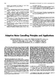
In this section we briefly develop the optimal noise canceller for stationary processes and then extend it to the nonstationary case by embedding it into a Gauss-Markov framework [6,7]. The basic structure of the noise canceller is shown in Fig. 1 where we see that the process is characterized by a space-time signal at the th -sensor of an L-element array in additive white noise as p ( x ; t ) = s ( x ; t ) + η ( x ; t ); = 1, , L , (1) for p, s, η , the respective measurement, signal and noise at position x and time t . We also assume that there exists a reference signal, r ( x ; t ) , correlated to the noise which can be characterized by an invertible impulse response, Hη ( x ; t ) , that is,

r ( x ; t ) = Hη ( x ; t ) ∗η ( x ; t ) .

(2)

Since it is assumed invertible, we can write the primary canceller result [5] that η (x ;t) = H (x ; t) ∗ r(x ; t) (3) for

H ( x ; t ) := Hη−1 ( x ; t ) . The optimal noise cancelling

problem (in terms of this model) is:

Hξ (t , k ) = Cξ (t )Φξ (t , k ) Bξ (k ) for Φξ (t , k ) = Aξ (t − k )

GIVEN the set of discrete space-time sensor measurements, { p( x ; t )} in additive noise, η ( x ; t ) ,

that reduces to

Hξ (t , k ) = Cξ Aξ t −k Bξ for t > k ,

and reference measurements, {r ( x ; t )} correlated to

The solution to this problem is well-known [6-9] and leads to the optimal cancelling (Wiener) filter given by in the stationary case or the adaptive least-mean squared (LMS) solution in the nonstationary case [5,6]. Note that the purpose of the cancelling filter is to “shape” the reference signal such that it best approximates η ( x; t ) , the contaminating noise for removal. Thus, we have that the cancelled output is z ( x ; t ) = p ( x ; t ) − ηˆ ( x ; t ) = s ( x ; t ) + [η ( x ; t ) − ηˆ ( x ; t ) ] (5) = s ( x ; t ) + ⎡⎣η ( x ; t ) − Hˆ ( x ; t ) ∗ r ( x ; t ) ⎤⎦ ≈ s ( x ; t ) Clearly when ηˆ → η , z → s , the desired result is obtained. With this motivation in mind, we construct a Gauss-Markov representation of the canceller that will be used in solving the joint problem. Note that this approach is equivalent to compensating for colored noise [6-8]. Expanding over the Lelements and using the state-space representation, it is easy to show that the noise canceller can be represented (in general) by the Gauss-Markov ship noise model as (see Fig. 1) ξ (t ) = Aξ (t − 1)ξ (t − 1) + Bξ (t − 1) r (t − 1) + wξ (t − 1) , (6)

p(t ) = s(t ) + η(t ) + ν (t ) N ×1

the colored noise state vector and r the with ξ ∈ R ξ known scalar reference noise (input) where the additive zeromean, white gaussian noise sources have respective covariances, Rwξ wξ and Rvξ vξ . Here

p, s, η, ν ∈ C

L×1

are

the respective pressure-field measurement, signal, colored and broadband measurement noise with v ∼N ( 0, Rvv (t ) ) . Aξ ∈ R

Nξ × Nξ

, Bξ ∈ R

Nξ ×1

, Cξ ∈ R

L× Nξ

Signal

s(t )

(4)

η(t ) = Cξ (t )ξ (t ) + vξ (t )

(8)

in the time invariant case. So we see that ship noise can be completely captured by a Gauss-Markov representation in both stationary and nonstationary cases.

the noise η ( x ; t ) for t = 1, , Nt ; FIND the best (minimum error variance) estimate of the noise, ηˆ ( x ; t ) , (or equivalently Hˆ ( x ; t ) ) such that the cancelled output, z ( x ; t ) , is optimal.

H opt = R −rr1ryr

(7)

are the system,

input and measurement matrices corresponding to the ship noise model parameters. Note also that the spatial dimension is now incorporated in the dimensions of the vector-matrices in this model, that is, we have expanded over the L-elements x→x ; = 1, , L which gives in the sensor array, η ( x ; t ) → η(t ); ξ ( x ; t ) → ξ (t ) . Recall that the impulse response of the state-space model is

GAUSS-MARKOV SHIP NOISE MODEL

wξ (t )

Reference

r (t )

Bξ (t )

+

v ξ (t ) −1

ξ (t )

z I

Pressure-Field

Cξ (t )

η(t ) + − +

p(t )

v (t ) Aξ (t )

Fig. 1. Gauss-Markov ship noise model. We assume that the signal can be characterized by a weak target in the far-field of the array given by

s (t ) = α o ei (ωot −k o ⋅x) = α o e (

i ωot − ko sin θo ( xo + vt ) )

,

(9)

for the source parameters: α o , ωo , ko , θ o , xo that are the respective amplitude, temporal frequency, wavenumber, bearing angle and initial sensor location. Since the array is being towed, we include the tow speed, v , as well. We can simplify this model by defining the following terms, s (t ) = α o (t )e −iβo (t ) sin θo ,

(10)

for α o (t ) := α o eiωot and β o (t ) := ko ( xo + vt ) . Note that the statistics are not restricted to be stationary, so we can accommodate the nonstationarities (transients, etc.) that occur naturally in the ocean environment [9]. Using the Gauss-Markov representation of the noise, we can re-define the optimal cancellation problem as: GIVEN a set of discrete noisy pressure-field and reference measurements, {p(t ), r (t )} , t = 1, 2, , Nt in additive noise and the Gauss-Markov model of Eq. (6), FIND the best (minimum variance) estimate of the ship noise, ηˆ (t | t ) , such that the canceller output,

ε p (t ) = p(t ) − ηˆ (t | t ) ≈ s(t ) is optimal. The recursive solution to this problem is given by the MBP (Kalman filter) and shown in Table I (see [6] for details). Under the gaussian assumptions, this provides an optimal estimator for the noise cancellation problem with known signal; however, we must account for the more realistic case of an unknown far-field signal. Next we formulate the underlying joint estimation problem. II. ADAPTIVE MODEL-BASED NOISE CANCELLING

In section we use the models developed in the previous section to develop the adaptive model-based processor (AMBP) for solving the joint cancellation/signal enhancement problem. We show that by augmenting the cancelling filter into the pressure-field representation that the cancelling operation inherently performs the noise cancellation as part of the usual filtering operation. Adaptivity follows by jointly estimating the target and cancelling filter parameters.

⎡ α1 (t )e−ik β1 (t ) sin θ ⎤ ⎡ α eiωt e−ik ( x1 + vt ) sin θ ⎤ ⎥ ⎢ ⎥ ⎢ s(t ) = ⎢ ⎥ ,(11) ⎥=⎢ ⎢ −ik β L (t ) sin θ ⎥ ⎢ iωt −ik ( xL + vt ) sin θ ⎥ ⎣α L (t )e ⎦ ⎣⎢α e e ⎦⎥

For signal enhancement we begin by defining the signal vector in terms of its unknown parameters, s(t ; Θ) , (for a single target), Θ := [α | ω | θ ]′ . In this case we assume that the unknown parameters in the signal model, Θ , are characterized as piecewise constant ( Θ = 0 ) with a discrete Gauss-Markov model given by Θ(t ) = Θ(t − 1) + Δtw Θ (t − 1) ,

(12)

where w Θ ∼ N(0, Rw Θ w Θ ) and Δt is the sampling interval. This parameter vector is then augmented with the cancelling filter by defining the new state vector as ( N + N )×1

x(t ) := [ξ (t ) | Θ(t )]′ ∈ R ξ Θ . The augmented model requires more analysis before we develop the MBP solution. Consider the augmented state-space model first as:

⎡ ξ (t ) ⎤ ⎡ Aξ (t − 1) 0 ⎤ ⎡ ξ (t − 1) ⎤ ⎡ Bξ (t − 1) ⎤ +⎢ ⎥⎢ ⎥ r (t − 1) ⎢Θ(t ) ⎥ = ⎢ Θ(t − 1) ⎥⎦ ⎣ 0 ⎦ I 0 ⎣ ⎦ ⎣ ⎣ ⎦ NOISE ESTIMATOR . (13) ⎡ wξ (t − 1) ⎤ ˆξ (t | t − 1) = A (t − 1)ξˆ (t − 1) + B (t − 1)r (t − 1) [Prediction] ξ ξ +⎢ ⎥ Δtw Θ (t − 1) ⎦ ⎣ ˆ [Predicted Noise] ηˆ (t | t − 1) = Cξ (t )ξ (t | t − 1) Here we note that the cancelling filter and parameters are eη (t ) = η(t ) − ηˆ (t | t − 1) = Cξ (t )ξ (t | t − 1) + vξ (t ) [Innovation] decoupled in the state-space and can therefore be written directly as Reηeη (t )= Cξ (t ) Pξξ (t | t − 1)Cξ′ (t ) + Rvξ vξ (t )[Innov. Covariance] TABLE I OPTIMUM NOISE CANCELLATION

ξˆ (t | t )

= ξˆ (t | t − 1) + Kξ (t )eη (t )

Kξ (t )

= Pξξ (t | t − 1)Cξ′ (t ) Re−1e (t )

[Gain]

ξ (t | t − 1) = ξ (t ) − ξˆ (t | t − 1) CANCELLER ηˆ (t | t ) = C (t )ξˆ (t | t )

[State Est. Error]

η η

ξ

ε p (t )

[Correction]

[Filtered Noise]

= p(t ) − pˆ (t | t ) = p(t ) − ηˆ (t | t ) ≈ s(t )[Cancelled Output]

ξ (t ) = Aξ (t − 1)ξ (t − 1) + Bξ (t − 1)r (t − 1) + wξ (t − 1) Θ(t ) = Θ(t − 1) + Δtw Θ (t − 1)

(14)

Next we note that the pressure-field measurement is the superposition of three distinct components: far-field signal, ship generated noise and instrumentation noise given by p(t ) = s(t ; Θ) signal

+

η(t ) ship noise

+

v (t )

. (15)

measurement noise

where ξ (t | t − 1), Pξξ (t | t − 1) are the state error and covariance. First we note from Eq. (6) that the output of the decoupled cancelling filter remains ( see Eq. (6) )

η(t ) = Cξ (t )ξ (t ) + vξ (t ) . Since s(t ) is assumed to be a far-field source, we have that at the th -sensor, s (t ) = α (t )e −iβ (t ) sin θ . Now expanding over the L -sensor array, we obtain the signal vector

Therefore, substituting into Eq. (15) and accounting for the augmented state vector, we obtain ⎡ ξ (t ) ⎤ p(t ) = ⎡⎣Cξ (t ) | 0 ⎤⎦ ⎢ ⎥ + s(t ; Θ) + vξ (t ) + v (t ) (16) ⎣Θ(t ) ⎦

Since the far-field signal is a nonlinear function of the parameters (augmented states), that is, at the

th

TABLE II JOINT MODEL-BASED PROCESSOR

sensor,

s (t ; Θ) = α (t )e−iβ (t ) = Θ1ei (Θ2t − k ( x + vt ) sin Θ3 for the single target case, then the pressure-field across the array is also a nonlinear function, that is, p(t ) = c [ξ (t ), Θ(t ) ] + v (t ) = ⎡⎣s ( t ; Θ(t ) ) + η(t ) ⎤⎦ + v (t ) = s ( t ; Θ(t ) ) + Cξ (t )ξ (t ) + vξ (t ) + v (t )

EXTENDED KALMAN FILTER

xˆ (t | t − 1) = A ξΘ (t − 1)xˆ (t − 1| t − 1) + BξΘ (t − 1)r (t − 1)[Predict] P(t | t − 1) = A ξΘ [ xˆ ] P(t − 1| t − 1) A ξ′ Θ [ xˆ ] + Rw ξΘ w ξΘ (t − 1) = p(t ) − pˆ (t | t − 1)

ep (t )

(17)

Therefore, we have the following approximate model given by the underlying augmented Gauss-Markov representation as: x(t ) = A ξΘ (t − 1)x(t − 1) + BξΘ (t − 1)r (t − 1) + w ξΘ (t − 1)

[Innov.]

pˆ (t | t − 1) = c [ xˆ (t | t − 1) ] Repep (t ) = CξΘ [ xˆ ] P(t | t − 1)Cξ′ Θ [ xˆ ] + Rvξ vξ (t ) + Rvv (t ) K ξΘ (t )

= P(t | t − 1)C′ξΘ [ xˆ ] Re−1e (t )

xˆ (t | t )

= xˆ (t | t − 1) + K ξΘ (t )ep (t )

P (t | t )

=

∂A ξΘ ∂x x = xˆ

η(t ) = Cξ (t )ξ (t ) + vξ (t )

; CξΘ [ xˆ ] :=

∂c[x] ∂x x = xˆ

If we decompose the state vector and perform the partitioned operations, then we see immediately that the canceling filter and signal parameters are estimated “jointly” along with the enhanced signal and noise estimates as shown in Table III.

⎡ Aξ (t − 1) 0 ⎤ ⎡ Bξ (t − 1) ⎤ where A ξΘ = ⎢ ⎥ , B ξΘ = ⎢ ⎥, I⎦ ⎣ 0 ⎣ 0 ⎦ ⎡ w ξ (t − 1) ⎤ CξΘ = ⎡⎣Cξ (t ) | 0 ⎤⎦ , w ξΘ = ⎢ ⎥ ⎣ w Θ (t − 1) ⎦

and

[Correct]

( I-K ξΘ (t )CξΘ [ xˆ ]) P(t | t − 1)

with jacobians: A ξΘ [ x ] :=

p(t ) = c [ξ (t ), Θ(t ) ] + v (t ) = ⎡⎣s ( t ; Θ(t ) ) + η(t ) ⎤⎦ + v(t )

[Gain]

p p

TABLE III JOINT MODEL-BASED CANCELLER/ENHANCER

PREDICTOR

ξˆ (t | t − 1) = Aξ (t − 1)ξˆ (t − 1| t − 1) + Bξ (t − 1)r (t − 1) ˆ (t | t − 1) = Θ ˆ (t − 1| t − 1) Θ

⎡ Θ eiΘ2t e −ik ( x1 + vt ) sin Θ3 ⎤ ⎢ 1 ⎥ s(t ; Θ) = ⎢ ⎥ ⎢ ⎥ −ik x + vt sin Θ3 ⎢⎣Θ1eiΘ2t e ( L ) ⎥⎦

INNOVATIONS

(18) The basic joint cancelling/signal enhancement problem can now be stated in terms of this augmented Gauss-Markov representation as: GIVEN a set of discrete noisy pressure-field and reference measurements, {p(t ), r (t )} , t = 1, 2, , Nt and the Gauss-Markov model of Eq. (18), FIND the best (minimum variance) estimate of the augmented state (ship noise+signal), xˆ (t | t ) , or equivalently, sˆ (t ; Θ) and ηˆ (t | t ) , such that the canceller output, ε p (t ) = p(t ) − ηˆ (t | t ) is optimal.

ep (t )

ηˆ (t | t − 1) = Cξ (t )ξˆ (t | t − 1) ˆ (t | t − 1) + ηˆ (t | t − 1) pˆ (t | t − 1) = s t ; Θ

(

)

CORRECTOR

ξˆ (t | t )

= ξˆ (t | t − 1) + Kξ (t )ep (t )

ˆ (t | t ) Θ

ˆ (t | t − 1) + K (t )e (t ) =Θ Θ p CANCELLER

ηˆ (t | t )

= Cξ (t )ξˆ (t | t )

ε p (t )

= p(t ) − ηˆ (t | t ) ENHANCER

sˆ (t ; Θ)

We have a linear decoupled state-space, but (unfortunately) a nonlinear measurement system requiring a nonlinear processor. This problem can be solved by a parametrically adaptive MBP using the recursive extended Kalman filter (EKF) given in Table II for the augmented system algorithm.

= p(t )-pˆ (t | t − 1)

(

ˆ (t | t ) = s t; Θ

)

⎡ K ξ (t ) ⎤ (Nξ + N Θ )× N p for K ξΘ (t ) := ⎢ ⎥ with K ξΘ ∈ R ⎣ K Θ (t ) ⎦ and K ξ ∈ R

Nξ × N p

; KΘ ∈ R

NΘ × N p

To formalize the processor further in terms of our ocean acoustic problem, let us first investigate the predicted measurement in more detail to focus on the actual operations performed. We start with the augmented representation, which is a nonlinear function due to the augmentation of the parameters, that is,

(

)

ˆ (t | t − 1) + ηˆ (t | t − 1) pˆ (t | t − 1) = c [ xˆ (t | t − 1) ] = s t ; Θ ˆ ) + C (t )ξˆ (t | t − 1) = s(t ; Θ ξ

,(19)

for ˆ (t|t −1) ⎤ ˆ (t|t −1)t −ik ( x1 + vt ) sin Θ iΘ ⎡Θ 3 ˆ 2 e ⎢ 1 (t | t − 1)e ⎥ ˆ) = ⎢ ⎥ . (20) s(t ; Θ ⎢ ⎥ ˆ (t | t − 1)eiΘˆ 2 (t|t −1)t e−ik ( xL + vt ) sin Θˆ 3 (t|t −1) ⎥ ⎢⎣Θ 1 ⎦

The corresponding innovations for the adaptive processor can also be written in terms of its components as

III. SUMMARY

In this paper we have developed a solution to the joint cancellation/signal enhancement problem using a modelbased approach [6]. Starting with the optimal noise canceller solution we developed the corresponding model-based solution demonstrating their equivalence for the case where the signal is known a priori. Next we developed the solution to the joint problem with the signal unknown, but parameterized as a far-field target. The solution to this problem lead to the parametrically adaptive model-based processor implemented with the (nonlinear) extended Kalman filter (EKF) algorithm. It was shown how to design the processor for this problem. Future efforts will be aimed at applying this technique to both simulated and measured hydrophone data. We plan to use the discrete implementation of the EKF available in MATLAB [10] with the toolbox SSPACK_PC [11].

( )

ˆ − ηˆ (t | t − 1) ep (t ) = p(t ) − pˆ (t | t − 1) = p(t ) − s t ; Θ

(

( ))

ˆ + ( η(t ) − ηˆ (t | t − 1) ) + v (t ) = s(t ) − s t ; Θ

( ) ˆ ) + C (t )ξ (t | t − 1) + v (t ) + v (t ) = s ( t; Θ ξ ξ

ˆ + η(t | t − 1) + v (t ) = s t; Θ

. (21)

[1]

So we see that the joint parametrically adaptive processor is capable of not only providing the optimal cancelling solution ( ηˆ (t | t − 1) → η(t ) ) , but also capable of estimating the far-

(

)

ˆ ) → s(t ) . field target signal for optimal enhancement sˆ (t ; Θ

Using the EKF algorithm it is necessary to provide the jacobians for implementation, that is, ∂a [ξ,Θ ] ∂ξ ∂c [ξ,Θ ] ∂ξ ∂c [ξ,Θ ] ∂ω

= Aξ (t ), = Cξ (t ),

∂a [ξ,Θ ] ∂Θ ∂c [ξ,Θ ] ∂θ

REFERENCES

=I

= iα(t ) β (t ) cos θeiβ (t ) sin θ

∂c [ξ,Θ ] i ωt − β (t ) sin θ ) = itα(t )eiβ (t ) sin θ , =e( ∂α =1, , L

(22) completing the development of the parametrically adaptive solution to the joint cancellation/signal enhancement problem. Next we summarize our results and discuss future efforts.

C. S. Clay and H. Medwin, Acoustical Oceanography, John Wiley, New York, pp. 110-134, 1977. [2] I. Tolstoy and C. S. Clay, Ocean Acoustics: Theory and Experiment in Underwater Sound, Acoust. Soc. Am., New York, pp. 3-12, 1987. [3] W. C. Knight, R. G. Pridham and S. M. Kay. “Digital signal processing for sonar, Proc. IEEE, Vol. 69, (11), pp. 1451-1506, 1981. [4] R. O. Nielsen, Sonar Signal Processing, Artech House, Boston, pp.95-140, 1991. [5] B. Widrow, J. R. Glover, J. M. McCool, et. al., “Adaptive noise cancelling: principles and applications”, Proc. IEEE, Vol. 63, (12), pp. 1692-1716, 1975. [6] J. V. Candy, Model-Based Signal Processing, John Wiley, New York, 2005. [7] A. Jazwinski, Stochastic Processes and Filtering Theory, Academic Press, 1970. [8] B Friedlander, “System Identification techniques for adaptive noise cancelling”, IEEE Trans. Acoust. Speech Signal Proc., Vol. 30, (5), pp. 699-709, 1982. [9] E. J. Sullivan and J. V. Candy, “Space-time array processing: the model-based approach,” J. Acoust. Soc. Am., Vol. 102 (5), Pt. 1, pp. 2809-2820, 1997. [10] Mathworks, MATLAB User’s Manual, Mathworks Inc., Boston, 1993. [11] J. V. Candy and P. M. Candy, “SSPACK_PC: A model-based signal processing package on personal computers,” DSP Applications, Vol. 2 (3), 33-42, 1993.

This work was performed under the auspices of the U.S. Department of Energy by University of California, Lawrence Livermore National Laboratory under contract No. W-7405-Eng-48.