1
Capacity-Achieving Ensembles for the Binary Erasure Channel With Bounded Complexity Henry D. Pfister, Member, Igal Sason, Member, and R¨udiger Urbanke
Abstract We present two sequences of ensembles of non-systematic irregular repeat-accumulate codes which asymptotically (as their block length tends to infinity) achieve capacity on the binary erasure channel with bounded complexity per information bit. This is in contrast to all previous constructions of capacity-achieving sequences of ensembles whose complexity grows at least like the log of the inverse of the gap (in rate) to capacity. The new bounded complexity result is achieved by puncturing bits, and allowing in this way a sufficient number of state nodes in the Tanner graph representing the codes. We derive an information-theoretic lower bound on the decoding complexity of randomly punctured codes on graphs. The bound holds for every memoryless binary-input output-symmetric channel and is refined for the binary erasure channel. Index Terms Binary erasure channel (BEC), codes on graphs, degree distribution (d.d.), density evolution (DE), irregular repeataccumulate (IRA) codes, low-density parity-check (LDPC) codes, memoryless binary-input output-symmetric (MBIOS) channel, message-passing iterative (MPI) decoding, punctured bits, state nodes, Tanner graph.
I. I NTRODUCTION During the last decade, there have been many exciting developments in the construction of low-complexity error-correction codes which closely approach the capacity of many standard communication channels with feasible complexity. These codes are understood to be codes defined on graphs, together with the associated iterative decoding algorithms. By now, there is a large collection of these codes that approach the channel capacity quite closely with moderate complexity. The first capacity-achieving sequences of ensembles of low-density parity-check (LDPC) codes for the binary erasure channel (BEC) were found by Luby et al. [7], [8] and Shokrollahi [17]. Following these pioneering works, Oswald and Shokrollahi presented in [9] a systematic study of capacity-achieving degree distributions (d.d.) for sequences of ensembles of LDPC codes whose transmission takes place over the BEC. Capacity-achieving ensembles of irregular repeat-accumulate (IRA) codes for the BEC were introduced and analyzed in [4], [16], and also capacityachieving ensembles for erasure channels with memory were designed and analyzed in [10], [11]. In [5], [6], Khandekar and McEliece discussed the decoding complexity of capacity-approaching ensembles of irregular LDPC and IRA codes for the BEC and more general channels. They conjectured that if the achievable rate under message-passing iterative (MPI) decoding is a fraction 1 − ε of the channel capacity with vanishing bit error (or erasure) probability, then for a wide class of channels, the decoding complexity scales like 1ε ln 1ε . This conjecture is based on the assumption that the number of edges (per information bit) in the associated bipartite graph scales like ln 1ε , and the required number of iterations under MPI decoding scales like 1ε . There is one exception for capacity-achieving and low-complexity ensembles of codes on the BEC, where the decoding complexity under the MPI algorithm behaves like ln 1ε (see [7], [15], [16], [17]). This is true since the absolute reliability provided by the BEC allows every edge in the graph to be used only once during MPI decoding. The paper was published in the IEEE Trans. on Information Theory, vol. 51, no. 7, pp. 2352–2379, July 2005. It was submitted in August 25, 2004 and revised in December 5, 2004. This work was presented in part at the 23rd IEEE Convention of Electrical & Electronics Engineers in Israel, September 2004, and at the 42nd Annual Allerton Conference on Communication, Control and Computing, IL, USA, October 2004. Communicated by Robert McEliece, Associate Editor for Coding Theory. Henry D. Pfister was with Qualcomm, Inc. in San Diego, CA., USA when the work was done. He is now with EPFL – Swiss Federal Institute of Technology, Lausanne, CH–1015, Switzerland (e-mail:
[email protected]). Igal Sason is with the Department of Electrical Engineering, Technion–Israel Institute of Technology, Haifa 32000, Israel (e-mail:
[email protected]). R¨udiger Urbanke is with EPFL – Swiss Federal Institute of Technology, Lausanne, CH–1015, Switzerland (e-mail:
[email protected]).
2
In [15], Sason and Urbanke considered the question of how sparse can parity-check matrices of binary linear codes be, as a function of their gap (in rate) to capacity (where this gap depends on the channel and the decoding algorithm). If the code is represented by a standard Tanner graph without state nodes, the decoding complexity per iteration under MPI decoding is strongly linked to the density of the corresponding parity-check matrix (i.e., the number of edges in the graph per information bit). In particular, they considered an arbitrary sequence of binary linear codes which achieves a fraction 1 − ε of the capacity of a memoryless binary-input output-symmetric (MBIOS) channel with vanishing bit error probability. By information-theoretic tools, they proved that for every such sequence of codes and every sequence of parity-check matrices which represent these codes, the asymptotic K1 +K2 ln 1ε density of the parity-check matrices grows at least like where K1 and K2 are constants which were 1−ε given explicitly as a function of the channel statistics (see [15, Theorem 2.1]). It is important to mention that this bound is valid under ML decoding, and hence, it also holds for every sub-optimal decoding algorithm. The tightness of the lower bound for MPI decoding on the BEC was demonstrated in [15, Theorem 2.3] by analyzing the capacity-achieving sequence of check-regular LDPC-code ensembles introduced by Shokrollahi [17]. Based on the discussion in [15], it follows that for every iterative decoder which is based on the standard Tanner graph, there exists a fundamental tradeoff between performance and complexity, and the complexity (per information bit) becomes unbounded when the gap between the achievable rate and the channel capacity vanishes. Therefore, it was suggested in [15] to study if better performance versus complexity tradeoffs can be achieved by allowing more complicated graphical models (e.g., graphs which also involve state nodes). In this paper, we present sequences of capacity-achieving ensembles for the BEC with bounded encoding and decoding complexity per information bit. Our framework therefore yields practical encoding and decoding algorithms that require linear time, where the constant factor which is implied by the linear time is independent of ε (and is in fact quite small). The new ensembles are non-systematic IRA codes with properly chosen d.d. (for background on IRA codes, see [4] and Section II). The new bounded complexity results under MPI decoding improve on the results in [16], and demonstrate the superiority of properly designed non-systematic IRA codes over systematic IRA codes (since with probability 1, the complexity of any sequence of ensembles of systematic IRA codes grows at least like ln 1ε , and hence, it becomes unbounded under MPI decoding when the gap between the achievable rate and the capacity vanishes (see [16, Theorem 1])). The new bounded complexity result is achieved by allowing a sufficient number of state nodes in the Tanner graph representing the codes. Hence, it answers in the affirmative a fundamental question which was posed in [15] regarding the impact of state nodes in the graph on the performance versus complexity tradeoff under MPI decoding. We suggest a particular sequence of capacity-achieving ensembles of non-systematic IRA codes where the degree of the parity-check nodes is 5, so the complexity per information 5 when the gap (in rate) to capacity vanishes (p designates the bit erasure bit under MPI decoding is equal to 1−p probability of the BEC). We note that our method of truncating the check d.d. is similar to the bi-regular check d.d. introduced in [19] for non-systematic IRA codes. Simulations results which are presented in this paper to validate the claims of our theorems, compare our new ensembles with another previously known ensemble. This is meant to give the reader some sense of their relative performance. We note that for fixed complexity, the new codes eventually (for n large enough) outperform any code proposed to date. On the other hand, the convergence speed to the ultimate performance limit is expected to be quite slow, so that for moderate lengths, the new codes are not expected to be record breaking. It is important to note that we do not claim optimality of our ensembles, but the main point here is showing for the first time the existence of IRA codes in which their encoding and decoding complexity per information bit remain bounded as the code threshold approaches the channel capacity. We also derive in this paper an information-theoretic lower bound on the decoding complexity of randomly punctured codes on graphs. The bound holds for every MBIOS channel with a refinement for the particular case of a BEC. The structure of the paper is as follows: Section II provides preliminary material on ensembles of IRA codes, Section III presents our main results which are proved in Section IV. Analytical and numerical results for the considered degree distributions and their asymptotic behavior are discussed in Section V. Practical considerations and simulation results for our ensembles of IRA codes are presented in Section VI. We conclude our discussion in Section VII. Three appendices also present important mathematical details which are related to Sections IV and V.
3
II. IRA C ODES We consider here ensembles of non-systematic IRA codes. We assume that all information bits are punctured. The Tanner graph of these codes is shown in Fig. 1. These codes can be viewed as serially concatenated codes where the encoding process is done as follows: the outer code is a mixture of repetition codes of varying order, the bits at the output of the outer code are interleaved, and then partitioned into disjoint sets (whose size is not fixed in general). The parity of each set of bits is computed, and then these bits are accumulated (so the inner code is a differential encoder). DE
information bits
x0
x3
x1
x2
random permutation
parity checks code bits
Fig. 1.
The Tanner graph of IRA codes.
Using P standard notation, an ensemble codes is characterized by its block length n and its d.d. pair P∞ of IRA ∞ i−1 and ρ(x) = i−1 . Here, λ (or ρ , respectively) designates the probability that a λ(x) = λ x ρ x i i i=1 i i=1 i randomly chosen edge, among the edges that connect the information nodes and the parity-check nodes, is connected to an information bit node (or to a parity-check node) of degree i. As is shown in Fig. 1, every parity-check node is also connected to two code bits; this is a consequence ofP the differential encoder which is the inner code of these i serially concatenated and interleaved codes. Let R(x) = ∞ i=1 Ri x be a power series where the coefficient Ri denotes the fraction of parity-check nodes that are connected to i information nodes. Then it is easy to show that iRi ρi = P∞ j=1 jRj
or equivalently Ri =
ρi P∞i ρj j=1 j
which yields that the polynomials R(·) and ρ(·) are related by the equation Rx ρ(t) dt . R(x) = R01 0 ρ(t) dt
(1)
We assume that the permutation in Fig. 1 is chosen uniformly at random from the set of all permutations. The transmission of a randomly selected code from this ensemble takes place over a BEC with erasure probability p. The asymptotic performance of the MPI decoder (as the block length tends to infinity) can be analyzed by tracking the average fraction of erasure messages which are passed in the graph of Fig. 1 during the lth iteration. This technique was introduced in [13] and is known as density evolution (DE). In the asymptotic case where the block length tends to infinity, the messages which are passed through the edges of the Tanner graph are statistically independent, so the cycle-free condition does indeed hold for IRA codes. A single iteration first includes the update of the messages in the Tanner graph from the code nodes to the parity-check nodes, then the update of the messages from the parity-check nodes to the information nodes, and (l) vice versa. Using the same notation as in [4], let x0 be the probability of erasure for a message from information (l) (l) nodes to parity-check nodes, x1 be the probability of erasure from parity-check nodes to code nodes, x2 be the (l) probability of erasure from code nodes to parity-check nodes, and finally, let x3 be the probability of erasure for messages from parity-check nodes to information nodes (see Fig. 1). From the Tanner graph of IRA codes in Fig. 1, an outgoing message from a parity-check node to a code node is not an erasure if and only if all the incoming messages at the same iteration from the information nodes to the parity-check nodes are not erasures, and also the incoming message through the other edge which connects a code node to the same parity-check node is not an erasure either. Since a fraction Ri of the parity-check nodes are of degree i (excluding the two edges which connect every parity-check node to two code nodes), then the average probability that at the lth iteration, all the incoming messages through the edges from the information nodes to an arbitrary parity-check node in the graph
4
P (l) i (l) are not erasures is equal to ∞ i=1 Ri (1 − x0 ) = R(1 − x0 ). Following the cycle-free concept which is valid for the asymptotic case where the block length tends to infinity, we obtain that (l)
(l)
(l)
1 − x1 = (1 − x2 ) R(1 − x0 ).
It is also clear from Fig. 1 that the outgoing message from a parity-check node to an information node is not an erasure if and only if the incoming messages through the other edges which connect this parity-check node to information nodes in the graph are not erasures, and also the incoming messages through the two edges which connect this parity-check node to code nodes are not erasures either. The number of bits involved in short cycles become negligible as n gets large. DE assumes all messages are statistically independent in the asymptotic case, and the concentration theorem justifies this assumption. Hence, for an arbitrary edge which is connected to a parity-check node, the average probability that all the incoming messages through the other edges connecting this parity-check node are not erasures is equal to ∞ X i=1
(l)
(l)
ρi (1 − x0 )i−1 = ρ(1 − x0 ).
The probability that the two incoming messages passed at iteration l from two consecutive code nodes to the (l) parity-check node which is connected to them are both not erasures is equal to (1 − x2 )2 , so we obtain that (l)
(l)
(l)
1 − x3 = (1 − x2 )2 ρ(1 − x0 ).
For variable nodes in the Tanner graph, the outgoing message will be an erasure if and only if all the incoming messages through the other edges connecting this node are erasures and also the information we get about this node from the BEC is an erasure too. The update rule of the messages at the information nodes in Fig. 1 therefore (l) (l) implies that x0 = λ(x3 ), and this follows since we assume here that all the information nodes are punctured (hence, there is no information about the values of the information bits which comes directly from the BEC). Since all the code bits in the Tanner graph of Fig. 1 are transmitted over the BEC, then the update rule of the messages (l) (l−1) at the code bits implies that x2 = px1 . We now assume that we are at a fixed point of the MPI decoding algorithm, and solve for x0 . From the last four equalities, we obtain the following equations: x1 = 1 − (1 − x2 ) R(1 − x0 ) x2 = px1
2
x3 = 1 − (1 − x2 ) ρ(1 − x0 ) x0 = λ(x3 ).
(2) (3) (4) (5)
The only difference between (2)–(5) and the parallel equations in [4] is the absence of a factor p in the RHS of (5). This modification stems from the fact that all information bits are punctured in the ensemble considered. Solving this set of equations for a fixed point of iterative decoding provides the equation à ! · ¸2 1−p x0 = λ 1 − ρ(1 − x0 ) . (6) 1 − pR(1 − x0 ) If Eq. (6) has no solution in the interval (0, 1], then according to the DE analysis of MPI decoding, the bit erasure probability must converge to zero. Therefore, the condition that à ! · ¸2 1−p λ 1− ρ(1 − x) < x, ∀x ∈ (0, 1] (7) 1 − pR(1 − x) implies that MPI decoding obtains a vanishing bit erasure probability as the block length tends to infinity. The design rate of the ensemble of non-systematic IRA codes can be computed by matching edges in the Tanner graph shown in Fig. 1. In particular, the number of edges in the permutation must be equal to both the number of
5
information bits times the average information bit degree and the number of code bits times the average parity-check degree. This implies that the design rate of non-systematic IRA ensembles is equal to R1 λ(x) dx IRA R = R01 . (8) ρ(x) dx 0
Furthermore, we will see later that RIRA = 1 − p for any pair of d.d. (λ, ρ) which satisfies Eq. (6) for all x0 ∈ [0, 1] (see Lemma 1 in Section IV). In order to find a capacity-achieving ensemble of IRA codes, we generally start by finding a d.d. pair (λ, ρ) with non-negative power series expansions which satisfies Eq. (6) for all x0 ∈ [0, 1]. Next, we slightly modify λ(·) or ρ(·) so that Eq. (7) is satisfied and the new design rate in Eq. (8) is equal to (1 − ε)(1 − p) for an arbitrarily small ε > 0. Since the capacity of the BEC is 1 − p, this gives an ensemble which has vanishing bit erasure probability under MPI decoding at rates which are arbitrarily close to capacity. III. M AIN R ESULTS Definition 1: [Capacity-Approaching Codes] Let {Cm } be a sequence of binary linear codes of rate Rm , and assume that for every m, the codewords of the code Cm are transmitted with equal probability over a channel whose capacity is C . This sequence is said to achieve a fraction 1 − ε of the channel capacity with vanishing bit error probability if limm→∞ Rm ≥ (1 − ε)C , and there exists a decoding algorithm under which the average bit error probability of the code Cm tends to zero in the limit where m tends to infinity.1 Definition 2: [Encoding and Decoding Complexity] Let C be an ensemble of IRA codes with a d.d. pair λ(·) and ρ(·). Suppose the transmission takes place over a BEC, and the ensemble achieves a fraction 1 − ε of the channel capacity with vanishing bit erasure probability. The encoding and the decoding complexity are measured in operations per information bit, and under MPI decoding, they are defined as the number of edges per information bit in the Tanner graph. We denote the asymptotic encoding and decoding complexity by χE (ε, C) and χD (ε, C), respectively (note that as the block length of the codes tends to infinity, the complexity of a typical code from this ensemble concentrates around the average complexity). Theorem 1: [Capacity-Achieving Bit-Regular Ensembles for the BEC with Bounded Complexity] Consider the ensemble of bit-regular non-systematic IRA codes C , where the d.d. of the information bits is given by λ(x) = xq−1 ,
q≥3
(9)
which implies that each information bit is repeated q times. Assume that the transmission takes place over a BEC with erasure probability p, and let the d.d. of the parity-check nodes2 be 1
1 − (1 − x) q−1 ρ(x) = " # . µ i¶ 2 h q 1 − p 1 − qx + (q − 1) 1 − (1 − x) q−1
(10)
Let ρn be the coefficient of xn−1 in the power series expansion of ρ(x) and, for an arbitrary ² ∈ (0, 1), define M (ε) to be the smallest positive integer3 M such that M X
n=2
ρn > 1 −
ε . q(1 − p)
The ε-truncated d.d. of the parity-check nodes is given by M (ε) M (ε) X X ρn xn−1 . ρn + ρε (x) = 1 − n=2
1
(11)
(12)
n=2
We refer to vanishing bit erasure probability for the particular case of a BEC. The d.d. of the parity-check nodes refers only to the connection of the parity-check nodes with the information nodes. Every parity-check node is also connected to two code bits (see Fig. 1), but this is not included in ρ(x). P∞ PM 3 The existence of M (ε) for ε ∈ (0, 1) follows from the fact that ρn = O(n−q/(q−1) ¡ 1 ) ¢and n=2 ρn = 1. This implies that n=2 ρn can be made arbitrarily close to 1 by increasing M . It can be shown that M (ε) = O εq−1 . 2
6 1 ], the polynomial ρε (·) has only non-negative coefficients, and the d.d. pair (λ, ρε ) achieves For q = 3 and p ∈ (0, 13 a fraction 1 − ε of the channel capacity with vanishing bit erasure probability under MPI decoding. Moreover, the complexity (per information bit) of encoding and decoding satisfies
χE (ε, C) = χD (ε, C) < q +
2 . (1 − p)(1 − ε)
(13)
2 . In the limit where ε tends to zero, the capacity is achieved with a bounded complexity of q + 1−p Theorem 2: [Capacity-Achieving Check-Regular Ensembles for the BEC with Bounded Complexity] Consider the ensemble of check-regular non-systematic IRA codes C , where the d.d. of the parity-check nodes is given by ρ(x) = x2 . (14)
Assume that the transmission takes place over a BEC with erasure probability p, and let the d.d. of the information bit nodes be4 Ãr à !! λ(x) = 1 +
2p(1 − x)2 sin √
1 3
3 (1 −
arcsin
p)4
− 27p(1−x) 4(1−p)3
¶3 µ 3 2 p(1−x) 2 − (1−p)3
3 2
.
(15)
Let λn be the coefficient of xn−1 in the power series expansion of λ(x) and, for an arbitrary ² ∈ (0, 1), define M (ε) to be the smallest positive integer5 M such that M X λn
n=2
n
>
(1 − p)(1 − ε) . 3
(16)
This infinite bit d.d. is truncated by treating all information bits with degree greater than M (ε) as pilot bits (i.e., these information bits are set to zero). Let λε (x) be the ε-truncated d.d. of the bit nodes. Then, for all p ∈ [0, 0.95], the polynomial λε (·) has only non-negative coefficients, and the modified d.d. pair (λε , ρ) achieves a fraction 1 − ε of the channel capacity with vanishing bit erasure probability under MPI decoding. Moreover, the complexity (per information bit) of encoding and decoding is bounded and satisfies χE (ε, C) = χD (ε, C)
0 can be made arbitrarily small. This proof requires though to verify the positivity of a fixed number of the d.d. coefficients, where this number grows considerably as ε tends to zero. We chose to verify it for all n ∈ N and p ∈ [0, 0.95]. We note that a direct numerical calculation of {λn } for small to moderate values of n, and the asymptotic behavior of λn (which is derived in Appendix B) strongly supports Conjecture 2. Theorem 3: [An Information-Theoretic Bound on the Complexity of Punctured Codes over the BEC] Let 0 } be a sequence of binary linear block codes, and let {C } be a sequence of codes which is constructed {Cm m 0 }.6 Let P by randomly puncturing information bits from the codes in {Cm pct designate the puncturing rate of the information bits, and suppose that the communication of the punctured codes takes place over a BEC with erasure probability p, and that the sequence {Cm } achieves a fraction 1−ε of the channel capacity with vanishing bit erasure probability. Then with probability 1 w.r.t. the random puncturing patterns, and for an arbitrary representation of the 0 } by Tanner graphs, the asymptotic decoding complexity under MPI decoding satisfies sequence of codes {Cm ¡ ¢ p ln Pεeff ´ + lmin ³ lim inf χD (Cm ) ≥ (19) m→∞ 1 1 − p ln 1−Peff where
Peff , 1 − (1 − Ppct )(1 − p)
(20)
and lmin designates the minimum number of edges which connect a parity-check node with the nodes of the parity bits.7 Hence, a necessary condition for a sequence of randomly punctured codes {Cm } to achieve the capacity of the BEC with bounded complexity is that the puncturing rate of the information bits satisfies the condition Ppct = 1 − O(ε). Theorem 4 suggests an extension of Theorem 3, though as will be clarified later, the lower bound in Theorem 3 is at least twice larger than the lower bound in Theorem 4 when applied to the BEC. Theorem 4: [An Information-Theoretic Bound on the Complexity of Punctured Codes: General Case] Let 0 } be a sequence of binary linear block codes, and let {C } be a sequence of codes which is constructed {Cm m 0 }. Let P by randomly puncturing information bits from the codes in {Cm pct designate the puncturing rate of the information bits, and suppose that the communication takes place over an MBIOS channel whose capacity is equal to C bits per channel use. Assume that the sequence of punctured codes {Cm } achieves a fraction 1 − ε of the channel capacity with vanishing bit error probability. Then with probability 1 w.r.t. the random puncturing patterns, 0 } by Tanner graphs, the asymptotic decoding and for an arbitrary representation of the sequence of codes {Cm complexity per iteration under MPI decoding satisfies ³ ´ 1 1−(1−Ppct )C ln ε 2C ln 2 1−C ´ ³ (21) lim inf χD (Cm ) ≥ m→∞ 1 2C ln (1−Ppct )(1−2w)
where
w,
1 2
Z
+∞
min (f (y), f (−y)) dy
(22)
−∞
and f (y) , p(y|x = 1) designates the conditional pdf of the channel, given the input is x = 1. Hence, a necessary condition for a sequence of randomly punctured codes {Cm } to achieve the capacity of an MBIOS channel with bounded complexity per iteration under MPI decoding is that the puncturing rate of the information bits satisfies Ppct = 1 − O(ε). Remark 1 (Deterministic Puncturing): It is worth noting that Theorems 3 and 4 both depend on the assumption that the set of information bits to be punctured is chosen randomly. It is an interesting open problem to derive 6 0 Since we do not require that the sequence of original codes {Cm } is represented in a systematic form, then by saying ’information bits’, 0 we just refer to any set of bits in the code Cm whose size is equal to the dimension of the code and whose corresponding columns in 0 the parity-check matrix are linearly independent. If the sequence of the original codes {Cm } is systematic (e.g., turbo or IRA codes before puncturing), then it is natural to define the information bits as the systematic bits of the code. 7 The fact that the value of lmin can be changed according to the choice of the information bits is a consequence of the bounding technique.
8
information-theoretic bounds that apply to every puncturing pattern (including the best carefully designed puncturing pattern for a particular code). We also note that for any deterministic puncturing pattern which causes each paritycheck to involve at least one punctured bit, the bounding technique which is used in the proofs of Theorems 3 and 4 becomes trivial and does not provide a meaningful lower bound on the complexity in terms of the gap (in rate) to capacity. IV. P ROOF
OF THE
M AIN T HEOREMS
In this section, we prove our main theorems. The first two theorems are similar and both prove that under MPI decoding, specific sequences of ensembles of non-systematic IRA codes achieve the capacity of the BEC with bounded complexity (per information bit). The last two theorems provide an information-theoretic lower bound on the decoding complexity of randomly punctured codes on graphs. The bound holds for every MBIOS channel and is refined for a BEC. The approach used in the first two theorems was pioneered in [7] and can be broken into roughly three steps. The first step is to find a (possibly parameterized) d.d. pair (λ, ρ) which satisfies the DE equation (6). The second step involves constructing an infinite set of parameterized (e.g., truncated or perturbed) d.d. pairs which satisfy inequality (7). The third step is to verify that all of coefficients of the d.d. pair (λ, ρ) are non-negative and sum to one for the parameter values of interest. Finally, if the design rate of the ensemble approaches 1 − p for some limit point of the parameter set, then the ensemble achieves the channel capacity with vanishing bit erasure probability. The following lemma simplifies the proof of Theorems 1 and 2. Its proof is based on the analysis of capacityachieving sequences for the BEC in [17], and the extension to erasure channels with memory in [10], [11]. Lemma 1: Any pair of d.d. functions (λ, ρ) which satisfy λ(0) = 0, λ(1) = 1, and satisfy the DE equation (6) for all x0 ∈ [0, 1] also have a design rate (8) of 1 − p (i.e., it achieves the capacity of a BEC whose erasure probability is p). Proof: We start with Eq. (6) and proceed by substituting x0 = 1 − x, applying λ−1 (·) to both sides, and moving things around to get µ ¶2 1−p −1 1 − λ (1 − x) = ρ(x). (23) 1 − pR(x) Integrating both sides from x = 0 to x = 1 gives ¶2 Z 1µ Z 1 ¡ ¢ 1−p −1 1 − λ (1 − x) dx = ρ(x) dx. 1 − pR(x) 0 0 Since λ(·) is positive, monotonic increasing and λ(0) = 0, λ(1) = 1, we can use the identity Z 1 Z 1 λ−1 (x) dx = 1 λ(x) dx +
to show that
(24)
0
0
¶2 1−p ρ(x) dx. 1 − pR(x) 0 0 Taking the derivative of both sides of Eq. (1) shows that Z 1 ρ(x) = ρ(x) dx · R0 (x) Z
1
λ(x) dx =
Z
1µ
0
and then it follows easily that Z 1 0
¶2 1−p ρ(x) dx · λ(x)dx = R0 (x)dx 1 − pR(x) 0 0 ¶ Z R(1) µ Z 1 1−p 2 du ρ(x) dx · = 1 − pu R(0) 0 Z 1 ρ(x) dx = (1 − p) · Z
1
Z
1µ
0
where the fact that R(0) = 0 and R(1) = 1 is implied by Eq. (1). Dividing both sides by the integral of ρ(·) and using Eq. (8) shows that the design rate RIRA = 1 − p.
9
A. Proof of Theorem 1 1) Finding the D.D. Pair: Consider a bit-regular ensemble of non-systematic IRA codes whose d.d. pair (λ, ρ) satisfies the DE equation (6). We approach the problem of finding the d.d. pair by solving Eq. (6) for ρ(·) in terms of λ(·) and the progression is actually similar to the proof of Lemma 1, except that the limits of integration change. Starting with Eq. (23) and integrating both sides from x = 0 to x = t gives Z t ¡ ¢ 1 − λ−1 (1 − x) dx 0 ¶2 Z tµ 1−p = ρ(x) dx 1 − pR(x) 0 ¶2 0 Z tµ 1−p R (x) = dx 1 − pR(x) R0 (1) 0 (1 − p)2 R(t) = (25) R0 (1) 1 − pR(t)
where the substitution ρ(x) = R0 (x)/R0 (1) follows from Eq. (1). The free parameter R0 (1) can be determined by requiring that the d.d. R(·) satisfy R(1) = 1. Solving Eq. (25) for R0 (1) with t = 1 and R(1) = 1 shows that R0 (1) = R 1 0
1−p
(1 − λ−1 (1 − x)) dx
.
(26)
Solving Eq. (25) for R(t) and substituting for R0 (1) gives R(t) = 1−p
For simplicity, we now define Q(x) ,
substitute x for t, and get
Rt (1−λ−1 (1−x)) dx R 01 (1−λ−1 (1−x)) dx 0 Rt (1−λ−1 (1−x)) dx + p · R 01 (1−λ−1 (1−x)) dx 0
Rx¡
1 − λ−1 (1 − t) R01 −1 0 (1 − λ (1 − t))
R(x) =
It follows from Eqs. (1) and (28) that ρ(x) = = = =
and
¢
.
dt dt
Q(x) . 1 − p + pQ(x)
R0 (x) R0 (1) (1 − p)Q0 (x) (1 − p + pQ(1))2 (1 − p + pQ(x))2 (1 − p)Q0 (1) 1 Q0 (x) (1 − p + pQ(x))2 Q0 (1) 1 − λ−1 (1 − x) (1 − p + pQ(x))2
ρ(1) =
1 − λ−1 (0) = 1. (1 − p + pQ(1))2
(27)
(28)
(29)
(30)
The important part of this result is that there is no need to truncate the power series of ρ(·) to force ρ(1) = 1. This appears to be an important element of ensembles with bounded complexity. Now, consider the bit-regular case where every information bit is repeated q ≥ 3 times (i.e., λ(x) = xq−1 ). From Eq. (27), it can be verified with some algebra that i h q (31) Q(x) = qx − (q − 1) 1 − (1 − x) q−1 .
10
Substituting this into Eq. (29) gives the result in Eq. (10). Finally, we show that the power series expansion of Eq. (10) defines a proper probability distribution. First, we 1 note that p ∈ (0, 13 ] by hypothesis, and that Appendix A establishes the non-negativity of the d.d. coefficients {ρn } under this same condition. Since ρ(1) = 1, these coefficients must sum to one if the power series expansion converges at x = 1. This follows from the asymptotic expansion, given later in (63), which implies that ρn = O(n−q/(q−1) ). Therefore, the function ρ(x) defines a proper d.d. 2) Truncating the D.D.: Starting with the d.d. pair (λ,ρ) implied by Eq. (29) (which yields that Eq. (6) holds), we apply Lemma 1 to show that the design rate is 1 − p. The next step is to slightly modify the check d.d. so that the inequality (7) is satisfied instead. In particular, one can modify the ρ(x) from (29) so that the resulting ensemble of bit-regular non-systematic IRA codes is equal to a fraction 1 − ε of the BEC capacity. Let us define M (ε) to be the smallest positive integer M such that the condition in (11) is satisfied. Such an M exists for any ε ∈ (0, 1) because ρn = O(n−q/(q−1) ). We define the ε-truncation of ρ(·) to be the new check degree polynomial in (12), which is also equal to M (ε) ∞ X X ρi + ρi xi−1 (32) ρε (x) = ρ1 + i=2
i=M (ε)+1
and satisfies ρε (1) = ρ(1) = 1. Based on Eqs. (11) and (32), and since the power series expansion of ρ(·) is non-negative for small enough values of p (see Appendix A), then for these values of p Z 1 Z 1 ∞ X ρi ρ(x) dx + ρε (x) dx < 0
0
< =
Z
i=M (ε)+1
1
ρ(x) dx + 0
1+ε . q(1 − p)
ε q(1 − p)
Applying Eq. (8) to the last equation, shows that the design rate of the new ensemble (λ, ρε ) of bit-regular, non-systematic IRA codes is given by R1 λ(x) dx 1 1−p IRA R = R 01 . = R1 > 1+ε q 0 ρε (x) dx 0 ρε (x) dx Using the fact that
1 1+ε
> 1 − ε, for ε > 0, we get the final lower bound RIRA > (1 − p) (1 − ε).
(33)
This shows that the design rate of the new ensemble of codes is equal at least to a fraction 1 − ε of the capacity of the BEC. Now, we need to show that the new ensemble satisfies the inequality (7), which is required for successful decoding, given by à ! · ¸2 1−p λ 1− ρε (1 − x) < x, ∀x ∈ (0, 1] (34) 1 − p Rε (1 − x) where Rε (·) can be computed from ρε (·) via Eq. (1). Since the truncation of ρ(x) only moves edges from high degree checks (i.e., xj terms with j > M ) to degree one checks (i.e. the x0 term), it follows that ρε (x) > ρ(x) ,
∀x ∈ [0, 1).
(35)
Rε (x) > R(x) ,
∀x ∈ (0, 1).
(36)
We will also show that Lemma 2:
11
Proof: We rely on Eqs. (1), (10) and (32) to show that for an arbitrary ε > 0 P ρ1 + ∞ i=M (ε)+1 ρi Rε (x) = ·x P∞ PM (ε) ρ1 + i=M (ε)+1 ρi + i=2 ρii PM (ε) ρi i i=2 i · x + P∞ PM (ε) ρi ρ1 + i=M (ε)+1 ρi + i=2 i ∞ X (ε) Ri xi ,
(37)
i=1
and
R(x) =
ρ1 ρ1 + +
,
ρ1 ∞ X
·x
PM (ε) ρi ρi i=M (ε)+1 i + i=2 i P∞ ρi i i=2 i · x P∞ PM (ε) ρi ρi i=M (ε)+1 i + i=2 i
P∞
+
Ri xi .
(38)
i=1
It is easy to verify that the coefficients in the power series expansions of Rε (·) and R(·) in (37) and (38), respectively, are all non-negative and each of them sum to one. By comparing the two, it follows easily that (ε)
Ri
Since
P∞
i=1 Ri
=
(ε) i=1 Ri
P∞
< Ri
∀ i ≥ 2.
= 1, then (ε)
R1 > R1 .
Let
(ε)
δ i , Ri − R i i = 1, 2, . . . P∞ P∞ P∞ P (ε) then δ1 = − i=2 δi (since by definition, i=1 δi = i=1 Ri − ∞ = 0), and δi > 0 for every integer i=1 Ri i ≥ 2. It therefore follows that for x ∈ (0, 1) R(x) − Rε (x) = δ1 x +
∞ X i=2
i
δ i x < δ1 x +
∞ X
δi x = 0
i=2
which proves the inequality in (36). The validity of the condition in (34) follows immediately from the two inequalities in (35) and (36), and the fact that the d.d. pair (λ, ρ) satisfies the equality in (6) for all x0 ∈ [0, 1]. B. Proof of Theorem 2 1) Finding the D.D. Pair: Like in the proof of Theorem 1, we start the analysis by solving equation (6), but this time we calculate λ(·) for a particular choice of ρ(·). Let us choose ρ(x) = x2 , so R(x) = x3 , and we obtain from the equivalent equation in (23) that the inverse function of λ(·) is equal to µ ¶2 1−p −1 λ (x) = 1 − (1 − x)2 . (39) 1 − p(1 − x)3
Inserting (39) into (15) shows that the expression of λ(·) in (15) is the inverse function to (39) for x ∈ [0, 1], so (15) gives us a closed form expression of λ(·) in the interval [0, 1]. As we noted already, for real numbers, one can simplify the expression of λ(·) in (15), but since we consider it later as a function of a complex argument, then we prefer to leave it in the form of (15).
12
In the following, we show how (15) was derived. Note that since we already verified the correctness of (15), then in the following derivation we do not need to worry about issues of convergence. Set √ 1−y −1 y = λ (x) , z = , u = 1 − x. 1−p With this notation and for u ∈ [0, 1], (39) can be written in the form zφ(u) = u
where φ(u) = 1 − pu3 . We now use the Lagrange inversion formula (see, e.g., [1, Section 2.2]) to obtain the power series expansion of u = u(z) around z = 0, i.e., we write ∞ X uk z k . u(z) = k=0
If z = 0 then u = 0, so u0 = u(0) = 0. The Lagrange inversion formula states that 1 uk = [uk−1 ] φk (u), k = 1, 2, . . . (40) k where [uk−1 ] φk (u) is the coefficient of uk−1 in the power series expansion of φk (u). From the definition of φ(·), the binomial formula gives ¾ µ ¶ k ½ X j 3j k 3 k j k p u φ (u) = (1 − pu ) = (−1) (41) j j=0
so from (40) and (41)
uk =
We conclude that
(−1) k
k−1 3
¡
u(z) = k:
k
k−1 3
0
X
¢
k−1 ∈N 3
p
k−1 3
, if k = 1, 4, 7, 10, . . .
.
otherwise (
(−1) k
k−1 3
µ
k k−1 3
p
k−1 3
zk
)
√
1−y where N designates the set of non-negative integer numbers. Since z = 1−p , then we get ) ( ¶ k−1 k−1 µ X k p 3 (−1) 3 k (1 − y) 2 u= k−1 k (1 − p)k 3 k−1 k:
3
∈N
and x = 1 − u = λ(y) (since y = λ−1 (x)). Finally, we obtain a power series expansion for λ(·) from the last two equalities ) ( ¶ k−1 k−1 µ X k p 3 k (−1) 3 λ(x) = 1 − · (1 − x) 2 . k−1 k (1 − p)k 3 k−1 k:
3
∈N
By substituting k = 3l + 1 where l ∈ N, the latter equation can be written as ¶ µ ¾ ∞ ½ 1 X (−1)l 3l + 1 3l+1 t λ(x) = 1 − √ 3 p l 3l + 1 l=0 ³√ ´ √ 3 p where t , 1−p 1 − x. Fortunately, the final sum can be expressed in closed form and leads to the expression of λ(·) in (15). Plots of the function λ(·) as a function of p ∈ (0, 1) are depicted in Fig. 2. Finally, we show that the power series expansion of Eq. (15) defines a proper probability distribution. Three different representations of the d.d. coefficients {λn } are presented in Section V-B.1 and derived in Appendix B. They are also used in Appendix C to prove the non-negativity of the d.d. for p ∈ [0, 0.95]. Since λ(1) = 1, these coefficients must also sum to one if the power series expansion converges at x = 1. The fact that λn = O(n−3/2 ) follows from a later discussion (in Section V-B.2) and establishes the power series convergence at x = 1. Therefore, the function λ(x) gives a well-defined d.d.
13 1 λ(x) for p=0.01, 0.02, 0.05, 0.10, 0.30, 0.50, 0.90
0.9
0.8 p=0.01 0.7
λ(x)
0.6
0.5
0.4
0.3
0.2 p=0.90
0.1
0
Fig. 2.
0
0.1
0.2
0.3
0.4
0.5 x
0.6
0.7
0.8
0.9
1
The function λ(·) in (15), as a function of the erasure probability p of the BEC.
2) Truncating the D.D.: Now, we must truncate λ(·) in such a way that inequality (7), which is a necessary condition for successful iterative decoding, is satisfied. We do this by treating all information bits with degree greater than some threshold as pilot bits. In practice, this means that the encoder uses a fixed value for each of these bits (usually zero) and the decoder has prior knowledge of these fixed values. This truncation works well because a large number of edges in the decoding graph are initialized by each pilot bit. Since bits chosen to be pilots no longer carry information, the cost of this approach is a reduction in code rate. The rate after truncation is given by µ ¶ K K0 K K − K0 K0 IRA = = 1− R = N N K N K
where N is the block length, K is number of information bits before truncation, and K 0 is the number of information bits after truncation. Applying Lemma 1 to the d.d. pair (λ,ρ) shows that the design rate is given by K/N = 1 − p. Therefore, the rate can be rewritten as RIRA = (1 − p)(1 − δ) where δ , (K − K 0 )/K is the fraction of information bits that are used as pilot bits. For an arbitrary ε ∈ (0, 1), we define M (ε) to be the smallest positive integer M which satisfies Eq. (16). Next, we choose all information bit nodes with degree greater thanPM (ε) to be pilot bits. This implies that the fraction of information bit nodes used as pilot bits is given by δ = ∞ n=M (ε)+1 Ln where the fraction of information bit nodes with degree n is given by λn /n Ln = P∞ . (42) n=2 λn /n Based on Eqs. (8) and (14), we have
∞ X λn
n=2
n
=
Z
1
λ(x) dx = R
IRA
Z
1
ρ(x) dx =
0
0
Therefore, we can use Eqs. (16), (42) and (43) to show that δ = = =
∞ X
Ln
n=M (ε)+1 P∞ n=M (ε)+1 λn /n P∞ λ /n P∞ n=2 n n=M (ε)+1 λn /n 1−p 3
1−p . 3
(43)
14
1 n−α = α−1 n=N
P and rely on Eq. (73) in order to show that for a large enough value of N , the sum N n=2 λn (p) is approximately 1 1 ; this matches very well with the numerical values computed for N = 1000 with p = 0.2 equal to 1 − √πN 1−p and 0.8.
VI. P RACTICAL C ONSIDERATIONS
AND
S IMULATION R ESULTS
In this section, we present simulation results for both the bit-regular (Theorem 1) and check-regular (Theorem 2) ensembles. While these results are provided mainly to validate the claims of the theorems, we do compare them with another previously known ensemble. This is meant to give the reader some sense of their relative performance. Note that for fixed complexity, the new codes eventually (for n large enough) outperform any code proposed to date. On the other hand, the convergence speed to the ultimate performance limit is expected to be quite slow, so that for moderate lengths, the new codes are not expected to be record breaking. A. Construction and Performance of Bit-Regular IRA Codes The bit-regular plot in Fig. 4 compares systematic IRA codes [4] with λ(x) = x2 and ρ(x) = x36 (i.e., rate 0.925) with bit-regular non-systematic codes formed by our construction in Theorem 1 with q = 3. This comparison with non-systematic IRA codes was chosen for two reasons. First, both codes have good performance in the error floor region because neither have degree 2 information bits. Second, LDPC codes of such high rate have a large fraction of degree 2 bits and the resulting comparison seemed rather unfair. We remind the reader that the bit-regular ensembles of IRA codes in Theorem 1 are limited to high rates (for q = 3, the rate should be at least 12 13 ≈ 0.9231). The fixed point at x = 1 of the DE equation for the ensemble in Theorem 1 prevents the decoder from getting started without the help of some kind of ”doping”. We overcome this problem by using a small number of systematic bits (100–200) in the construction. Of course, these bits are included in the final rate of 0.925. Codes of block length N = 8000, 64000 and 500000 were chosen from these ensembles and simulated on the BEC. The parity-check d.d. of each bit-regular code was also truncated to maximum degree M . All codes were constructed randomly from their d.d.s while avoiding 4 cycles in the subgraph induced by excluding the code bits (i.e., w.r.t. the top half of Fig. 1). It is clear that the bit-regular ensemble performs quite well when the block length is large. As the block length is reduced, the fraction of bits required for ”doping” (i.e., to get decoding started) increases and the performance is definitely degraded. In fact, the regular systematic IRA codes even outperform the bit-regular construction for a block length of 8000.
26 0
10
−1
10
N=500000 M=75 (Irreg) N=64000 M=50 (Irreg) N=8000 M=75 (Irreg) N=500000 (Reg) N=64000 (Reg) N=8000 (Reg)
Bit Erasure Rate
−2
10
−3
10
−4
10
−5
10
−6
10 0.04
0.045
0.05
0.055 0.06 0.065 Channel Erasure Rate
0.07
0.075
0.07
0.075
0
10
−1
Word Erasure Rate
10
N=500000 M=75 (Irreg) N=64000 M=50 (Irreg) N=8000 M=75 (Irreg) N=500000 (Reg) N=64000 (Reg) N=8000 (Reg)
−2
10
−3
10
−4
10
0.04
0.045
0.05
0.055 0.06 0.065 Channel Erasure Rate
Fig. 4. BER and WER for random rate 0.925 codes from the bit-regular IRA ensemble in Theorem 1 with q = 3 and the regular systematic IRA ensemble with d.d. λ(x) = x2 and ρ(x) = x36 . The curves are shown for N = 8000, 64000, and 500000.
B. Construction and Performance of Check-Regular IRA Codes The performance of the check-regular construction in Theorem 2 was also evaluated by simulation. A fixed rate of 1/2 was chosen and non-systematic IRA codes were generated with varying block length and maximum information-bit degree. For comparison, LDPC codes from the check-regular capacity-achieving ensemble [17] were constructed in the same manner. This ensemble was chosen for comparison because it has been shown to be essentially optimal for LDPC codes in terms of the tradeoff between performance and complexity [9], [17]. The IRA code ensembles were formed by treating all information bits degree greater than M = 25, 50 as pilot bits. The LDPC code ensembles were formed by choosing the check degree to be q = 8, 9 and then truncating the bit d.d. so that λ(1) = 1. This approach leads to maximum bit degrees of M = 61, 126, respectively. Actual codes of length N = 8192, 65536 and 524288 were chosen from these ensembles, and simulated over the BEC. The results of the simulation are shown in Fig. 5. To simplify the presentation, only the best performing curve (in regards to truncation length M ) is shown for each block length. The code construction starts by quantizing the d.d. to integer values according to the block length. Next, it matches bit edges with check edges in a completely random fashion. Since this approach usually leads both multiple edges and 4-cycles, a post-processor is used. One iteration of post-processing randomly swaps all edges involved in a multiple-edge or 4-cycle events. We note that this algorithm only considers 4-cycles in the subgraph induced by
27 0
10
−1
10
N=524288 M=50 (IRA) N=65536 M=50 (IRA) N=8192 M=25 (IRA) N=524288 M=126 (LDPC) N=65536 M=126 (LDPC) N=8192 M=61 (LDPC)
Bit Erasure Rate
−2
10
−3
10
−4
10
−5
10
−6
10
0.4
0.42
0.44 0.46 Channel Erasure Rate
0.48
0.5
0.48
0.5
0
10
Word Erasure Rate
N=524288 M=50 (IRA) N=65536 M=50 (IRA) N=8192 M=25 (IRA) N=524288 M=126 (LDPC) N=65536 M=126 (LDPC) N=8192 M=61 (LDPC)
−1
10
−2
10
0.4
0.42
0.44 0.46 Channel Erasure Rate
Fig. 5. BER and WER for random rate 1/2 codes from the check-regular IRA ensemble in Theorem 2 and the check-regular LDPC ensemble [17] for N = 8192, 65536, and 524288.
excluding the code bits (i.e., the top half of the graph in Fig. 1). This iteration is repeated until there are no more multiple edges or 4-cycles. For the IRA codes, a single “dummy” bit is used to collect all of the edges originally destined for bits of degree greater than M . Since this bit is known to be zero, its column is removed to complete the construction. After this removal, the remaining IRA code is no longer check regular because this “dummy” bit is allowed to have multiple edges. In fact, it is exactly the check nodes which are reduced to degree 1 that allow decoding to get started. Finally, both the check-regular IRA and LDPC codes use an extended Hamming code to protect the information bits. This helps to minimize the effect of small weaknesses in the graph and improves the word erasure rate (WER) quite a bit for a very small cost. The rate loss associated with this is not considered in the stated rate of one-half. C. Stability Conditions While the condition (7) is both necessary and sufficient for successful decoding, we can still gain some insight by studying (7) at its endpoints x = 0 and x = 1. The condition that the fixed point at x = 0 be stable is commonly known as the stability condition. Our capacity-achieving d.d. pairs actually satisfy (7) for x ∈ (0, 1], but focusing on the points x = 0 and x = 1 gives rise to just two stability conditions. For decoding to finish, the fixed point at x = 0 must be stable. While, to get decoding started, it helps if the fixed point at x = 1 is unstable.
28
The stability condition at x = 0 can be found by requiring that the derivative of the LHS of (7) is less than unity at x = 0. Writing this in terms of λ2 (where λ0 (0) = λ2 and λ(0) = 0) gives λ2
. (78) (1 − p)2 λ0 (1)
Since capacity-achieving codes must also satisfy this stability condition with equality, we see that the RHS of (78) must go to zero for capacity-achieving ensembles without degree 2 parity-check nodes. It is worth noting that the check-regular ensemble in Theorem 2 (which has no degree 2 parity-check nodes) has λ0 (1) = ∞ and therefore meets the stability condition with equality. Furthermore, one can see intuitively how degree 2 parity-checks help to keep the decoding chain reaction from ending. In reality, the fixed point at x = 1 is usually made unstable by either allowing degree 1 parity-checks or adding systematic bits (which has a similar effect). Therefore, the derivative condition is not strictly required. Still, it can play an important role. Consider what happens if you truncate the bit d.d. of the check-regular ensemble and then add systematic bits to get decoding started. The fixed point at x = 1 remains stable because the truncated bit d.d. has λ0 (1) < ∞. In fact, the decoding curve in the neighborhood of x = 1 has a shape that requires a large number of systematic bits get decoding started reliably. This is the main reason that we introduced the ”pilot bit” truncation in Theorem 2. VII. C ONCLUSIONS In this work, we present two sequences of ensembles of non-systematic irregular repeat-accumulate (IRA) codes which asymptotically (as their block length tends to infinity) achieve capacity on the binary erasure channel (BEC) with bounded complexity (throughout this paper, the complexity is normalized per information bit). These are the first capacity-achieving ensembles with bounded complexity on the BEC to be reported in the literature. All previously reported capacity-achieving sequences have a complexity which grows at least like the log of the inverse of the gap (in rate) to capacity. This includes capacity-achieving ensembles of LDPC codes [7], [8], [17], systematic IRA codes [4], [6], [16], and Raptor codes [18]. The ensembles of non-systematic IRA codes which are considered in our paper fall in the framework of multi-edge type LDPC codes [14]. We show that under message-passing iterative (MPI) decoding, this new bounded complexity result is only possible because we allow a sufficient number of state nodes in the Tanner graph representing a code ensemble. The state nodes in the Tanner graph of the examined IRA ensembles are introduced by puncturing all the information bits. We also derive an information-theoretic lower bound on the decoding complexity of randomly punctured codes on graphs. The bound refers to MPI decoding, and it is valid for an arbitrary memoryless binary-input outputsymmetric channel with a special refinement for the BEC. Since this bound holds with probability 1 w.r.t. a randomly chosen puncturing pattern, it remains an interesting open problem to derive information-theoretic bounds that can be applied to every puncturing pattern. Under MPI decoding and the random puncturing assumption, it follows from the information-theoretic bound that a necessary condition to achieve the capacity of the BEC with bounded complexity or to achieve the capacity of a general memoryless binary-input output-symmetric channel with bounded complexity per iteration is that the puncturing rate of the information bits goes to one. This is consistent with the fact that the capacity-achieving IRA code ensembles introduced in this paper are non-systematic, where all the information bits of these codes are punctured. In Section VI, we use simulation results to compare the performance of our ensembles to the check-regular LDPC ensemble introduced by Shokrollahi [17] and to systematic RA codes. For the cases tested, the performance
29
of our check-regular IRA codes is slightly worse than that of the check-regular LDPC codes. It is clear from these results that the fact that these capacity-achieving ensembles have bounded complexity does not imply that their performance, for small to moderate block lengths, is superior to other reported capacity-achieving ensembles. Note that for fixed complexity, the new codes eventually (for n large enough) outperform any code proposed to date. On the other hand, the convergence speed to the ultimate performance limit happens to be quite slow, so for small to moderate block lengths, the new codes are not necessarily record breaking. Further research into the construction of codes with bounded complexity is likely to produce codes with better performance for small to moderate block lengths. In this respect, we refer to a recent work [12] where Pfister and Sason present new ensembles of accumulate-repeat-accumulate codes achieving the BEC capacity with bounded complexity; these codes are systematic and suggest better performance for short to moderate block length. The central point in this paper is that by allowing state nodes in the Tanner graph, one may obtain a significantly better tradeoff between performance and complexity as the gap to capacity vanishes. Hence, it answers in the affirmative a fundamental question which was posed in [15] regarding the impact of state nodes (or in general, more complicated graphical models than bipartite graphs) on the performance versus complexity tradeoff under MPI decoding. Even the more complex graphical models, employed by systematic IRA codes, provides no asymptotic advantage over codes which are presented by bipartite graphs under MPI decoding (see [15, Theorems 1, 2] and [16, Theorems 1, 2]). Non-systematic IRA codes do provide, however, this advantage over systematic IRA codes; this is because the complexity of systematic IRA codes becomes unbounded, under MPI decoding, as the gap to capacity goes to zero. A PPENDICES Appendix A: Proof of the Non-Negativity of the Power Series Expansion of ρ(·) in (10) Based on the relation (1) between the functions R(·) and ρ(·), we see that ρ(·) has a non-negative power series expansion if and only if R(·) has the same property. We find it more convenient to prove that R(·) has a non-negative power series expansion. Starting with Eq. (28), we can rewrite R(x) as p 1 1−p Q(x) p Q(x) p 1 + 1−p µ ¶ ∞ 1 X −p Q(x) i = − p 1−p i=1 ( ) µ µ ¶ ¶ ∞ 1 X −p Q(x) 2i+1 −p Q(x) 2i+2 = − + p 1−p 1−p i=0 ( " µ µ ¶2 # X ¶ ) ∞ p Q(x) p Q(x) 2i 1 p Q(x) . − = p 1−p 1−p 1−p
R(x) =
i=0
One can verify from Eq. (62) that the power series coefficients of Q(x) are positive. Therefore, the sum (µ ¶2i ) ∞ X p Q(x) 1−p i=0
also has a non-negative power series expansion. Based on this, it follows that the R(·) has a non-negative power series expansion if the function µ ¶2 p p Q(x) − Q(x) 1−p 1−p has the same property. This means that the power series expansion of R(·) has non-negative coefficients as long as µ ¶2 p p k k k = 0, 1, 2, . . . (A.1) Q(x) ≥ [x ] Q(x) [x ] 1−p 1−p
30
where [xk ] A(x) is the coefficient of xk in the power series expansion of A(x). Since Q(·) has a non-negative power series expansion starting from x2 , it follows that Q2 (·) has a non-negative power series expansion starting from x4 . Therefore, the condition in inequality (A.1) is automatically satisfied for k < 4. For k = 4, 5, the requirement in (A.1) leads (after some algebra) to the inequality in (18). Examining this condition for q = 3 and in the limit as 1 3 q → ∞, we find that the value of p should not exceed 13 and 13 , respectively. While we believe that the power series expansion of R(·) is indeed positive for all p satisfying (18), we were unable to prove this analytically. Even if this is true, it follows that R(·) has a non-negative power series expansion only for rather small values of p. 1 For the particular case of q = 3, however, we show that the condition p ≤ 13 is indeed sufficient to ensure that (A.1) is satisfied for all k ≥ 0. Proof: In the case where q = 3, we find that √ ¡ ¢ Q(x) = (−2 + 2x) 1 − 1 − x + x (A.2)
and
√ ¢ ¡ Q(x)2 = (8 − 20x + 12x2 ) 1 − 1 − x − 4x + x2 − 4x3 .
(A.3)
Expanding (A.2) in a power series gives
Q(x) = x + (−2 + 2x)
∞ ½µ 1 ¶ X 2
j
j=1
and matching terms shows that for k ≥ 2 6 [x ] Q(x) = 2k − 3 k
µ1¶ 2
k
j+1
(−1)
j
x
¾
(−1)k+1 .
Doing the same thing for (A.3) shows that, for k ≥ 4, Ã ! µ ¶ 1 20k 12k(k − 1) 2 ¡ ¢ ¡ ¢ (−1)k+1 . [xk ] Q(x)2 = 8 − + k k − 23 k − 25 k − 32 The maximal value of p such that the condition (A.1) is satisfied for k ≥ 0 is given by p 1−p
≤ = =
[xk ] Q(x) [xk ] Q(x)2 8−
6 2k−3 12k(k−1) 20k + k− k− 23 ( 23 )(k− 25 )
2k − 5 4(k + 5)
k = 4, 5, 6, . . .
Since the RHS of this inequality is strictly increasing for k ≥ 4, the maximal value of p which satisfies (A.1) 1 and completes the proof that the power series is found by substituting k = 4. This gives the condition p ≤ 13 1 expansion of R(·) is non-negative for q = 3 and p ≤ 13 . Appendix B: Proof of Properties of the D.D. Coefficients {λn } The main part of this appendix proves the three different representation for the d.d. {λn } which follows from the power series expansion of λ(·) in (15). We also consider in this appendix some properties of the polynomials Pn (·) which are related to the third representation of the d.d. {λn }, and which are also useful for the proof in Appendix C. Finally, we consider the asymptotic behavior of the d.d. {λn }. We start this Appendix by proving the first expression for the d.d. {λn } in (64)–(65). Proof: The first representation of the d.d. {λn } in (64) follows directly from the Lagrange inversion formula by simply writing yφ(x) = x where y , λ−1 (x) is introduced in (39), and φ(·) , λ−1x(x) is introduced in (65). We note that λn is the coefficient of xn−1 in the power series expansion of the function λ(x) in (15).
31
The proof of the second expression for the d.d. {λn } in (66)–(68) relies on the Cauchy residue theorem. Proof: The function λ(·) in (15) is analytic except for three branch cuts shown in Fig. 6. The first branch cut starts at one and continues through the real axis towards infinity. The remaining two branches are straight lines iπ which are symmetric w.r.t. the real axis. They are located along the lines defined by z = 1 + c(p)re± 3 , where ´2/3 ³ 3 and r ≥ 1. By the Cauchy Theorem we have c(p) , 4(1−p) 27p I 1 λ(z) λn = dz, n ≥ 2 (B.1) 2πi Γ z n where the contour Γ = Γ1 ∪Γ2 ∪Γ3 is the closed path which is shown in Fig. 6 and which is composed of three parts:
Γ2
Γ
1
0
1 Γ
3
Γ2
Fig. 6.
The branch cuts of the function λ(x) in (15), and the contour of integration in Eq. (B.1).
the first part of integration (Γ1 ) is parallel to the branch cut at an angle of 60◦ , and z =o 1 n it starts from the point iπ on the real axis and goes to infinity along this line, so it can be parameterized as Γ1 : z = 1 + c(p) r e 3 + iw where 0 ≤ r ≤ R and w → 0+ is an arbitrarily small positive number (the straight line Γ1 is parallel but slightly above the branch cut whose angle is 60◦ with the real axis). ¯ We later iπlet¯ R tend to infinity. The second path of ¯ ¯ integration (Γ2 ) is along the part of the circle of radius ¯1 + c(p)Re 3 ¯ where we integrate counter-clockwise, iπ
iπ
starting from z = 1 + c(p)Re 3 + iw and ending at z = 1 + c(p)Re− 3 − iw. The third part of integration is a straight line which is parallel to the branch cut whose angle with the real axis is −60◦ , but is slightly below this iπ branch cut; it starts at the point z = 1 + c(p)Re− 3 − iw, and ends at the point z = 1 on the real axis (so the points on Γ3 are the complex conjugates of the points on Γ1 , and the directions of the integrations over Γ1 and Γ3 are opposite). Overall, Γ , Γ1 ∪ Γ2 ∪ Γ3 forms a closed path of integration which does not contain the three branch cuts of the function λ(·) in (15), and it is analytic over the domain which is bounded by the contour Γ. We will first show that the above integral over Γ2 vanishes as the radius of the circle tend to infinity, so in the limit where R → ∞, we obtain that the integral over Γ is equal to the sum of the two integrals over Γ1 and Γ3 . In order to see that, we will show that the modulus of Rλ(z) − 1 in (15) is bounded over the circle |z| = R (when R is large), dz vanishes as R → ∞. To this end, we rely on the equality so it will yield that for n ≥ 2, the integral Γ2 λ(z)−1 zn ¶ · µ ´1 p 1 ³ 1 3 arcsin(z) = iz + 1 − z 2 sin 3 2i ³ ´− 1 ¸ p 3 2 − iz + 1 − z ³ 1´ ¯ ¡ ¢¯ so ¯sin 31 arcsin(z) ¯ = O |z| 3 as |z| → ∞.
32
By substituting
and from (15),
z0
=
√ 3 3 2
r
3
p(1−z) 2 (−1+p)3 ,
then ¯ ¯ √ s ¯ ¯ 3 ³ 1´ ³ 1´ ¯ p(1 − z) 2 ¯¯ 0 3 ¯sin 1 arcsin 3 3 = O |z| 4 = O |z | ¯ ¯ 3 2 (−1 + p)3 ¯ ¯ |λ(z) − 1| ¯s s ¯ ¯ ¯ 3/2 ¯ ¯ 4(1 − p) 27p(1 − z) 1 ¯ ¯ =¯ − √ sin arcsin − ¯ 3 3 4(1 − p) 3p 1 − z ¯ ¯ ´ ³ 1 1 = O |z|− 4 |z| 4 = O(1).
From the last equality, it follows that lim
Z
R→∞ Γ2
λ(z) − 1 dz = 0, zn
∀ n ≥ 2.
(B.2)
Now we will evaluate the integral over the straight line Γ1 (and similarly over Γ3 ). Let ¶2 µ iπ 4 (1 − p)3 3 re 3 + iw, w → 0+ , r ≥ 0 z =1+ 27 p then after a little bit of algebra, one can verify that µ ¶ 1 e 2πi 3 sin 4 3 λ(z) − 1 = · p
³
1 3
´ 3 arcsin(r 4 )
1
r4
so from the parameterization of Γ1 and (B.3), we obtain that Z λ(z) − 1 dz lim R→∞ Γ1 zn µ ¶1 Z +∞ 4 3 g(r) ´n dr ³ =− c(p) iπ p 0 1 + c(p) r e 3
(B.3)
(B.4)
where c(p) is introduced in (67), and the function g(·) is introduced in (68). Since the points on Γ3 are the complex conjugates of the points on Γ1 , and the integrations over Γ1 and Γ3 are in opposite directions, then it follows from (B.4) that Z λ(z) − 1 lim dz R→∞ Γ3 zn µ ¶1 Z +∞ g ∗ (r) 4 3 ´n dr. ³ (B.5) c(p) = iπ p 0 1 + c(p) r e− 3
33
By combining Eqs. (B.1)–(B.5) and (67) [we note that c(p) in (67) is real for 0 < p < 1], we obtain that for n ≥ 2 I 1 λ(z) λn = dz 2πi Γ z n ¶ µ Z Z λ(z) − 1 λ(z) − 1 1 dz + lim dz = lim R→∞ Γ3 2πi R→∞ Γ1 zn zn µ ¶1 Z g ∗ (r) 4 3 c(p) +∞ ³ ´n dr = iπ p 2πi 0 1 + c(p) r e− 3 Z +∞ g(r) ´n dr ³ − iπ 0 1 + c(p) r e 3 µ ¶1 Z +∞ 4 3 c(p) g(r) ´ ³ = (−2i) Im dr n iπ 0 p 2πi 1 + c(p) r e 3 µ ¶1 Z +∞ g(r) c(p) 4 3 ³ ´ Im =− dr n iπ 0 π p 1 + c(p) r e 3 Z +∞ 2 g(r) 4(1 − p) ´ ³ Im dr =− n iπ 0 9πp 1 + c(p) r e 3
which coincides with the representation of λn in (66)–(68). The Proof of the third expression for the sequence {λn } in (69)–(75) is based on the previous expression which was proved above, and it enables to calculate the d.d. {λn } in an efficient way. Proof: From equation (66), then we obtain that ∞ X
λk (p)
k=n+1
Z
∞ X
+∞ 1 4(1 − p)2 g(r) Im ³ ´k dr iπ 9πp 0 k=n+1 1 + c(p) re 3 Z +∞ 2 g(r) 4(1 − p) ³ ´ · Im dr =− n iπ iπ 0 9πp c(p) r e 3 1 + c(p) r e 3 µ ¶1 Z +∞ 3 4 g(r) 1 ³ ´ =− · Im n dr iπ iπ 0 p π r e 3 1 + c(p) r e 3
=−
where the last transition is based on (67). Therefore, by multiplying both sides of the last equality by differentiating with respect to p, we obtain the equality ) ( ∞ ∂ ³ p ´ 31 X λk (p) ∂p 4 k=n+1 ½Z +∞ µ ¾ ´−n ¶ iπ g(r) ∂ ³ 1 3 1 + c(p) r e · ∂r = − · Im iπ π ∂p re3 0 Z +∞ g(r) n ∂c ∂r · Im = ´n+1 ³ iπ π ∂p 0 1 + c(p) r e 3
¡p¢1 4
3
and
34
=−
n ∂c 9πp · λn+1 (p) π ∂p 4(1 − p)2
where the last transition is based on (66). The function c(·) introduced in (67) is monotonic decreasing in (0, 1], and 7 ∂c 2 3 (1 − p)(1 + 2p) 0 0 for all n > n∗ and p ∈ [0, p∗ ]. In the following, we consider the positivity of the sequence {λn (p)} for p ∈ [0, 0.95]. From the above bounds, it follows that we can prove the positivity of this sequence in some band p ∈ [0, p∗ ] by checking the positivity of only a finite number of terms in this sequence (we note that this number grows dramatically for values of p∗ which are very close to 1). Assume we pick p∗ = 0.95. By explicitly evaluating (C.11), we see that we need n∗ ≥ 7957. From condition (C.12), we get n∗ ≥ 4144, so a valid choice for the fulfillment of both conditions is n∗ = 7957. Based on (C.11) and (C.12), we conclude that λn (p) > 0 for all n > n∗ and p ∈ [0, p∗ ]. For n ≤ n∗ and all p ∈ [0, 1), we will verify the positivity of the coefficients {λn (p)} by alternatively showing that for n ≤ n∗ , the polynomials Pn (·) in (72) are positive in the interval [0, 1]. This equivalence follows from (71). First we can observe from (75) that since Pn (0) and Pn (1) are positive for all n ∈ N, then the polynomials Pn (·) are positive in the interval [0, 1] if and only if they have no zeros inside this interval. Hence, based on Lemma 3 (see Appendix B), one can verify the positivity of Pn (p) for n ≤ n∗ and p ∈ [0, 1] by simply verifying the positivity of Pn∗ (·) in the interval [0, 1]. To complete our proof, we proceed as follows. We write 2(n−1)
Pn (p) =
X i=0
where for convenience we choose p0 = it follows that
1 2
(n)
bi (p − p0 )i
(this will be readily clarified). Based on (69) where Pn (p) =
(n) bi
µ ¶ (i) Pn (p0 ) X j (n) . aj pj−i = = 0 i i!
(C.13) P2(n−1) i=0
(n)
ai pi ,
(C.14)
j≥i
(n)
(n)
Therefore, from the recursive equation (70) for {ai } and from (C.14), it follows that all coefficients {bi } are (n) rational and can be calculated from the coefficients {ai } which are defined recursively in (70) and are rational as well. Using an infinite precision package, those coefficients can be computed exactly. By explicit computation, (n) we verify that all the coefficients bi are strictly positive for n = n∗ and 0 ≤ i ≤ 2(n∗ − 1), and therefore it follows from (C.13) that Pn∗ (·) is positive (and strictly increasing) in the interval [p0 , 1]. For p ∈ [0, p0 ], one can verify from the conditions in (C.11) and (C.12) that λn+1 (p) and Pn (p) are positive for n ≥ 57 and p ∈ [0, p0 ]. Combining these results, we conclude that Pn∗ (·) is positive in the interval [0, 1]. This therefore concludes the proof that λn (p) is positive for all n ∈ N and p ∈ [0, 0.95]. Though not proving the positivity of λn (·) over the whole interval [0, 1), we note that the uniform convergence of the plots which are depicted in Fig. 7 (see Appendix B) and (71) strongly supports our conjecture about the positivity of λn (·) over this interval. Acknowledgment The authors wish to thank the Associate Editor, Prof. Robert J. McEliece, for handling their paper. They are grateful to the two anonymous reviewers for their constructive feedback on an earlier version of this paper, and for providing their reviews in a very short time. The second author thanks Idan Goldenberg for correcting few printing typos in an earlier version of this paper, and for his suggestion which shortened the proof in Section IV-B.1. He is
42
also grateful to Gil Wiechman for pointing out a certain inaccuracy which appeared in the proof of Theorem 4 in an earlier version of this paper. R EFERENCES [1] N. G. De Bruijn, Asymptotic Methods in Analysis, Dover Edition, 1981. [2] D. Burshtein, M. Krivelevich, S. Litsyn and G. Miller, “Upper bounds on the rate of LDPC codes,” IEEE Trans. on Information Theory, vol. 48, pp. 2437–2449, September 2002. [3] Phillipe Flajolet and Andrew Odlyzko, “Singularity analysis of generating functions,” SIAM Journal on Discrete Mathematics, vol. 3, no. 2, pp. 216–240, 1990. [Online]. Available: http://algo.inria.fr/flajolet/Publications/Flod90b.ps.gz. [4] H. Jin, A. Khandekar and R. J. McEliece, “Irregular repeat-accumulate codes,” Proceedings of the Second International Symposium on Turbo Codes and Related Topics, pp. 1–8, Brest, France, September 2000. [5] A. Khandekar and R. J. McEliece, “On the complexity of reliable communication on the erasure channel,” Proceedings 2001 IEEE International Symposium on Information Theory (ISIT2001), p. 1, Washington, D.C., USA, June 2001. [6] A. Khandekar, Graph-based codes and iterative decoding, Ph.D. dissertation, California Institute of Technology, Pasadena, California, USA, 2002. [7] M. G. Luby, M. Mitzenmacher, M. A. Shokrollahi, and D. A. Spielman, “Practical loss-resilient codes,” in Proceedings 29th Annual Symposium Theory of Computing, pp. 150–159, El Paso, Texas, USA, May 4–6, 1997. [8] M. G. Luby, M. Mitzenmacher, M. A. Shokrollahi, and D. A. Spielman, “Efficient erasure correcting codes,” IEEE Trans. on Information Theory, vol. 47, pp. 569–584, February 2001. [9] P. Oswald and A. Shokrollahi, “Capacity-achieving sequences for the erasure channel,” IEEE Trans. on Information Theory, vol. 48, pp. 3017–3028, December 2002. [10] H. D. Pfister, On the Capacity of Finite State Channels and the Analysis of Convolutional Accumulate−m Codes, PhD dissertation, University of California, San Diego, La Jolla, CA, USA, March 2003. [11] H. D. Pfister and P. H. Siegel, “Joint Iterative Decoding of LDPC Codes and Channels with Memory,” Proceedings of the Third International Symposium on Turbo Codes and Related Topics, pp. 15-18, Brest, France, September 2003. [12] H. D. Pfister and I. Sason, ”Accumulate-repeat-accumulate codes: systematic codes achieving the binary erasure channel capacity with bounded complexity,” to be presented in the 43rd Annual Allerton conference on Communication, Control and Computing, Monticello, IL, USA, September 2005. [13] T. J. Richardson and R. Urbanke, “The capacity of low-density parity-check codes under message-passing decoding,” IEEE Trans. on Information Theory, vol. 47, pp. 599–618, February 2001. [14] T. Richardson and R. Urbanke, “Multi-edge type LDPC codes,” preprint. [Online]. Available: http://lthcwww.epfl.ch/papers/multiedge.ps. [15] I. Sason and R. Urbanke, “Parity-check density versus performance of binary linear block codes over memoryless symmetric channels,” IEEE Trans. on Information Theory, vol. 49, pp. 1611–1635, July 2003. [16] I. Sason and R. Urbanke, “Complexity versus performance of capacity-achieving irregular repeat-accumulate codes on the binary erasure channel,” IEEE Trans. on Information Theory, vol. 50, pp. 1247–1256, June 2004. [17] A. Shokrollahi, “New sequences of time erasure codes approaching channel capacity,” Proceedings of the 13th International Symposium on Applied Algebra, Algebraic Algorithms and Error-Correcting Codes, Lectures Notes in Computer Science 1719, Springer Verlag, pp. 65–76, 1999. [18] A. Shokrollahi, “Raptor codes,” Proceedings 2004 IEEE International Symposium on Information Theory (ISIT2004), p. 36, Chicago, IL, USA, June 2004. [19] S. ten Brink and G. Kramer, “Design of repeat-accumulate codes for iterative decoding and detection,” IEEE Trans. on Signal Processing, vol. 51, pp. 2764–2772, November 2003.