Int. J. Simulation and Process Modelling, Vol. 4, No. 2, 2008
139
Capacity constrained supply chains: a simulation study Salvatore Cannella* and Elena Ciancimino Faculty of Engineering, University of Palermo, viale delle Scienze, Parco d’Orleans, 90128 Palermo, Italy E-mail:
[email protected] E-mail:
[email protected] *Corresponding author
Adolfo Crespo Márquez School of Engineering, Department of Industrial Management, University of Seville, Camino de los Descubrimientos s/n., 41092 Seville, Spain E-mail:
[email protected] Abstract: This paper explores the relationship between constrained capacity and supply chain performance. Six capacity constraint levels are studied under different inventory policies and information sharing strategies. The results suggest that an increment of production capacity, used in industry as local approach to manage increasing incoming orders, does not necessarily imply an improvement in customer service. In presence of information distortions, the strategy of augmenting production capacity can lead to satisfy at a higher cost an over-estimated market demand. The collaborative practices provide bullwhip effect dampening and inventory stability, and increase the ability of the structure to avoid this risk. Keywords: multi-echelon; centralised supply chain; supply chain management; limited capacity; bullwhip effect; demand amplification; order policy; periodic review; order-up-to; APIOBPCS; smoothing replenishment; EPOS; supply chain metrics; customer service level; continuous time differential equation. Reference to this paper should be made as follows: Cannella, S., Ciancimino, E. and Márquez, A.C. (2008) ‘Capacity constrained supply chains: a simulation study’, Int. J. Simulation and Process Modelling, Vol. 4, No. 2, pp.139–147. Biographical notes: Salvatore Cannella is PhD student at the Department of Manufacturing, Industrial and Management Engineering of the University of Palermo, Italy, and visiting at the Department of Industrial Management, High School of Engineering, University of Seville, Spain. Elena Ciancimino is PhD student at the Department of Manufacturing, Industrial and Management Engineering of the University of Palermo, Italy, and visiting at the Department of Industrial Management, High School of Engineering, University of Seville, Spain. Adolfo Crespo Márquez is currently Associate Professor at the School of Engineering of the University of Seville, in the Department of Industrial Management. He holds a PhD in Industrial Engineering from the same university. His works have been published in several international journals. Within the area of maintenance he has extensively participated in many engineering and consulting projects for different companies and for the Spanish Ministries of Defence and Science and Education. He is the President of INGEMAN (a National Association for the Development of Maintenance Engineering) in Spain.
1
Problem statement
In the last decades many researchers have explored the relation between supply chain performance and capacity constraint. OR methods have being used to support day-by-day decisions for batch sizing and job sequencing problems, while what-if analysis has being adopted as a
Copyright © 2008 Inderscience Enterprises Ltd.
decision support system in the field of supply chain reengineering as it enables to explore the impact of constrained capacity on the global performance of the whole structure. In the field of methods based on the system, the seminal work from Evans and Naim (1994) investigated the relation between capacity constraint and supply chain performance
140
S. Cannella et al.
in terms of demand amplification for a step increase in sales. They highlighted that in a traditional supply chain capacity constraints provide dampening of demand amplification, but in the meantime do not improve customer service levels with respect to the unconstrained case. Curiously, their work has not been recognised in the mainstream operation management literature, and their challenging results have not been further explored. The aim of this work is to contribute to the supply chain reengineering research field, by answering to the following research questions: •
How different capacity levels are related to the magnitude of demand amplification and customer service level?
•
How limited capacity impacts on supply chains characterised by different information sharing strategies?
The paper is organised as follows. In Section 2, a review on recent supply chain modelling literature is presented. Section 3 reports the inventory control policy modelled in the simulation study, the description of the adopted methodology and the mathematical formalism of the supply chain models. Performance metrics, experimental sets, data analysis and discussion are reported in Section 4. Section 5 provides conclusions and suggestions for future research.
2
Constrained supply chain modelling literature review
In the field of supply chain modelling and analysis Riddalls et al. (2000) identify four main categories of methodologies, namely: continuous time differential equation models, discrete time difference equation models, discrete event simulation systems and classical Operational Research (OR) methods. They state that OR techniques have their place at a local tactical level in the design of supply chains, while the implication of strategic design on supply chain performance is analysed by using the former methodologies. In the constrained capacity supply chain analysis, optimisation approaches are typically used to solve batch sizing and job sequencing problems (Vlachos and Tagaras, 2000; Bicheno et al., 2001; Simchi-Levi and Zhao, 2003; Qi, 2007), while the impact of limited capacity on the global performance of the whole supply chain is generally assessed using control theory and what-if analysis, such as continuous simulation and discrete event simulation (Evans and Naim, 1994; Gavirneni et al., 1999; Helo, 2000; Disney and Gubbström, 2004; Wikner et al., 2007). Vlachos and Tagaras (2000) present an optimisation procedure of a periodic review inventory system with regular and emergency replenishments. In their model the capacity of the emergency order quantity is constrained. Results show that the constraint on the capacity has a significant effect on the system performance under emergency ordering policies, especially when the review period and the regular replenishment lead time are long.
Bicheno et al. (2001) present an algorithm to minimise inventory levels under constrained total capacity, determining optimal product-individual batch sizes and replenishment cycles under the constraint of limited available changeover time in an automotive steel supply network. The optimal batch sizes are found to be a function of all lead times, all demand volumes, all costs per unit, and the total available changeover time. The authors conclude that a change in the batch sizing policy combined with lead time reduction could provide savings in inventory of about 60% compared to the original situation. Simchi-Levi and Zhao (2003) develop a dynamic programming model to analyse a single product, periodic review, two-stage production-inventory system with a single capacitated manufacturer and a single retailer facing i.i.d. demand, under three different information strategies. The impact of information sharing on the manufacturer is studied as a function of the production capacity. They conclude that for the model with infinite production capacity the information sharing strategy has the same fill rate as the no information sharing strategy. When the production capacity is tightly constrained, the savings provided by information sharing with the optimal policy is relatively high. Qi (2007) develops a dynamic programming algorithm to study an integrated decision making model for a supply chain system where a manufacturer faces a price-sensitive demand and multiple capacitated suppliers. The goal is to maximise total profit by determining an optimal selling price and at the same time acquiring enough supplying capacity. He concludes that, when the sourcing information is not available, it is better to make a conservative production plan, and when the market demand information is unknown, it is better to make an aggressive production plan. Evans and Naim (1994) develop a continuous time differential equation model of a three-tier Forrester (1961) supply chain. Eight combinations of three capacity levels are used to study the response of constrained traditional serially-linked structures for a step input in customer demand. Their most notable result is that the unconstrained case is not the highest ranked system in the simulations performed, as it is characterised by the presence of demand amplification, commonly know as bullwhip effect (Lee et al., 1997; Chen et al., 2000; Disney and Towill, 2003a, 2003b; Chatfield et al., 2004; Holweg and Disney, 2005; Geary et al., 2006; Miragliotta, 2006). On the contrary, they highlight that constrained supply chains may produce improved system performance at echelon level in terms of demand amplification, but this does not mean improved customer levels. Gavirneni et al. (1999) perform an infinitesimal perturbation analysis to address a periodic review inventory control problem in three two-echelon supply chains, in order to explore the trade-offs between inventories, capacities, and information. One of their conclusions is that information is more beneficial if the supplier’s capacity is high as compared to when it is low.
Capacity constrained supply chains: a simulation study Helo (2000) discusses, by using a system dynamics (Sterman, 2000) simulation, the trade-off between capacity utilisation and lead times. The analysis recommends smaller order sizes, echelon synchronisation and capacity analysis as methods of improving the responsiveness of a supply chain. Disney and Gubbström (2004) use z-transforms and probability density functions to analyse the economic impact of order and inventory-related cash flows resulting from a generalised order-up-to policy, considering costs associated with the production order rate within and above a capacity constraint. They conclude that the classical order-up-to policy is no longer optimal when a broader range of costs is considered in the objective function. It is shown that incorporating proportional controllers in the two feedback loops is economically desirable for a particular scenario and a particular set of cost functions. Wikner et al. (2007) study via a system dynamics tool the properties of the make-to-order environment with finite capacity under the Automatic Pipeline Inventory and Order Based Production Control System archetype, commonly known as APIOBPCS replenishment rule (John et al., 1994). It is shown that, under capacity constraints, existing production planning and control systems should accommodate a comparator to utilise the difference in the target and actual backorders in the ordering rule. The authors highlight that by developing an ordering policy that accounts for capacity flexibility, plus the feedback monitoring of the backlog state, it is possible to ensure lead time expectations. This paper presents a continuous time differential equation model, aimed at investigating on the performance of multi-tier supply chain structures, analysed under different information sharing strategies and capacity constraint conditions.
3
Modelling the constrained supply chains
3.1 Inventory control policy models There are several classifications for the policies that regulate the flow of materials within the supply chain. Swaminathan et al. (1998) distinguish two main types of inventory control: the centralised and the decentralised. The centralised policy takes into account the inventory levels in the supply chain as a whole. The ability to access information on inventory levels at other trading partners in the supply chain is a fundamental requirement for implementing the centralised management. A typical centralised supply chain is the Vendor Managed Inventory (Waller et al., 1999; Disney and Towill, 2002; Kuk, 2004; Sari, 2007; Vigtil, 2007). On the contrary, in the decentralised inventory control the replenishment rule takes into account only the information on local inventory status. A further classification of inventory control policies is based on the replenishment rule: the periodic review/order-up-to/base-stock policy, and the continuous review/reorder point/order quantity model (Boute et al.,
141 2007). In a base-stock policy the review period is fixed, and the size of the order is such that the inventory position is raised up to a target level. A modification to the classical order-up-to policy is obtained by introducing a proportional controller in the inventory position feedback loop (Chen and Disney, 2007). This kind of inventory control policy is called smoothing replenishment rule. In this work the capacity constraint condition is investigated in two decentralised and one centralised four-tier serially-linked supply chain, under periodic review/ smoothing order-up-to/base-stock policy.
3.2 Methodology, simulation tool and model nomenclature The supply chain models are nonlinear repeated coupling of first-order differential equation systems (Riddalls et al., 2000), solved through a digital computer solution of continuous time system. The numerical methods used to approximate a solution for the initial-value problem are mono-step, such as Euler-Cauchy method (tangent or constant-slope), Kutta’s method, trapezoidal integration method, and Heun method (three-term Taylor series), or multi-step, such as Adams-Bashfort method, and Adams-Moulton method. Several mathematical toolboxes designed to solve a broad range of problems or ad-hoc applications, such as Vensim, ithink, DYNAMO and Powersim, can be adopted to approximate the solution of the differential equations. The continuous time nonlinear differential equations are expressed in the tangent method recursion difference equation formula: X t = X t −∆t + ∆( X t −∆t ,t )
(1)
∆( X t −∆t ,t ) = f ( X t −∆t , U t , C )
(2)
Xt represents a state variable of the system, ∆t is the step size or order of accuracy, ∆(Xt – ∆t, t) is the variation of the state variable in ∆t, Ut is a generic exogenous variable, and C represents parameters or constants. Table 1 reports the operations management variables and parameters of this model. Table 1
Model nomenclature
Material variables Wipti Invti Sti Ft i
Work in progress (includes incoming transit units) at echelon i at time t Inventory of finished materials at echelon i at time t units/orders finally shipped from echelon i at time t Throughput at echelon i at time t
Information variables
dˆti
Demand forecast at echelon i at time t
dˆtcust
Customer demand forecast at time t
d tcust
Customer demand at time t
142
S. Cannella et al. Model nomenclature (continued)
Table 1
Information variables
B
Replenishment order quantity at echelon i at time t (amount of items that would be required under no capacity constraint condition) Actual replenishment order quantity at echelon i at time t (amount of items required under capacity constraint condition) Existing backlog of orders at echelon i at time t
TInvti
Target inventory at echelon i at time t
TWipti
Target work in progress at echelon i at time t
VirtInvti
Virtual inventory at echelon i at time t
VirtWipti
Virtual work in progress at echelon i at time t
TVirtInvti
Target virtual inventory at echelon i at time t
TVirtWipti i
Target virtual work in progress at echelon i at time t Order quantity variance at echelon i,
i
Order quantity mean value at echelon i,
Rti Rccti i t −1
2 σ Rcc
µ Rcc σ d2
cust
Customer demand variance
µd
cust
Customer demand mean value
Parameters
α
Forecast smoothing factor
δ cf
T
Final steady-state demand Capacity factor Physical production/distribution lead time at echelon i (incoming transit time from supplier plus the production lead time) Cover time for the inventory control at echelon i
Tyi
Smoothing inventory parameter at echelon i
Twi
Smoothing work in progress parameter at echelon i
Tpi i c
The supply chains modelled in this work are single product models with no bill of material between echelons. In Figure 1 the item flow is represented. Figure 1
Supply chain item flow
3.3 Decentralised model The decentralised base-stock supply chain (model A) presented in this work is a serially-linked four-echelon supply chain, in which trading partners use a smoothing replenishment rule. Each echelon only receives information on local stock, local work in progress levels, and local sales. The retailer forecasts customer demand on the basis of
market time series, and the remaining echelons only take into account for their replenishment downstream incoming orders. Equations (3)–(5) represent the state variables of the model. Wipti = Wipti−1 + Sti −1 − Ft i
(3)
Invti = Invti−1 + Ft i − Sti .
(4)
Work in progress (3) and Inventory (4) describe the physical flow of items in downstream direction. Note that at every echelon the shipments sent by the supplier Sti −1 immediately become work in progress. Bti = Bti−1 + Rccti +1 − Sti .
(5)
Backlog (5) is representative of service level for each tier. Backlogging is allowed as a consequence of stockholding; in each echelon the backlog will be fulfilled as soon as on-hand inventory becomes available. Sti = min( Rccti +1 + Bti−1 ; Invti−1 + Ft i ).
(6)
Equation (6) expresses the dynamic of delivered orders. Ft i = Sti−−T1p .
(7)
Equation (7) models the production/delivery lead time delay, represented by the parameter Tp. dˆti = α Rccti−+11 + (1 − α )dˆti−1 ; 0 < α ≤ 1, ∀i ≠ 4
(8)
ˆ cust 0 < α ≤ 1 dˆtcust = α dtcust −1 + (1 − α ) d t −1 ;
(9)
dˆti = dˆtcust ∀i = 4.
(10)
Equations (8) and (9) represent the exponential smoothing formula to forecast demand (Makridakis et al., 1998). The forecast smoothing factor α represents the weighting factor of the exponential smoothing rule. The value of α is between 0 and 1. The higher the value of α, the greater is the weight placed on the more recent demand levels. The lower the α value the greater is the weight given to demand history in forecasting future demand. Two equations are adopted to take into account the forecast on customer orders dˆtcust and the forecast on orders placed by tiers dˆti . Equation (10) shows that only the tier next to the final customer carries out a forecast based on market demand, while at the upstream stages the input demand data is given by equation (8). The adopted periodic review/smoothing order-up-to/ base-stock replenishment rule (11) is the APIOBPCS. This order policy is expressed as “let the production targets be equal to the sum of a forecast of perceived demand, plus a fraction (1/Ty) of the inventory discrepancy between actual and target levels of finished goods, plus a fraction (1/Tw) of the discrepancy between target WIP and actual WIP.” (John et al., 1994)
Capacity constrained supply chains: a simulation study 1 1 Rti = dˆti + i (TWipti − Wipti ) + i (TInvti − Invti ). Tw Ty
(11)
143 equations (3)–(7), (9), (12), (13), (17), (18)–(21). Equation (17) represents the periodic review order quantity for the centralised base-stock supply chain.
Equation (12) models the non-negativity condition for the replenishment order quantity. Rti ≥ 0, ∀i.
(12)
There are several ways for implementing a capacity constraint condition within a supply chain model; a limitation could be placed on the order rate or in the order acceptance channel. Evans and Naim (1994) suggest that constraining the order quantity appears to be the realistic placement within the supply chain. Equation (13) expresses the actual replenishment order quantity, which is the amount of items required under capacity constraint condition. Rccti = min( Rti ; cf ).
(13)
The order quantity of every tier cannot exceed the capacity factor cf, which is computed as a multiple of δ, the actual marketplace demand after the step-shaped increase. Target inventory (14) is updated every period according to the covering time and the new demand forecast. TInvt = dˆiiTc . i
(14)
Target orders are placed in the pipeline on the basis of the demand forecast and production/delivery lead time (15). TWip = dˆ Tp . i t
i t
In the POS decentralised base-stock supply chain (model B) all echelons base their inventory policy on local stock, local work in progress levels, local sales, downstream incoming orders and the actual marketplace demand. This structure is modelled through equations (3)–(10), (12)–(16). The order decision rule implemented in the POS decentralised base-stock (16) takes into account the conjoint use of the market demand forecast (9), based on the end consumer order rate, and the demand forecast at echelon i (8), based on the orders placed by the subsequent stage. The customer demand forecast is directly included into the replenishment rule, while the forecast on the order incoming by echelon i + 1 is used to compute Target Work in Progress (15) and Target Inventory (14), as in the decentralised model. 1 1 (TWipti − Wipti ) + i (TInvti − Invti ). Twi Ty
+
(16)
1 (TVirtInvti − VirtInvti ). Tyi
4
VirtInvti = ∑ Invtj .
The inventory policy for the centralised base-stock supply chain (model C) is based on local stock, local work in progress levels, local sales, downstream incoming orders, actual marketplace demand, inventory information and work in progress data incoming from the downstream trading partner. The model is described by
(18)
j =i
The variable Virtual Work In Progress for echelon i is given by orders-in-the-pipeline at stage i plus the sum of work in progress of all downstream echelons (19). 4
VirtWipti = ∑ Wiptj .
(19)
j =i
Target Virtual Inventory (20) in echelon i depends from the forecasted marketplace demand and from the sum of the local and subsequent tiers’ cover times for the inventory control. 4
TVirtInvti = dˆtcust ∑ Tc j .
(20)
j =i
Target Virtual Work In Progress (21) in echelon i depends from the forecasted marketplace demand and from the sum of the local and subsequent stages’ physical production distribution lead time. 4
TVirtWipti = dˆtcust ∑ Tpj .
(21)
j =i
4
Performance metrics, experimental sets, data analysis and discussion
4.1 Supply chain performance metrics In this study, the supply chain performance is evaluated through the following metrics: Order Rate Variance Ratio (ORVrRatio), also known as Bullwhip Magnitude, Average Inventory, and Backlog. The ORVrRatio (22) was proposed by Chen et al. (2000) to quantify the bullwhip effect. ORVrRatioi =
3.5 Centralised model
(17)
The variable Virtual Inventory for an individual echelon i is the sum of the local Inventory plus all Inventories of subsequent echelons (18).
(15)
3.4 POS decentralised model
Rti = dˆtcust +
1 Rti = dˆtcust + i (TVirtWipti − VirtWipti ) Tw
σ2 σ
i
µ
cust
µ
Rcc 2
d
Rcc d
i
.
(22)
cust
Formula (22) is a smart and concise quantification of the order rate instability. One value of ORVrRatio is computed for each echelon in the chain. A geometric or exponential increase of ORVrRatioin upstream direction in the supply chain is representative of the transmission of bullwhip effect (Dejonckheere et al., 2004). The values of ORVrRatio are
144
S. Cannella et al.
interpolated along each chain and the curve slopes are calculated. The slope of ORVrRatio is a single value, which is indicative of the extent of bullwhip effect propagation and inventory instability along a given supply chain structure. A complementary measure of supply chain performance is the AverageInventory (23), computed as the mean value of Inventory at echelon i over the simulation time span T. AverageInventory i =
1 T ∑ Invti . T t =0
(23)
A concise measure of multi-echelons system performance related to stock levels is the Global Average Inventory (GAI), computed as the sum of Average Inventory values over the four tiers. As customer service level measure, Backlog (5) is adopted to quantify the accumulation of unfilled orders. The Backlog is evaluated every single ∆t and the time series reproduce the supply chain customer service level history. To associate a customer service level indicator to each supply chain and concisely compare different scenarios, an additional measure is used: the AverageBacklog (24). AverageBacklog i =
T
1 ∑ Bti . T t =0
(24)
4.2 Experimental sets: assumption and parameter vectors For each base-stock model six capacity constraint levels are studied. The capacity factor cf is modelled as a function of the final marketplace steady state demand δ. This relation between capacity constraints and customer demand is assumed also in Evans and Naim (1994) and Simchi-Levi and Zhao (2003). In this work the six selected levels of capacity factor are [δ; 1.5δ; 2δ; 3δ; 4δ; ∞]. The experimental sets are characterised by: •
The simulation runs are for a total of 52 time units, with order of accuracy to ∆t = 0.25.
•
Marketplace demand is assumed to be 4 units per time unit, until there is a pulse at t = 5, increasing the demand value up to 8 units per time unit.
•
The values of the parameter vector [α; cf; Tp; Tc; Ty; Tw] elements are: forecast smoothing factor α = 0.5; physical production/distribution lead time Tp = 2; cover time for the inventory control Tc = 3; smoothing inventory parameter Ty = 3; smoothing work in progress parameter Tw = 3. The smoothing inventory parameter Ty and the smoothing work in progress parameter Tw are chosen on the basis of the empirical formula Ty = Tw= 1 + Tp, (Disney and Towill, 2006). Note that the Deziel and Eilon (1967) smoothing parameter configuration is used.
•
The state value vector at t = 0 [ Wip0i ; Inv0i ; B0i ] is as Sterman’s (1989) configuration.
•
For echelon 1 (manufacturer) no replenishment lead time is considered.
The next sub-section reports data analysis for the experimental sets.
4.3 Data analysis For the decentralised base-stock supply chain (model A), the POS decentralised base-stock supply chain (model B), and the centralised base-stock supply chain (model C) all the performance measures are grouped for capacity factor cf. The values of ORVrRatio, measured in individual echelons, are reported in Table 2. The slopes of the interpolations are shown in italic in the last row of each data set. Echelon 1 is excluded from the slope computation, due to the fact that it structurally differs from the others as its replenishment lead time is null. Order Rate Variance Ratio
Table 2
Order Rate Variance Ratio – slope A
cf δ B
C
A
cf 1.5δ B
4
1.05
1.05
1.05
6.77
6.33
5.11
3
1.15
1.12
1.02
11.82
9.23
5.24
2
1.24
1.15
1.01
13.59
10.28
4.64
1
0.73
0.56
0.48
6.99
5.40
1.81
slope
0.09
0.04
–0.02
3.40
1.97
–0.23
4 3 2 1
A 9.68 19.61 26.03 13.02
B 8.82 16.04 18.68 10.14
C 5.47 8.80 7.07 2.99
A 9.32 41.20 52.04 27.17
B 8.69 27.02 37.18 16.93
C 4.93 11.20 12.49 3.79
slope
8.17
4.92
0.79
21.36
14.24
3.78
C
A
cf 2δ
Cf 3δ
cf 4δ
A
C
cf ∞
B
B
C
4
9.35
8.71
4.93
9.51
8.71
4.93
3
48.75
27.03
11.20
47.99
27.03
11.20
2 1
85.19 46.89
40.44 17.87
12.49 3.79
129.1 82.99
40.44 17.87
12.49 3.79
slope
37.92
15.86
3.78
59.80
15.86
3.78
For each echelon the values of Average Inventory are reported in Table 3. The GAI is shown in italic. Average inventory
Table 3
Average inventory cf δ
Cf 1.5δ
4 3 2 1
A 7 8 8 8
B 7 8 8 8
C 8 8 8 8
A 18 12 13 14
B 18 15 14 14
C 18 16 16 16
GAI
31
31
32
57
61
66
Capacity constrained supply chains: a simulation study Average inventory (continued)
Table 3
4.4 Discussion
Average inventory cf 2δ
cf 3δ
A
B
C
A
B
C
4
19
19
19
19
19
19
3
18
18
18
29
22
19
2
18
18
17
30
22
18
1
20
20
17
31
22
17
GAI
75
75
71
109
85
73
cf 4δ
cf ∞
A
B
C
A
B
C
4
19
19
19
19
19
19
3
33
22
19
32
22
19
2
49
23
18
68
22
18
1
43
22
17
77
22
17
GAI
144
86
73
196
85
73
The values of Backlog measured in individual echelons are plotted over the entire time horizon in Figure 2. The Average Backlog measures for models A, B, and C are shown in Table 4. Figure 2
Backlog
Average backlog
Table 4
145
Average backlog cf δ
cf 1.5δ
cf 2δ
cf 3δ
cf 4δ
cf ∞
A
20.86
5.45
4.54
4.16
4.06
4.03
B
18.33
4.49
3.92
3.79
3.79
3.79
C
15.58
2.95
2.36
2.17
2.17
2.17
The first research question addressed by this work was to explore how different capacity levels are related to the magnitude of demand amplification and customer service level. Using actual inventory levels as customer service level, Evans and Naim provide a qualitative insight into the relationship between customer care and capacity constraint. A limitation of this metric is that it does not provide a direct link between levels of capacity constraint and extent of customer service level. In this work this limitation is overcome through the use of Backlog. Monitoring this variable contributes to answer the first research question. When the capacity factor is equal to the final steady demand, a step increase in demand causes a diminution of service level, and capacity saturation impedes to recover the accumulation of previous unfulfilled orders. Backlog values do not improve significantly for increasing values of cf, included the unconstrained capacity case. This result suggests that in a decentralised supply chain an increment of production capacity does not necessarily cause an improvement in customer service. In the aforementioned study, Evans and Naim state that the traditional supply chain under unconstrained capacity is not the highest ranked system in terms of demand amplification dampening. In the first supply chain analysed in this work (model A) the slope values of ORVrRatio monotonously increase as the capacity factor steps up. The same performance trend is showed by the GAI. These results confirm Evans and Naim’s conclusions for a decentralised structure: the capacity constraint provides a general improvement of process performance within the multi-echelon system for a step input in demand, in terms of demand amplification and supply chain stability. The relation between supply chain performance improvement and capacity limitations is due to the fact that the capacity constraint limits the overestimated forecast on the real step-shaped marketplace demand along the chain, as it dampens the order quantities. Note that the bullwhip reduction associated to the constrained capacity is an apparent improvement of the performance of the supply chain. In this study, it is assumed that one product is processed with no bill of material, that is a one to one ratio of raw material, and in particular the partnership between tiers is based on structured and exclusive contracts. However, in the real business world, when production capacity is saturated (fully utilised) a trading partner would search for additional capacity by enlarging its portfolio with unstructured contracts. This is a double risk, as it can lead to satisfy at a higher cost a demand that is amplified by information distortion. The traditional supply chain is more incline to extreme demand amplification along the whole supply chain (Disney et al., 2004), and a direct consequence of bullwhip effect is
146
S. Cannella et al.
a remarkable increment in tiers’ order rates that corresponds to a greater production capacity need, and it increases the chance to incur the aforementioned double risk. In the presence of demand amplification, the capacity constraint can lead to satisfy at a higher cost, in particular in a supply chain with unstructured contracts, an over-estimated market demand. The second research question was to understand how limited capacity impacts on supply chains characterised by different information sharing strategies. A general result is that the POS decentralised (model B) and the centralised supply chain (model C) outperform the decentralised structure, both in terms of process metrics and customer service. As in model A, for models B and C the slope of ORVrRatio and the value of GAI increase as cf grows, but the magnitude of this increment is not significant. In particular this is evident in the decentralised supply chain. The ‘side effect’ of demand amplification dampening, provided by the capacity constrained condition, has a lower impact on supply chains characterised by information sharing strategies. This effect is due to the fact that the redesign of information patterns is one of the most effective solving approaches to demand amplification phenomenon and supply chain instability. Information sharing practices overshadow the capacity limitation smoothing effect on demand amplification. Analysing the case of capacity factory equal to the final steady-state demand, it is shown that capacity saturation impedes to recover the accumulation of backlogged unfulfilled orders, also in the information sharing supply chains. Regardless the persistence of unfulfilled orders, the average backlog decreases as the level of information sharing increases. This reduction trend is showed in all the experimental sets. The results suggest that the effect of limited capacity on information sharing supply chains is significantly reduced with respect to classical decentralised base-stock multi-echelons in terms of demand amplification dampening and customer service level. Under collaborative practices, bullwhip dampening and inventory stability provided by information sharing increase the ability of the structure to avoid the risk of satisfying at a higher cost a demand that is amplified by information distortion. In the supply chain re-engineering field, expanding the production capacity is a local approach commonly used in industry to manage increasing incoming orders. When the increased demand is due to the presence of information distortion along the chain, this solution converts into an amplifier of bullwhip effect. In the strategic capacity management, one priority is to eliminate the information distortion in the supply chain, in order to dimension the production/distribution channel capacity with relation to the actual marketplace demand.
5
Conclusions
The aim of this paper was to explore the relationship between constrained capacity and supply chain performance. The effect of six capacity constraint levels was studied in two decentralised and one centralised four-tier serially-linked supply chain, under periodic review/smoothing order-up-to/base-stock policy. The supply chain performance metrics used in this work were ORVrRatio, Average Inventory, and Backlog. Continuous time differential equation methodology was adopted for the mathematical formalisation of the models, and Vensim software was used as solving integration tool. The main results of this study are: •
In a decentralised supply chain an increment of production capacity does not necessarily cause an improvement in customer service.
•
In the presence of demand amplification, the capacity constraint can lead to a double risk: satisfying at a higher cost an over-estimated market demand. A supply chain with unstructured contracts is more impacted by this negative phenomenon.
•
Under collaborative practices, bullwhip dampening and inventory stability provided by information sharing increase the ability of the structure to avoid the double risk.
•
In the strategic capacity management, one priority is to eliminate the information distortion in the supply chain, in order to dimension the production/distribution channel capacity with relation to the actual marketplace demand.
Future research will involve studies on the limited capacity production/distribution under several real supply chain conditions, through the use of complementary methodological approaches, such as discrete event simulation.
Acknowledgements The authors thank the anonymous referees for their comments and suggestions. This work was supported by the CoRI Program and the PhD Course of University of Palermo, and the project DPI 2004-01843 funded by the Spanish Ministry of Science and Education.
References Bicheno, J., Holweg, M. and Niessman, J. (2001) ‘Constraint batch sizing in a lean environment’, International Journal of Production Economics, Vol. 73, No. 1, pp.41–49. Boute, R.N., Disney, S.M., Lambrecht, M.R. and van Houdt, B. (2007) ‘An integrated production and inventory model to dampen upstream demand variability in the supply chain’, European Journal of Operational Research, Vol. 178, No. 1, pp.121–142.
Capacity constrained supply chains: a simulation study Chatfield, D.C., Kim, J.G., Harrison, T.P and Hayya, J.C. (2004) ‘The bullwhip effect – impact of stochastic lead time, information quality, and information sharing: a simulation study’, Production and Operations Management, Vol. 13, No. 4, pp.340–353. Chen, F. and Disney, S.M. (2007) ‘The myopic order-up-to policy with a feedback controller’, International Journal of Production Research, Vol. 45, No. 2, pp.351–368. Chen, F., Drezner, Z., Ryan, J.K. and Simchi-Levi, D. (2000) ‘Quantifying the bullwhip effect in a simple supply chain: the impact of forecasting, lead-times and information’, Management Science, Vol. 46, No. 3, pp.436–443. Dejonckheere, J., Disney, S.M., Lambrecht, M.R. and Towill, D.R. (2004) ‘The impact of information enrichment on the bullwhip effect in supply chains: a control engineering perspective’, European Journal of Operational Research, Vol. 153, No. 3, pp.727–750. Deziel, D.P. and Eilon, S. (1967) ‘A linear production – inventory control rule’, The Production Engineer, Vol. 43, pp.93–104. Disney, S.M. and Gubbström, R.W. (2004) ‘Economic consequences of a production and inventory control policy’, International Journal of Production Research, Vol. 42, No. 17, pp.3419–3431. Disney, S.M. and Towill, D.R. (2002) ‘A procedure for the optimisation of the dynamic response for a vendor managed inventory supply chain’, Computers and Industrial Engineering: An International Journal, Vol. 43, Nos. 1–2, pp.27–58. Disney, S.M. and Towill, D.R. (2003a) ‘The effect of vendor managed inventory (VMI) dynamics on the bullwhip effect in supply chains’, International Journal of Production Economics, Vol. 85, No. 2, pp.199–215. Disney, S.M. and Towill, D.R. (2003b) ‘On the bullwhip and inventory variance produced by an ordering policy’, The International Journal of Management Science, Vol. 31, No. 3, pp.157–167. Disney, S.M. and Towill, D.R. (2006) ‘A methodology for benchmarking replenishment-induced bullwhip’, Supply Chain Management: An International Journal, Vol. 11, No. 2, pp.160–168. Disney, S.M., Naim, M.M. and Potter, A. (2004) ‘Assessing the impact of e-business on supply chain dynamics’, International Journal of Production Economics, Vol. 89, No. 2, pp.109–118. Evans, G.N. and Naim, M.M. (1994) ‘The dynamics of capacity constrained supply chains’, Proceedings of International System Dynamics Conference, Stirling, Scotland, pp.28–35. Forrester, J.W. (1961) Industrial Dynamics, Sloan School of Management, MIT Press, Cambridge, MA, USA. Gavirneni, S., Kapucinski, R. and Tayur, S. (1999) ‘Value of information in capacitated supply chains’, Management Science, Vol. 45, No. 1, pp.16–24. Geary, S., Disney, S.M. and Towill, D.R. (2006) ‘On bullwhip in supply chains – historical review, present practice and expected future impact’, International Journal of Production Economics, Vol. 101, No. 1, pp.2–18. Helo, P.T. (2000) ‘Dynamic modelling of surge effect and capacity limitation in supply chains’, International Journal of Production Research, Vol. 38, No. 17, pp.4521–4533.
147 Holweg, M. and Disney, S.M. (2005) ‘The evolving frontiers of the bullwhip problem’, Proceedings of the Conference EurOMA: Operations and Global Competitiveness, Budapest Hungary, 19–22 June, pp.707–716. John, S., Naim, M.M. and Towill, D.R. (1994) ‘Dynamic analysis of a WIP compensated decision support system’, International Journal of Management Systems Design, Vol. 1, No. 4, pp.283–297. Kuk, G. (2004) ‘Effectiveness of vendor-managed inventory in the electronics industry: determinants and outcomes’, Information and Management, Vol. 41, No. 5, pp.645–654. Lee, H.L., Padmanabhan, V. and Whang, S. (1997) ‘Information distortion in a supply chain: the bullwhip effect’, Management Science, Vol. 43, No. 4, pp.546–558. Makridakis, S., Wheelwright, S.C. and McGee, V.E. (1998) Forecasting. Methods and applications, John Wiley & Sons, West Sussex, UK. Miragliotta, G. (2006) ‘Layers and mechanisms: a new taxonomy for the bullwhip effect’, International Journal of Production Economics, Vol. 104, No. 2, pp.365–381. Qi, X. (2007) ‘Order splitting with multiple capacitated suppliers’, European Journal of Operational Research, Vol. 178, No. 2, pp.421–432. Riddalls, C.E., Bennett, S. and Tipi, N.S. (2000) ‘Modelling the dynamics of supply chains’, International Journal of Systems Science, Vol. 31, No. 8, pp.969–976. Sari, K. (2007) ‘Exploring the benefits of vendor managed inventory’, International Journal of Physical Distribution and Logistics Management, Vol. 37, No. 7, pp.529–545. Simchi-Levi, D. and Zhao, Y. (2003) ‘The value of information sharing in a two-stage supply chain with production capacity constraints’, Naval Research Logistics, Vol. 50, No. 8, pp.888–916. Sterman, J.D. (1989) ‘Modeling managerial behavior: misperceptions of feedback in a dynamic decision-making experiment’, Management Science, Vol. 35, No. 3, pp.321–339. Sterman, J.D. (2000) Business Dynamics: Systems Thinking and Modeling for a Complex World, McGraw-Hill, Boston, MA, USA. Swaminathan, J.M., Smith, S.F. and Sadeh, N.M. (1998) ‘Modeling supply chain dynamics: a multiagent approach’, Decision Sciences, Vol. 29, No. 3, pp.607–632. Vigtil, A. (2007) ‘Information exchange in vendor managed inventory’, International Journal of Physical Distribution and Logistics Management, Vol. 37, No. 2, pp.131–147. Vlachos, D. and Tagaras, G. (2000) ‘An inventory system with two supply modes and capacity constraints’, International Journal of Production Economics, Vol. 72, No. 1, pp.41–58. Waller, M., Johnson, M.E. and Davis, T. (1999) ‘Vendor-managed inventory in the retail supply chain’, Journal of Business Logistics, Vol. 20, No. 1, pp.183–203. Wikner, J., Naim, M.M. and Rudberg, M. (2007) ‘Exploiting the order book for mass customized manufacturing control systems with capacity limitation’, IEEE Transactions on Engineering Management, Vol. 54, No. 1, pp.145–155.