Capacity-Optimized Topology Control for MANETs with ... - CiteSeerX

2162

IEEE TRANSACTIONS ON WIRELESS COMMUNICATIONS, VOL. 10, NO. 7, JULY 2011

Capacity-Optimized Topology Control for MANETs with Cooperative Communications Quansheng Guan, Student Member, IEEE, F. Richard Yu, Senior Member, IEEE, Shengming Jiang, Senior Member, IEEE, and Victor C. M. Leung, Fellow, IEEE

Abstract—Cooperative communications can significantly enhance transmission reliability and bandwidth efficiency in wireless networks. However, many upper layer aspects of cooperative communications merit further research. In this paper, we investigate its impacts on network topology and network capacity, which is determined by considerable aspects, such as physical layer capacity, interference, path length, etc. Since cooperative communications enhance physical layer capacity and relay selection impacts network topology directly, we present a Capacity-Optimized COoperative (COCO) topology control scheme for mobile ad hoc networks (MANETs) with cooperative communications. We consider both upper layer network capacity and physical layer relay selections in the proposed scheme. In addition, only the channel estimate, not the perfect channel status, is assumed to be known in our scheme. The topology control problem in MANETs is then formulated as a discrete stochastic optimization problem, which can be solved using a stochastic approximation approach. Further, an improved COCO is presented to reconfigure network topology to track the changing mobile environment dynamically. Simulation results are presented to show the effectiveness of the proposed scheme. Index Terms—Topology control, network capacity, cooperative communications, MANETs.

R

I. I NTRODUCTION

ECENTLY, there has been significant growth in the use of wireless applications, which demand higher bandwidth and reliability. New techniques such as diversity combining in wireless communications have emerged to increase wireless bandwidth and reliability. Conventional point-to-point direct transmissions decode the information based on the direct source-destination signal, while cooperative communications [1], [2] exploit user diversity by decoding the combined signal of direct source-destination signal and relayed signals of interest from assistant relays. The combined signal could have a better signal-to-noise ratio (SNR) than that of non-cooperative communications. As a result, cooperative

Manuscript received April 26, 2010; revised November 22, 2010 and February 8, 2011; accepted April 22, 2011. The associate editor coordinating the review of this paper and approving it for publication was M. Ardakani. This work was supported in part by the Guangdong Provincial Key Lab. of Short-Range Wireless Detections and Communications, China, and the National Fundamental Research and Development Programs of China (i.e., 973 Program, no. 2011CB707003). Q. Guan and S. Jiang are with the School of Electronic and Information Engineering, South China University of Technology, P.R. China (e-mail: [email protected], [email protected]). F. R. Yu is with the Department of Systems and Computer Engineering, Carleton University (e-mail: richard [email protected]). V. C. M. Leung is with the Department of Electrical and Computer Engineering, University of British Columbia (e-mail: [email protected]). Digital Object Identifier 10.1109/TWC.2011.060711.100702

communications are now regarded as a promising approach to increase spectral and power efficiency, network coverage [3], and to reduce outage probability [4]. Relay selection is a critical technology for cooperative protocols [5]. Proper relay selection schemes can maximize transmission rate and reliability [4]. Particularly, relay selection in cooperative communications can have significant impacts on the network topology of MANETs. In essence, network topology control is to determine where to deploy the links and how the links work in wireless networks to form a good network topology. A good topology is the one that can optimize the global network performance while preserving some global graph property (i.e., connectivity) [6], [7]. Although extensive research has been done on cooperative communications, most existing works are focused on physical layer issues, such as decreasing outage probability and increasing outage capacity [4], which are only link-wide metrics. However, from the network’s point of view, it may not be sufficient for the overall network performance, such as the whole network capacity. Therefore, many upper layer aspects of cooperative communications merit further research, e.g., the impacts on network structure and topology control, especially in mobile ad hoc networks (MANETs). Indeed, most current studies on MANETs attempt to create, adapt, and manage a complex network based on traditional simple point-to-point non-cooperative wireless links. Considering both upper layer network capacity and physical layer relay selection, this paper proposes a CapacityOptimized COoperative (COCO) topology control scheme for MANETs with cooperative communications. Most existing topology control schemes assume that the wireless channel is well-known. However, in practice, it is difficult to have the perfect knowledge of a dynamic channel [8], [9]. In this sense, COCO only requires the channel estimate. Accordingly, the topology control problem in MANETs is formulated as a discrete stochastic optimization problem, and it can be solved using a stochastic approximation approach [10]–[13], which is proven to move toward a better solution iteratively until converging to the optimal solution by analysis and simulation in the paper. One of the advantages of this iterative approach is that it can track the changing mobile environment to reconfigure the network topology dynamically. To the best of our knowledge, COCO is the first topology control scheme for MANETs with cooperative communications and noisy channel estimates. With this scheme, relay selection is extended to a network-wide behavior taking network capacity into account.

c 2011 IEEE 1536-1276/11$25.00 ⃝

GUAN et al.: CAPACITY-OPTIMIZED TOPOLOGY CONTROL FOR MANETS WITH COOPERATIVE COMMUNICATIONS

The simulation results show that physical layer cooperative communication techniques have significant impacts on the network-wide performance in MANETs, while the network capacity can be improved substantially in the proposed scheme. The remainder of the paper is structured as follows. Section II presents the network model and formulation of the topology control problem. The proposed COCO topology control scheme will be detailed in Section III and presented for adaptive topology reconfiguration in Section IV. Simulation results are presented and discussed in Section V. Finally, Section VI concludes this study. II. N ETWORK M ODEL AND T OPOLOGY C ONTROL F ORMULATION

2163

R

R

S

D

(a)

S

D

S

(b)

D

(c)

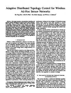
Fig. 1. Three transmission protocols. (a) Direct transmissions via a pointto-point conventional link. (b) Multi-hop transmissions via a two-hop manner occupying two time slots. (c) Cooperative transmissions via a cooperative diversity occupying two consecutive slots. The destination combines the two signals from the source and the relay to decode the information.

access control function well, e.g., the popular IEEE 802.11 MAC in most mobile devices in MANETs. Herein, interference of a link is defined as some combination of coverage of nodes involved in the transmission, which has been used in the literature [15]–[17].

In this section, we describe the network model adopted in this paper and formulate the general topology control to an optimization problem based on the network model.

Definition 1 (Node coverage). The coverage of a node refers to its neighbors, i.e., 𝐶𝑜𝑣(𝑢) = 𝒱𝑁 (𝑢) for node 𝑢. In the physical meaning, it includes nodes covered by this node.

A. Network Model

Definition 2 (Link interference). It refers to the number of influenced nodes during the transmission.

A network topology involves two aspects: network nodes and the connection links among them. In general, a MANET can be mapped into a graph 𝒢(𝒱, ℰ), where 𝒱 is the set of nodes in the network and ℰ is the edge set representing the wireless links. A link is generally composed of two nodes which are in the transmission range of each other in classical MANETs. The topology of such a classical MANET is parameterized by some controllable parameters, which determine the existence of wireless links directly. Usually, these parameters can be transmit power and antenna directions, etc. By the introduction of cooperative communications, we consider three transmission modes in MANETs: direct transmissions (Fig. 1(a)), multi-hop transmissions (Fig. 1(b)) and cooperative transmissions (Fig. 1(c)). Direct transmissions and multi-hop transmissions can be regarded as special types of cooperative transmissions. A direct transmission utilizes no relays while a multi-hop transmission does not combine signals at the destination. Obviously from Fig. 1(c), it is known that the cooperative channel is a virtual multiple input single output (MISO) channel, where spatially distributed nodes are coordinated to form a virtual antenna to emulate multi-antenna transceivers. A cooperative transmission consists of two types of channels: broadcast channel and multiple access channel. The channel time is divided into two orthogonal consecutive slots to implement cooperative transmissions [5]. The source broadcasts its messages to the relay and destination in the first slot, and the destination obtains the signals from the source and the relay via multiplexing technology in the second slot. Let them be 𝑆, 𝑅 and 𝐷 respectively. As a result, the link is presented by (𝑆, 𝑅, 𝐷) and the topology becomes 𝒢𝐶 (𝒱, ℰ𝐶 ) where ℰ𝐶 = {(𝑆, 𝑅, 𝐷)∣𝑆, 𝑅, 𝐷 ∈ 𝒱}. If the relay is changed, the performance of transmissions for the link is then changed. Therefore, relay selection criteria can also determine the wireless links. To evaluate the capacity for each transmission mode, we assume a Raleigh fading channel [4]. The protocol interference model [14], which confines concurrent transmissions in the vicinity of the transmitter and receiver, is adopted in this study. This model fits the medium

B. Topology control Formulation As topology control is to determine the existence of wireless links subject to network connectivity, the general topology control problem can be expressed as 𝒢 ∗ = arg max 𝑓 (𝒢) or 𝒢 ∗ = arg min 𝑓 (𝒢),

(1)

s.t. network connectivity. The above topology control problem consists of three elements, which can be formulated by a triple ⟨𝕄, ℙ, 𝕆⟩, where 𝕄 represents network model, ℙ represents the desired network property, which often refers to network connectivity for most topology control algorithms, and 𝕆 refers to the optimization objective [18]. The problem (1) uses the original network topology 𝒢, which contains mobile nodes and link connections, as the input. According to the objective function, a new good topology 𝒢 ∗ (𝒱, ℰ ∗ ) will be constructed as the output of the algorithm. 𝒢 ∗ should contain all mobile nodes in 𝒢, i.e., they have the same node set. The link connections ℰ ∗ should preserve network connectivity without partitioning the network. The structure of resulting topology is strongly related to the optimization objective function, which is 𝑓 (𝒢) in (1). For MANETs, it is difficult to collect the entire network information. Therefore, the above centralized topology control should be solved using a distributed algorithm, which generally requires only local knowledge, and the algorithm runs at every node independently. Consequently, each node in the network is responsible for managing the links to all its neighbors only. If all the neighbor connections are preserved, the end-to-end connectivity is then guaranteed via a hop-byhop manner. Given a neighborhood graph 𝒢𝑁 (𝒱𝑁 , ℰ𝑁 ), we can define a distributed topology control problem as ∗ ∗ 𝒢𝑁 = arg max 𝑓 (𝒢𝑁 ) or 𝒢𝑁 = arg min 𝑓 (𝒢𝑁 ),

(2)

s.t. connectivity to all the neighbors. The objective functions are critical to topology control problems. They may be energy consumption, interference and

2164

IEEE TRANSACTIONS ON WIRELESS COMMUNICATIONS, VOL. 10, NO. 7, JULY 2011

network capacity, or QoS provisioning under some constraints of delay and bandwidth [19]. They are achieved by adjusting some controllable parameters, such as transmission power, antenna direction, channel assignment and even cooperation level, which affect the link status. The area of energy-saving topology control has attracted a great deal of attention. Under the constraint of network connectivity, topology control adjusts the transmission range of each mobile node in order to save energy. It is pointed out in [18] that the problems of minimizing the total power consumption and minimizing the maximum power consumption are NP-hard or NP-complete. Researchers then try to resolve the complex problem into sub-optimized distributed problems, which are more feasible for MANETs. For example, the reference [20] constructs a spanner topology with regard to path energy. The approach of some approximate graph based algorithms [21]–[23] is to remove long links while preserve network connectivity in order to force nodes to use multiple short hops, which saves the energy and prolongs network lifetime [24]. It is generally agreed in the literature that the reduced graph should be sparse to mitigate collisions and packet retransmissions, leading to reduce power consumption and extend network lifetime. However, if too many edges are removed from the topology, data packets may traverse along an unacceptably long path [15]. A fundamental issue has been pointed out in [16] that the performance of a multi-hop wireless network will degrade sharply as the number of hops increases. Connecting to the nearest neighbor, which generates a nearest neighbor forest, is not sufficient to reduce interference in the network [17]. With this fact, interference-aware topology control schemes emerge [15]–[17]. It is assumed that reducing interference can increase network capacity, which is an important resource for multi-hop wireless networks. The capacity of such a network is revealed to be decreased as the number of nodes in the network increases [14]. To this end, [25] proposed a capacity-aware topology control. It confines the degree of each node in the network to reduce interference and thus increase network capacity. It shares the same principle as interference-aware topology control, but without connectivity guarantee. However, reducing interference merely is not sufficient for network capacity improvement. Some recent excellent works also address the impacts of physical layer cooperative communications on upper layer performance in wireless networks [26]–[29]. They investigate the joint effects of relay assignment and routing, which are different from the network topology control issues studied in this paper. Our previous work [30] shows that topology control can affect network capacity significantly. Based on the observations in [30], we propose the COCO scheme in this paper with the objective of optimizing network capacity via topology control for MANETs with cooperative communications. Another fact in MANETs is that nodes are mobile and it is difficult to have the exact knowledge of wireless channels. The relative position of the relay and the channel state information have considerable impacts on link capacity. The noisy channel estimate may result in inaccurate link capacity calculation and worst relay selection. When nodes are moving, the topology needs to be reconfigured in time to track the changes.

III. C APACITY-O PTIMIZED C OOPERATIVE T OPOLOGY C ONTROL Based on the topology control formulation in the previous section, we will detail the design of COCO to maximize network capacity in this section. The network capacity expression is used as its objective function, which takes link capacity and interference into consideration. The network connectivity and path length are regarded as constraints for the optimization problem. The COCO scheme described in this section formulates topology control as a discrete stochastic optimization problem. A discrete stochastic approximation approach is then adopted to solve the problem. This approach is easily improved to track time-varying changes. Therefore, network topology is reconfigured in time. Before addressing COCO, we introduce some definitions to be used in the discussion. Definition 3 (Network capacity). Network capacity refers to the maximum achievable throughput of bits per second for each node on average that can be sent to its destination. The network capacity defined here includes all the end-toend throughput in the network, and it is in fact the average throughput capacity per node. A. Objective Function As an optimization problem, the objective function is the most paramount component. In COCO, the objective function is set to reflect the state of network capacity. As concluded in [30], the expected network capacity is determined by various factors. On one hand, link capacity is one of the main factors. In practice, we adopt a data rate, called outage capacity, which is supported by a small outage probability 𝜀, to stand for the link capacity. The study in [4] shows that cooperative transmissions do not always outperform direct transmissions. If there exists no such a relay that makes cooperative transmissions have larger outage capacity, we rather transmit information directly or via multi-hops. For this reason, COCO determines the best link block (see Fig. 1) and the best relay to optimize link capacity. On the other hand, other nodes in the transmission range have to be silent in order not to disrupt the transmission due to the open shared wireless media. The affected nodes include the coverage of the source (see Definition 1), the coverage of the destination, as well as the coverage of the relay. Interference, which refers to the affected nodes, also has a significant impact on network capacity. Higher interference reduces simultaneous transmissions in the network, thus reduces the network capacity, and vice versa. Link capacity and interference model vary for different links (Fig. 1). They are discussed in the following. 1) Direct transmissions: A direct transmissions is the conventional point-to-point transmission. Let 𝛾0 , 𝛾1 and 𝛾2 denote the received SNRs from the source to the destination, from the source to the relay and from the relay to the destination, respectively. Given a small outage probability 𝜀, its outage link capacity [4] is given by 𝜀 = log2 (1 + 𝛾0 ln 𝐶𝐷𝑇

1 ). 1−𝜀

(3)

GUAN et al.: CAPACITY-OPTIMIZED TOPOLOGY CONTROL FOR MANETS WITH COOPERATIVE COMMUNICATIONS

Only two nodes are involved in the direct transmission. Therefore, the interference set of a direct transmission is the union of coverage sets of the source node and the destination node: (4) 𝐼𝐷𝑇 = 𝐶𝑜𝑣(𝑆) ∪ 𝐶𝑜𝑣(𝐷). According to Definition 2, the interference is set to ∣𝐼𝐷𝑇 ∣, the size of the interference set. 2) Multi-hop transmissions: The multi-hop transmission here is actually a two-hop transmission. It consumes two time slots. In the first slot, messages are transmitted from the source to the relay and the messages will be forwarded to the destination in the second slot. The mutual information of a multi-hop transmission link is calculated by 1 𝑅𝑀𝑇 = min{𝑅𝑆→𝑅 , 𝑅𝑅→𝐷 }. 2 The outage probability is 1

(5)

1

𝑜𝑢𝑡 𝑃𝑀𝑇 = 1 − 𝑢 𝛾1 + 𝛾2 ,

(6)

2𝑅

where 𝑢 = 𝑒−(2 −1) and 𝑅 is the link data rate. 𝑜𝑢𝑡 If 𝑃𝑀𝑇 = 𝜀, the outage capacity then is 𝜀 𝐶𝑀𝑇 =

1 log2 (1 + 2

1 𝛾1

1 +

1 𝛾2

ln

1 ). 1−𝜀

(7)

The multi-hop transmission mode for a link is composed of two hops. The transmission of each hop has its own interference, which happens in different slots, where the interference sets in slots are 𝐼𝑆→𝑅 = 𝐶𝑜𝑣(𝑆) ∪ 𝐶𝑜𝑣(𝑅) and 𝐼𝑅→𝐷 = 𝐶𝑜𝑣(𝑅) ∪ 𝐶𝑜𝑣(𝐷). Since the transmissions of the two hops cannot occur simultaneously but in two separate and consecutive time slots, the end-to-end interference set of the multi-hop link is determined by the maximum of the two interference sets, i.e., 𝐼𝑀𝑇 = max{𝐼𝑆→𝑅 , 𝐼𝑅→𝐷 }.

(8)

3) Cooperative transmissions: This study uses the fixed decode-and-forward (DF) relaying scheme with only one best relay, which is selected proactively before transmissions. In the DF relaying, the relay node decodes and re-encodes the signal from the source, and then forwards it to the destination. The two signals of the source and the relay are decoded by maximal rate combining (MRC) at the destination. Its maximum instantaneous end-to-end mutual information [4] is 1 min{𝑅𝑆→𝑅 , 𝑅𝑀𝑅𝐶 }. 2 The outage probability is given by 𝑅𝐶𝑇 =

(9)

2165

neighbors of the relay and the destination have to be silent so as to ensure successful receptions at both the relay and the destination. The interference set of broadcast channel in the first transmission period is 𝐼𝑏𝑟𝑐 = 𝐼𝑆→𝑅 ∪ 𝐼𝑆→𝐷 = 𝐶𝑜𝑣(𝑆)∪𝐶𝑜𝑣(𝑅)∪𝐶𝑜𝑣(𝐷). The multiple access channel also consists of two point-to-point links: 𝑆→𝐷 and 𝑅→𝐷, which are active in separate time slots. Its interference is 𝐼𝑚𝑎 = max{𝐼𝑆→𝐷 , 𝐼𝑅→𝐷 } = max{𝐶𝑜𝑣(𝑆) ∪ 𝐶𝑜𝑣(𝐷), 𝐶𝑜𝑣(𝑅) ∪ 𝐶𝑜𝑣(𝐷)}. Now, we can derive the interference set of cooperative transmissions as 𝐼𝐶𝑇 = max{𝐼𝑏𝑟𝑐 , 𝐼𝑚𝑎 } = 𝐶𝑜𝑣(𝑆) ∪ 𝐶𝑜𝑣(𝑅) ∪ 𝐶𝑜𝑣(𝐷).

(12)

Direct transmissions and multi-hop transmissions can also be considered as special types of cooperative transmissions. For direct transmissions, we assume that the relay is also the source, while the direct signal is ignored at the destination for multi-hop transmissions. Given a node identified by 0 and its neighbor set 𝒱𝑁 = {1, 2, ⋅ ⋅ ⋅, 𝑚}, the selected relay set for all its neighbors is 𝜽 = (𝜃1 , 𝜃2 , ⋅ ⋅ ⋅, 𝜃𝑚 ). Let Θ denote the set of all the possible relays for its neighbors. Therefore, 𝜽 ∈ Θ. For any one of its neighbors 𝑗, suppose that 𝜃𝑗 ∈ Θ𝑗 = {0, 1, ⋅ ⋅ ⋅, 𝑚, 𝑚 + 1, ⋅ ⋅ ⋅, 2𝑚} − {𝑗, 𝑚 + 𝑗}. The link outage capacity attains to ⎧ 1 𝜃𝑗 = 0  2 (1 + 𝛾0 ln 1−𝜀 ) ⎨log 1 1 log (1 + ln ) 0 < 𝜃𝑗 ≤ 𝑚 2 𝐶𝜀 (𝜸(𝜃𝑗 ))= 2 (13) 𝑢𝜀 (𝜸(𝜃𝑗 ))  1 ⎩ 12 log2 (1+ 1 1 1 ln 1−𝜀 ) 𝑚 < 𝜃 ≤ 2𝑚, 𝑗 + 𝛾1

𝛾2

where 𝜸(𝜃𝑗 ) = (𝛾0 , 𝛾1 , 𝛾2 ), and 𝑢𝜀 (𝜸(𝜃𝑗 )) is derived by 𝑜𝑢𝑡 𝑃𝐷𝐹 = 𝜀 in (10). Herein, (13) combines the three types of transmission protocols together. The case 𝜃𝑗 = 0 corresponds to direct transmissions. For the other two relaying cases, if 𝜃𝑗 is selected for cooperative relaying, 𝜃𝑗 + 𝑚 is the same selected relay node but for multi-hop relaying. In the smart selective decode-and-forward (SSDF) relaying [4], a relay is used only when relaying is beneficial. The case of not using the relay corresponds to the direct transmission in (13). Distinct from SSDF, in addition to considering the cooperative transmission, the objective function of COCO extends the linkwide behavior into a network-wide perspective by taking into account the interference. Based on the above discussion, the interference set of a link in MANETs with cooperative communications is equal to ⎧ ⎨ 𝐼𝐷𝑇 (𝜃𝑗 ), 𝜃𝑗 = 0 (14) 𝐼𝐶𝑇 (𝜃𝑗 ), 0 < 𝜃𝑗 ≤ 𝑚 𝐼(𝜃𝑗 ) = ⎩ 𝐼𝑀𝑇 (𝜃𝑗 ), 𝑚 < 𝜃𝑗 ≤ 2𝑚.

(11)

Link data rate and interference are the primary factors which determine network capacity. Since the links in cooperative networks are determined by relay selection, on the basis of Definition 3 and the discussions in [30] the objective function is set as follows to optimize network capacity, ∑ 𝐶𝜀 (𝜸(𝜃𝑗 )) . (15) 𝑓 (𝜸(𝜽)) = ∣𝐼(𝜃𝑗 )∣

The interference of a cooperative transmission is a bit complicated. In the broadcast period, not only the covered neighbors of the source have to be silent, but also the covered

Assume that the MAC function can avoid interference among different adjacent links. Therefore, each node can independently determine its relay. In this sense, we get

𝑜𝑢𝑡 𝑃𝐶𝑇

=1+

𝛾0 𝛾10 + 𝛾11 𝛾2 𝑢

1−

1

1

− 𝑢 𝛾1 + 𝛾2 𝛾0 𝛾2

.

(10)

𝑜𝑢𝑡 Let 𝑃𝐷𝐹 = 𝜀 in (10), we get a 𝑢𝜀 . Then, the outage capacity is expressed as 𝜀 = 𝐶𝐶𝑇

1 1 log2 (1 + ln ). 2 𝑢𝜀

𝑗∈𝒱𝑁

2166

IEEE TRANSACTIONS ON WIRELESS COMMUNICATIONS, VOL. 10, NO. 7, JULY 2011

∑ 𝐶𝜀 (𝜸(𝜃𝑗 )) ∑ 𝐶 (𝜸(𝜃 )) max = max 𝜀∣𝐼(𝜃𝑗 )∣𝑗 . The topology control ∣𝐼(𝜃𝑗 )∣ formulation then is equivalent to 𝜃𝑗∗ = arg max 𝑔(𝜸(𝜃𝑗 )), for all 𝑗 ∈ 𝒱𝑁 , 𝜃𝑗 ∈Θ𝑗

where 𝑔(𝜸(𝜃𝑗 )) =

𝐶𝜀 (𝜸(𝜃𝑗 )) . ∣𝐼(𝜃𝑗 )∣

(16)

(17)

As we can see from the objective function (17), COCO determines the best type of transmission links and the best relay to optimize network capacity. The maximizer in (16) is actually such a scheme for the link 𝑖→𝑗 that results in high link capacity and low interference to the network. The topology control problem (15) is divided into 𝑚 independent and parallel subproblems (16). Distributed and parallel computing can be adopted to accelerate the computational speed. For the specific 𝑗th optimization subproblem, the solution space size Θ𝑗 is 𝑚⋅(2𝑚−1), much smaller than (2𝑚−1)𝑚 of Θ in (15). As a result, the computational load is dramatically reduced. B. Constraints At least two constraint conditions are necessarily taken into consideration in the capacity-optimized topology control problem. One is network connectivity, which is also the basic element ℙ in the topology control triple ⟨𝕄, ℙ, 𝕆⟩. Actually, the end-to-end network connectivity is guaranteed via a hop-by-hop manner in the objective function. Every node is in charge of the connections to all its neighbors. If all the neighbor connections are guaranteed, the end-to-end connectivity in the whole network can be preserved [20]. The other aspect that determines network capacity is the path length. An end-to-end transmission that traverses more hops will import more data packets into the network. Although path length is mainly determined by routing, COCO limits dividing a long link into too many hops locally. The limitation is two hops due to the fact that only two-hop relaying is adopted. In practice, the exact knowledge of the channel status may not be available. Instead, we typically have a noisy estimate of the channel SNR. Thus, the topology control problem becomes a discrete stochastic optimization problem. In the next subsection, we will solve this problem via a discrete stochastic approximation approach. C. Discrete Stochastic Approximation Approach for COCO An intuitive brute force approach to solve the discrete stochastic problem in (16) is as follows. For each possible relay candidate 𝜃𝑗 ∈ Θ𝑗 , we compute 𝑁 estimates of its objective function 𝑔(𝜸(𝜃𝑗 )). The empirical average is then used to approximate the exact value of 𝑔(𝜸(𝜃𝑗 )), i.e., 𝑔ˆ𝑁 (𝜃𝑗 ) =

𝑁 1 ∑ 𝑔(𝑛, 𝜃𝑗 ). 𝑁 𝑛=1

(18)

By the strong law of large numbers, 𝑔ˆ(𝑛, 𝜃𝑗 ) is almost surely approximate to 𝐸[𝑔(𝑛, 𝜃𝑗 )] as 𝑁 grows to infinity. Based on the estimates, the global maximizer of the objective function is exhaustively searched by 𝜃𝑗∗ = arg max 𝑔ˆ𝑁 (𝜃𝑗 ). Apparently, 𝑁 estimates for each relay candidate would lead to totally

𝑁 × ∣Θ𝑗 ∣ estimates. In fact, the computations of non-optimal estimates are wasted since we are only interested in the estimates of the optimal relay candidate. In this sense, the brute force approach is inefficient, especially when in a dense network and the nodes are moving. A discrete stochastic approximation approach [10]–[13] can be used to solve (16). Let 𝜃𝑗 [𝑛] denote the selected relay at 𝑛th iteration and 𝒆𝜃𝑗 [𝑛] be a unit 𝒱𝑁 × 1 vector with a one in the 𝜃𝑗 [𝑛]-th position and zeros elsewhere. A probability vector 𝝅[𝑛] = [𝜋[𝑛, 1], ⋅ ⋅ ⋅, 𝜋[𝑛, ∣𝒱𝑁 ∣]], which is updated at each iteration, is used to represent the state occupation probabilities for all the relay candidates. 𝜃𝑗 [𝑛] is the selected relay for neighbor 𝑗 at the 𝑛th iteration. Algorithm 1. Basic COCO algorithm Step 0 (Initialization) At iteration 𝑛 = 0, select an initial state of the algorithm 𝜃𝑗 [0] ∈ Θ𝑗 randomly and set 𝝅[0] = 𝒆𝜃𝑗 [0] . Initialize estimate of optimal relay selection as 𝜃ˆ𝑗 [0] = 𝜃𝑗 [0]. Step 1 (Sampling and evaluation) Evaluate 𝑔(𝜃𝑗 [𝑛]) given 𝜃𝑗 [𝑛] at iteration 𝑛. Generate an alternative 𝜃˜𝑗 [𝑛] ∈ 𝒩𝜃𝑗 [𝑛] uniformly and evaluate 𝑔(𝜃˜𝑗 [𝑛]). Step 2 (Acceptance) IF 𝑔(𝜃˜𝑗 [𝑛]) > 𝑔(𝜃𝑗 [𝑛]) 𝜃𝑗 [𝑛 + 1] = 𝜃˜𝑗 [𝑛] ELSE 𝜃𝑗 [𝑛 + 1] = 𝜃𝑗 [𝑛] END IF Step 3 (Update empirical state occupation probability) 𝝅[𝑛 + 1] = 𝝅[𝑛] + 𝜇[𝑛 + 1](𝒆𝜃𝑗 [𝑛+1] − 𝝅[𝑛])

(19)

1 𝑛.

with a decreasing step 𝜇[𝑛] = Step 4 (Update estimate of optimal maximizer) (𝑛+1) (𝑛) ] > 𝜋[𝑛 + 1, 𝜃ˆ𝑗 ] IF 𝜋[𝑛 + 1, 𝜃𝑗 𝜃ˆ𝑗 [𝑛 + 1] = 𝜃𝑗 [𝑛 + 1] ELSE 𝜃ˆ𝑗 [𝑛 + 1] = 𝜃ˆ𝑗 [𝑛] END IF Go back to Step 1. Each iteration of the above algorithm consists of several steps. In Step 1, the algorithm randomly picks up one relay from 𝒩𝜃𝑗 [𝑛] = Θ𝑗 − {𝜃𝑗 [𝑛]} and evaluates its objective value. For rigorously proving the convergence and efficiency of the algorithm, we adopt independent samples to estimate the objective function. That is, the channel is estimated independently at every iteration. The randomly selected relay will be accepted as the current visiting state in the next step if its objective value is larger than the objective value of the previous state. In Step 3, the empirical occupation probabilities of all the states in 𝝅[𝑛] are updated. The element 𝜋[𝑛, 𝜃𝑗 [𝑛]] of 𝝅[𝑛] equals to 𝜋[𝑛, 𝜃𝑗 [𝑛]] =

# of state visits of 𝜃𝑗 [𝑛] so far . 𝑛

(20)

𝜃ˆ𝑗 [𝑛] is set to the most frequently visited state according to the state probability vector 𝝅[𝑛]. The visited state sequence {𝜃𝑗 [𝑛]} is a Markov chain on the state space Θ𝑗 since it is determined by the last state and

GUAN et al.: CAPACITY-OPTIMIZED TOPOLOGY CONTROL FOR MANETS WITH COOPERATIVE COMMUNICATIONS Multihop transmissions

Direct transmissions 0.35

Empirical distribution function Fn

0.25 Probability

Cooperative transmissions 0.35

Fit distribution function F

0.3

0.2 0.15 0.1 0.05 0

0.35

0

Fig. 2.

0.3

0.3

0.25

0.25

0.2

0.2

0.15

0.15

0.1

0.1

0.05

0.05

0 0.02 0.04 0.06 0.08 0. 1 0.05 0.1 0.15 Estimated objective function g(n,s)

0 0.05

0.1

0.15

Statistical distributions of the estimated objective function.

the current sampling value. However, it is not guaranteed to converge. In the following subsection, we will prove that under some conditions, the sequence 𝜃ˆ𝑗 [𝑛] almost surely converges to the global maximizer 𝜃𝑗∗ .

2167

Theorem 1 (Global convergence). Algorithm 1 converges to the global maximizer after sufficient iterations. Proof: Suppose the mean and variance of the objective function for 𝑔(𝑛, 𝑠) are 𝐸[𝑔(𝑛, 𝑠)] = 𝜇𝑠 and 𝑉𝑎𝑟{𝑔(𝑛, 𝑠)} = 𝜎𝑠2 , respectively. We obtain a simulation statistical distribution of 𝑔(𝑛, 𝑠) in Fig. ∑ 2. Consider the empirical distribution 𝑁 function 𝐹𝑛 (𝑥) = 𝑁1 𝑖=1 1{𝑋𝑖 𝜇𝑡 if 𝑔(𝑠) > 𝑔(𝑡). Condition (21) can be rewritten as Pr{𝑔(𝑛, 𝑠) − 𝑔(𝑛, 𝑡) > 0} > Pr{𝑔(𝑛, 𝑡) − 𝑔(𝑛, 𝑠) > 0}. (25) It is equivalent to

D. Convergence Discussion The efficiency of Algorithm 1 lies in the attractive property of the algorithm. It spends more time on the global maximizer. As time goes by, it is attracted to the optimum. According to [31], the sufficient convergence condition for Algorithm 1 is as follows. Lemma 1 (Sufficient convergence conditions). Algorithm 1 converges to the global maximizer of the objective function 𝑔(𝜸(𝜃𝑗 )) if the following conditions are satisfied, Pr{𝑔(𝑛, 𝜃𝑗∗ )

> 𝑔(𝑛, 𝜃𝑗 )} > Pr{𝑔(𝑛, 𝜃𝑗 ) >

𝑔(𝑛, 𝜃𝑗∗ )}

(21)

and Pr{𝑔(𝑛, 𝜃𝑗∗ ) > 𝑔(𝑛, 𝜃˜𝑗 )} > Pr{𝑔(𝑛, 𝜃𝑗 ) > 𝑔(𝑛, 𝜃˜𝑗 )}. (22) It is pointed out in [31] that the above conditions make {𝜃𝑗 [𝑛]} a homogeneous irreducible and aperiodic Markov chain. The Markov chain spends more time on 𝜃𝑗∗ than any other states. Therefore, {𝜃ˆ𝑗 } converges almost surely to 𝜃𝑗∗ . The transition probability matrix 𝑷 = {𝑝𝑠,𝑡 } for the Markov chain {𝜃𝑗 [𝑛]} is given by 𝑝𝑠,𝑡 = Pr{𝜃𝑗 [𝑛 + 1] = 𝑡∣𝜃𝑗 [𝑛] = 𝑠} 1 = Pr{𝑔(𝑛, 𝑡) > 𝑔(𝑛, 𝑠)} ∣Θ𝑗 ∣ − 1 and 𝑝𝑠,𝑠 = 1 −

∑

(23)

𝑝𝑠,𝑡

∑ 1 Pr{𝑔(𝑛, 𝑡) > 𝑔(𝑛, 𝑠)}, ∣Θ𝑗 ∣ − 1

2 2 + 𝜎𝑔(𝑠) ) > 0}. (26) Pr{𝑁 (𝜇𝑔(𝑡) − 𝜇𝑔(𝑠) , 𝜎𝑔(𝑡)

We know that 𝜇𝑔(𝑠) = max{𝜇𝑔(𝑠) , 𝜇𝑔(𝑡) , 𝜇𝑔(𝑘) }. Then (𝜇𝑔(𝑠 )− 𝜇𝑔(𝑡) ) > (𝜇𝑔(𝑡) − 𝜇𝑔(𝑠) ). Therefore, condition (21) is satisfied due to the same variance. In the same way, condition (22) is equivalent to 2 2 Pr{𝑁 (𝜇𝑔(𝑠) − 𝜇𝑔(𝑘) , 𝜎𝑔(𝑠) + 𝜎𝑔(𝑘) ) > 0} > 2 2 + 𝜎𝑔(𝑘) ) > 0}. (27) Pr{𝑁 (𝜇𝑔(𝑡) − 𝜇𝑔(𝑘) , 𝜎𝑔(𝑡)

The following inequality is observed to hold by obtaining the mean values and variances via extensive simulations, 𝜇𝑔(𝑡) − 𝜇𝑔(𝑘) 𝜇𝑔(𝑠) − 𝜇𝑔(𝑘) √ > √ . (28) 2 2 2 2 𝜎𝑔(𝑠) + 𝜎𝑔(𝑘) 𝜎𝑔(𝑡) + 𝜎𝑔(𝑘) Therefore, condition (22) is also satisfied. In the next section, we will show that the discrete stochastic approximation approach can be improved to track the changing optimal network capacity due to mobility. IV. A DAPTIVE R ECONFIGURATION FOR T IME - VARYING T OPOLOGY

𝑡∈𝒩𝑠

=

2 2 + 𝜎𝑔(𝑡) ) > 0} > Pr{𝑁 (𝜇𝑔(𝑠) − 𝜇𝑔(𝑡) , 𝜎𝑔(𝑠)

(24)

𝑡∈𝒩𝑠

for all 𝑠, 𝑡 ∈ Θ𝑗 and 𝑠 ∕= 𝑡. Let 𝑡 = 𝜃𝑗 ∈ Θ𝑗 − {𝜃𝑗∗ } and 𝑠 = 𝜃𝑗∗ in (21). We obtain 𝑝𝑡,𝑠 > 𝑝𝑠,𝑡 , i.e., the algorithm has more chances to move into the global optimum 𝜃𝑗∗ from any other states than that in the opposite direction. Again, let 𝜃ˆ𝑗 = 𝑡, 𝜃˜𝑗 = 𝑘 (𝑘, 𝑡 ∈ Θ𝑗 −{𝜃𝑗∗ }) and 𝜃𝑗∗ = 𝑠 in (22). We obtain 𝑝𝑡,𝑠 > 𝑝𝑡,𝑘 , i.e., if the current state is not the global maximizer, it is more probable to go to the optimal state than the non-optimal state.

COCO in Algorithm 1 is developed for the topology control in static wireless networks. However, in a MANET with cooperative communications, mobile nodes are moving and the wireless environment is changing all the time. In this case, that means the optimum topology is changing from time to time. Accordingly, the topology control algorithm is required to reconfigure the network frequently in order to track the dynamic changes. The advantage of the recursive discrete stochastic approximation approach in Algorithm 1 can be applied to track the dynamic topology adaptively. The step size 𝜇 in (19) influences the tracking performance of the algorithm. It is required that 0 < 𝜇 ≤ 1 to make 𝝅[𝑛] a probability vector. If 𝜇 = 1, it means that all the previous states are forgotten. This corresponds to the brute force exhaustive off-line search, which can be regarded as an extreme case of the recursive algorithm. If 𝜇 = 0, it means the algorithm will stay in one state. In general, 𝜇 ∕= 0 unless

IEEE TRANSACTIONS ON WIRELESS COMMUNICATIONS, VOL. 10, NO. 7, JULY 2011

the algorithm reaches the optimal maximizer. For the dynamic tracking case, the step size 𝜇 should be set to a large value in order to permit moving away from the current promising state since the optimal points are changing over time. In Algorithm 1, it uses a decreasing step size 𝜇[𝑛] = 𝑛1 . It makes the algorithm become increasingly conservative to stay in the current promising state. However, with the conservative step size, the algorithm keeps the stable state even when nodes move to another positions, which changes the optimal network topology. We adopt a continuous least-mean-square (LMS)like algorithm to make the step size adaptive to the changing environment. ∂ 𝝅 𝜇 [𝑛]. The error is defined as Let 𝑱 𝜇 [𝑛] = ∂𝜇 (29)

Actually, 𝒆[𝑛+1] can be viewed as the state probability vector with a step size 𝜇 = 1. The error is the difference between current state probability and the probability with 𝜇 = 1. Then the square of the error is differentiated with respect to 𝜇, ∂ 𝜇 (𝒆 [𝑛]𝒆𝜇 [𝑛]𝑇 ) = −2(𝒆[𝑛 + 1] − 𝝅 𝜇 [𝑛])𝑇 𝑱 𝜇 [𝑛]. ∂𝜇

(30)

Differentiating equation (19), we get

(b) Grid topology

(c) Random topology

Fig. 3. Simulation scenarios. (a)10 nodes are positioned in a straight line and the interval between them is 100 meters. (b) 36 nodes in total are placed in a 6 × 6 grid, and the adjacent interval is 120 meters. (c) 30 nodes are randomly deployed in a 800 × 800 𝑚2 area. 2.5

Network capacity per node (bit/s/Hz)

𝝐𝜇 [𝑛] = 𝒆[𝑛 + 1] − 𝝅 𝜇 [𝑛].

(a) Line topology

2.5

Maximum network capacity COCO LLISE

2

Network capacity per node (bit/s/Hz)

2168

Median network capacity Worst network capacity

1.5

1.5

1

0.5

𝑱 𝜇 [𝑛 + 1] = 𝑱 𝜇 [𝑛] − 𝜇𝑱 𝜇 [𝑛] + (𝒆[𝑛 + 1] − 𝝅 𝜇 [𝑛]). (31) The rationale beyond the algorithm is to minimize the expectation of (29). Algorithm 2. COCO with adaptive step size (COCO-ASS) Substitute Step 3 of Algorithm 1 by Step 3´ (Update empirical state occupation probability) 𝝐[𝑛] = 𝒆[𝑛 + 1] − 𝝅[𝑛] 𝝅[𝑛 + 1] = 𝝅[𝑛] + 𝜇[𝑛]𝝐[𝑛] +

𝜇[𝑛 + 1] = {𝜇[𝑛] + 𝜈𝝐[𝑛]𝑇 𝑱 𝜇 [𝑛]}𝑢𝑢− 𝑱 [𝑛 + 1] = (1 − 𝜇[𝑛])𝑱 [𝑛] + 𝝐[𝑛], 𝑱[0] = 0 The above algorithm is an improved COCO algorithm by adaptive step size. 𝜈 stands for the learning rate to adjust the step size. It includes two cross-coupled adaptive algorithms: a discrete algorithm to select a capacity-optimized relay and a continuous algorithm to adjust the step size. 𝜇 is projected to an interval [𝜇− , 𝜇+ ], where 0 < 𝜇−