Cartesian GP in Optimization of Combinational Circuits with ... - VUT FIT
Recommend Documents
to optimize complex circuits, Cartesian Genetic Programming. (CGP) is employed where ... While the achievable quality of resulting design/optimization is usually very high, ... Moreover, this is a classic subtask in the logic optimization research ..
Miller and Thompson [18], [19], [20] is a widely-used method for extrinsic ..... [18] J. Miller and P. Thomson, âCartesian Genetic Programming,â in. Proc. of the 3rd ...
Combinational logic circuits (circuits without a memory): Combinational switching
networks whose outputs depend only on the current inputs. Sequential logic ...
proposed for sequential processing of LUT cascades by means of multi-way ..... The map of a sample function (a), a switch statement (b), and a dispatch table.
Automatic Discovery of RTL Benchmark Circuits with Predefined Testability .... Example of source code. The program generates a benchmark circuit according.
Cartesian genetic programming (CGP) is a branch of genetic programming which has ... A brief comparison of CGP and tree-based. GP is also performed on ...
Jerry Chih-Yuan Yang. Giovanni De Micheli. Technical Report: CSL-TR-93-584. September 1993. This research is sponsored by NSF and DEC under a PYI ...
the physical design of the REPOMO32 chip is robust enough to keep the functionality of all .... Implementation of novel concepts for testing and diag- nosing of ...
AbstractâIn this paper we research the possibility of automated combinational logic circuit (CLC) design using evolutionary computation. We propose and ...
circuits are conventionally constructed by adding checking logic around an un- modified original output of the circuit. Garvie utilized the evolutionary algorithm.
Evolutionary Design of Synthetic RTL Benchmark Circuits. ZdenÄk Kotásek, Tomáš ... The program generates a benchmark circuit according to the predefined ...
2.2 ENERGY AND ZERO-CROSSING RATE. Another widely used method is a method based on the comparison of the energy and zero-crossing rate (ZCR) of ...
1. Evolutionary Approach to Approximate Digital. Circuits Design. Zdenek Vasicek and Lukas Sekanina. AbstractâIn approximate computing, the requirement of ...
full-adder. In circuit development two half-adders can be employed to form a .... A
combinational circuit of full-subtractor performs the operation of subtraction of.
Half adder is a combinational logic circuit with two input and two output. The half
... The disadvantage of a half subtractor is overcome by full subtractor. The full ...
Logic Circuit Lab. Lab #5; Page 1/3. Spring 2003. Combinational Circuits Using
VHDL ... The text book Digital Design: Principles and Practices, 3rd Edition by ...
Common Combinational Logic Circuits. • Adders. – Subtraction typically via 2s
complement addition. • Multiplexers. – N control signals select 1 of up to 2N
inputs ...
Examples for combinational digital circuits are Half adder,. Full adder, Half
subtractor, Full subtractor, Code converter, Decoder, Multiplexer,. Demultiplexer ...
Modeling Combinational Logic. Circuits. Debdeep Mukhopadhyay. IIT Madras ...
Circuit Structure. Second circuit has a shorter critical delay (longest path delay)!
CSZ Computer Systems note 9. Combinational Logic Circuits. Computer systems
are built from binary digital logic circuits: circuits in which each signal has only ...
Mostafa Abd-El-Barr, Sadiq M. Sait, Bambang A. B. Sarif, and Uthman Al-Saiari. Computer Engineering Department. KFUPM, Dhahran-31261, Saudi Arabia.
[17] Vassilev, V., Job, D., and Miller, J. F., âTowards the Automatic Design of ... [32] Miller, J. F. and Thomson, P., âCartesian Genetic Programming,â in [Proc. of ...
Driven by ever increasing requirements from the video game industry, GPUs have ... But in order to utilize such power, programmer must consider a variety of differences: .... in mastering CUDA and involving GPU in simple tasks that can be efficiently
Cartesian GP in Optimization of Combinational Circuits with ... - VUT FIT
Thousands of Gates. Zdenek Vasicek. Brno University of Technology, Faculty of Information Technology,. IT4Innovations Centre of Excellence, Brno, Czech ...
Cartesian GP in Optimization of Combinational Circuits with Hundreds of Inputs and Thousands of Gates Zdenek Vasicek Brno University of Technology, Faculty of Information Technology, IT4Innovations Centre of Excellence, Brno, Czech Republic Email: [email protected] Abstract. A new approach to the evolutionary optimization of large digital circuits is introduced in this paper. In contrast with evolutionary circuit design, the goal of the evolutionary circuit optimization is to minimize the number of gates (or other non-functional parameters) of already functional circuit. The method combines a circuit simulation with a formal verification in order to detect the functional inequivalence of the parent and its offspring. An extensive set of 100 benchmarks circuits is used to evaluate the performance of the method as well as the utilized evolutionary approach. Moreover, the role of neutral mutations in the context of evolutionary optimization is investigated. In average, the method enabled a 34% reduction in gate count even if the optimizer was executed only for 15 minutes.
1
Introduction
One of the most serious problems of evolvable hardware, especially in the area of evolutionary synthesis of logic circuits, is a very time consuming evaluation of candidate circuits. This problem is known as the problem of scalability. It causes that the evolutionary synthesis can handle only small and usually simple problems that are far from real-world problem instances. In order to improve the scalability of evaluation, application-specific hardware as well as software methods were designed to increase the performance of the evolutionary optimization and design of logic circuits, see e.g. [2, 4–6, 9]. These methods enabled to increase the complexity of problem instances that can be solved in a reasonable time. Unfortunately, the methods are not scalable. The time needed to evaluate a candidate solution usually grows exponentially with the increasing number of primary inputs, but the accelerators are usually able to deliver a linear speedup only. Introducing more domain knowledge and utilizing more advanced evolutionary methods seem to be the only viable approach for dealing with the real-world problem instances. A breakthrough in the field of evolvable hardware was achieved with the introduction of a method which ties formal verification together with evolutionary optimization and substantially reduces the scalability issue of the evaluation [7]. Vasicek and Sekanina demonstrated that the previous empirical limitation of evolutionary design represented by a digital circuit having about 20 inputs can easily be overcome.
The goal of this paper is to introduce and evaluate a new approach which extends the method published in [8]. The advantage of the improved approach, which combines formal verification with simulation-based verification, is the ability to optimize digital circuits (i.e. to reduce the number of gates, improve power consumption, delay, etc.) represented at the gate level having hundreds of inputs and consisting of thousands of gates. The circuits of such a complexity have never been either evolved or optimized in the field of evolvable hardware at the gate level directly. In contrast with previously published works which are evaluated using a few benchmark circuits, an extensive set of 100 benchmarks circuits is used to evaluate the performance the proposed method. In addition to that, we would like to identify the key weaknesses of the evolutionary approach and propose future directions that could help the evolutionary approaches to penetrate into the area of real applications. In particular, we analyzed the role of neutral mutations in the context of evolutionary optimization.
2 2.1
Evolutionary optimization of combinational circuits Cartesian Genetic Programming
Cartesian Genetic Programming can be considered as one of the most efficient methods for evolutionary design and optimization of digital combinational circuits [3]. A candidate circuit is represented using an array of gates arranged in a matrix consisting of nc columns and nr rows. Each gate can be connected either to the output of a gate placed in previous l columns or to one of the circuit inputs. It means that no feedback is allowed. This requirement guarantees that only the combinational circuits will arise. Each gate is programmed to perform one of na -input functions defined in the set Γ . The number of circuit inputs, ni , and outputs, no , is fixed. Every candidate circuit is encoded using nc · nr · (na + 1) + no integers. The main advantage of the utilized encoding is that the size of phenotype is variable even if the size of chromosome is fixed. The variability is given by the fact that some nodes need not be employed in encoded circuit. CGP operates with the population of 1+λ individuals. The initial population is usually seeded randomly. However, in order to optimize a known circuit (i.e. to minimize the number of gates), it is useful to seed the initial population by this circuit. Every new population consists of the best individual of the previous population and its λ offspring individuals. The offspring individuals are created using a point mutation operator which modifies h randomly selected genes of the chromosome. An important rule for selection of the new parent is utilized. In the case when two or more individuals can serve as the parent, an individual which has not served as the parent in the previous generation will be selected as a new parent. This strategy is important because it ensures the diversity of population [3]. The algorithm is terminated when the maximum number of generations is exhausted or a sufficient solution is obtained. In case of digital circuit evolution, the fitness value of a candidate circuit is defined as follows. If a fully functional solution is evolved, the fitness value
consist of the number of correct output bits obtained as response for all possible assignments to the inputs plus the number of unused CGP nodes. Otherwise, only the number of correct output bits is used. It means that the evolution has to discover a perfectly working solution firstly while the size of circuit is not important. Then, the number of gates is optimized. Similarly, delay or power consumption may be optimized. 2.2
Speeding up the fitness evaluation using a SAT solver
Contrary to the evolutionary design, the evolutionary optimization of digital circuits begins with the population seeded by a fully functional circuit. Usually, the goal is to minimize the number of gates. The most important feature of the evolutionary optimization is that each candidate solution created by means of genetic operators must be functionally equivalent with its parent in order to be further evaluated. This feature was utilized in [7] and furthermore elaborated in [8]. Equivalence checking was applied to decide whether a candidate circuit is functionally correct or not. In order to calculate the fitness value, the candidate circuit as well as its parent are converted to a Boolean formula whose satisfiability is investigated using a SAT solver. In fact, the parent serves as a golden reference for combinational equivalence checking. The advanced version, introduced in [8], utilizes another feature of evolutionary-based approach – the knowledge of the points in a candidate circuit that may break the correct function. This information is available because each offspring was created by a mutation from its parent. Hence, only a ‘difference‘ (so-called cone of influence) between the candidate solution and its parent can be calculated. The Boolean formula can be derived from this ‘difference‘. Since the cone of influence usually represents only a small part of the candidate circuit, the time needed to decide the satisfiability of the Boolean formula can significantly be reduced. If the obtained Boolean formula is satisfiable, a negative fitness value is assigned to the candidate circuit because the candidate circuit captures a different Boolean function. Otherwise, the candidate circuit is functionally equivalent with the specification and the fitness value is calculated according to the objective of the optimization. For example, the number of utilized gates was used in [7, 8]. The usage of SAT solver helped to reduce the most time consuming part of the evolutionary algorithm, the evaluation of candidate solutions. In contrast with a common fitness function based on computing a Truth table, the time of evolution was reduced by several orders depending on the circuit parameters [8].
3
Proposed method
In order to improve the performance of the evolutionary optimizer, i.e. to increase the number of candidate solutions that can be evaluated within a period of time, we suggest to combine SAT solver with a circuit simulator which will be used to disprove the equivalence between a candidate solution and its parent. This approach is based on the assumption that the time needed to simulate a given
candidate circuit using NV (NV 2ni ) test vectors (tsim ) is significantly lower than the time which is consumed by a SAT solver (tsat ). The correctness of a candidate solution is determined as follows. Firstly, a circuit simulator is applied to the difference circuit between a candidate solution and its parent (difference circuit is calculated according to [8]). The simulator can use up to NV randomly generated test vectors. If there is a test vector which evaluates the output of the difference to one, the simulator is terminated and a negative fitness value is assigned to the corresponding candidate solution. Since it is guaranteed that the candidate solution is not functionally equivalent with its parent, it is not necessary to call SAT solver to prove that fact. Otherwise, when all NV test vectors are applied and the output of the difference evaluates to zero in all the cases, a SAT solver has to be used to prove or disprove the equivalence because the limited number of test vectors cannot guarantee that there is not a vector that differentiates the circuits. The speedup of the proposed method combining a simulator and SAT solver can be defined as follows: gain =
1 tsat = , tsim + σf ail tsat tsim /tsat + σf ail
(1)
where σf ail = [0, 1] is a coefficient which determines the fail-rate of the simulationbased equivalence checking. The σf ail may also be understood as the probability of occurence of an undetected fault. If we want to maximize the gain, i.e. the overall performance of the optimizer, we need to minimize not only the value of the ratio tsim /tsat , but also the value of σf ail . Even if the simulator is e.g. 1000 times faster than SAT solver, a neglible improvement will be achieved if the value of σf ail is close to one. The value of tsim as well as σf ail depend on the number of test vectors that can be used in the simulator to disprove the equivalence. While tsim increases linearly with increasing NV and the size of the difference entering the simulator, σf ail decreases with increasing NV . Hence, appropriate value of NV has to be determined in order to maximize the gain.
4
Experimental results
4.1
Benchmark circuits
In order to evaluate the performance of the proposed method, we utilized a set of 100 randomly chosen circuits form QUIP, WLSI and ACM/SIGDA benchmark set (only circuits with 15 and more primary inputs are considered). These circuits were synthesized and optimized by ABC 1 using ‘choice’ script. The result of ABC was utilized as the input to the evolutionary optimizer. The basic parameters of the benchmark circuits are given in Figure 1. The circuits are arranged according to the increasing complexity. The complexity is expressed as a time needed to evaluate a candidate solution using a common 1
ABC is a system for sequential synthesis and verification by A. Mishchenko.
NPI NPO
103
106
NG
105 104
102
103 102 1
5
10
15
20
25
30
35
40
45
50
55
60
65
70
75
80
85
90
95
NG
NPI, NPO
101
100
Fig. 1. The number of primary inputs (NP I ), primary outputs (NP O ) and gates (NG , right axis) for each benchmark circuit. The X-axis contains the index of benchmark circuit. The benchmarks are arranged according to the increasing complexity expressed as 2NP I NG . Note that both Y-axes have a logarithmic scale. 3
fitness function (i.e. the fitness function based on a truth table). In such a case, the evaluation time is dependent on two factors: the number of primary inputs (NP I ), and the number of gates (NG ). As the time needed to evaluate a candidate solution increases exponentially with the increasing number of primary inputs, NP I represents the key parameter which has a great impact on the total time. The least complex circuit, ‘alcom‘ circuit with index 1, consists of 106 gates and utilizes 15 primary inputs and 38 outputs. The most complex circuit, audio codec controller ‘ac97 ctrl‘ with index 100, contains 16158 gates and uses 2176 inputs and 2136 outputs. One half of the benchmark circuits have more than 50 primary inputs and consist of more than 1000 gates. 4.2
Role of neutral mutations
The objective of the first experiment was to confirm or reject hypothesis about the importance of neutral mutations in evolutionary optimization of combinational circuits. Two variants of the mutation operator were implemented in order to evaluate the significance of neutrality. The first implementation does not impose any special limitations on the mutation operator. The only requirement is to modify the value of a randomly chosen gene to a different one (but legal). On the other hand, three restrictions are applied in the second implementation: (1) inactive gates are never modified; (2) it is not possible to connect an active gate (or primary output) to an inactive gate; (3) the gene which encodes the connection of the second input of a single-input gate is never mutated. These restrictions were introduced in order to mitigate the neutral mutations. The CGP parameters were chosen as follows: nc = NG , nr = 1, l = NG , λ = 1, h = 2, Γ = {BUF, INV, AND, OR, XOR, NAND, NOR, XNOR}. These parameters were chosen according to the [8]. No redundancy in CGP encoding is used; the number of nodes is equal to the size of a benchmark circuit obtained 3
The list of benchmark circuits is available at http://www.fit.vutbr.cz/∼vasicek/gp15
from ABC. The goal of CGP is to minimize the number of utilized gates, i.e. the fitness value is equal to the number of active CGP nodes. The fitness function utilizes SAT solver only. In order to perform a statistical evaluation, fifteen independent evolutionary runs were executed for each benchmark circuit. Note that median value will be used to analyze the impact of a particular parameter because no Gaussian distribution can be observed among the benchmarks. The evolution is terminated after 15 minutes4 . We do not use the number of evaluations as a termination condition because this number is very sensitive to the structural properties of an optimized circuit and it is impossible to determine an appropriate value in advance. The performance of both approaches is evaluated using the number of generations (Gimpr ) that enabled an improvement of the fitness value. This parameter can be seen as a measure of mutation operator’s performance (i.e. the ability to generate a candidate solution which is valid and simultaneously improved). The reason behind the usage of this metric is that the number of evaluations cannot be compared directly because the neutral mutations are detected and the created candidate solutions do not enter the time-consuming fitness evaluation procedure (it is guaranteed that they have the same fitness value as their parent) resulting in the fact that significantly more generations can be produced if the occurrence of neutral mutations is high. Let G = Gvalid + Ginvalid be the total number of generations where Gvalid is the number of generations in which a valid candidate solution (i.e. functionally equivalent with a parental circuit) is generated from a parental solution by applying the mutation operator. Then, Gvalid can be expressed as Gvalid = Gimpr + Gnoimpr + Gneutral , where Gneutral is the number of neutral mutations in the sense defined in previous paragraphs. Gnoimpr represents the candidate solutions in which at least a single gene was changed but the fitness value remained unchanged. Note that Gneutral = 0 in the second implementation because no neutral mutations are allowed. The evaluation of both variants of the mutation operator is shown in Figure 2. The performance is expressed as the ratio Gimpr /(Gvalid −Gneutral ) calculated at the end of each 15-minute evolutionary run, averaged over all fifteen runs. Despite the stochastic nature of evolutionary algorithm which leads to some variances (see the error bars in Figure 2 showing the magnitude of standard deviation), we can conclude that the performance of both implementations is almost identical. In average, 2.34% of valid generations were produced when the neutral mutations were enabled and 2.42% for the opposite case. For 75 benchmarks, the variant with disabled neutral mutations performs approx. (30 ± 35) % better in average. The performance was worsened in 25 cases by approx. (9 ± 10) % in average. According to the obtained results, we can conclude that it has no advantage to support neutral mutations in this scenario (i.e. if the goal is to minimize the number of gates in a fully functional circuit). In fact, the neutral mutations have a negative impact on overall performance because the probability of mutation of 4
A PC equipped with Intel Xeon X5670 (24 cores, 2.93 GHz, 12 MB cache), 32 GB RAM and 64-bit CentOS Linux was used.
14%
neutral mutations enabled disabled
12% 10% 8% 6% 4% 2% 0%
1
5
10
15
20
25
30
35
40
45
50
55
60
65
70
75
80
85
90
95
100
Fig. 2. The mean number of generations that enabled an improvement of fitness value when the neutral mutations were enabled (disabled). It is expressed as the ratio Gimpr /(Gvalid − Gneutral ). The mean value obtained as an average over all benchmarks is represented by dotted line whereas the median value is depicted by dash-line.
an active gene decreases with the increasing number of inactive genes. Even if the neutral mutations are detected and the corresponding candidate solutions do not enter the time-consuming fitness evaluation procedure, the performance of the evolutionary optimizer deteriorates as the circuit is reduced because a great portion of neutral mutations is generated. Looking at the results shown in Figure 2, we can identify that the performance of the mutation operator is very sensitive to the optimized circuit. One can admit that this issue could be related to the impossibility to improve the number of gates of a given benchmark circuit, but this is certainly not the case. It can be easily shown that the utilized circuits are not optimal if the number of gates is considered. Taking into account that the ratio between Gvalid and G is approx. 0.5% in average (see Figure 3), there are circuits for which the mutation operator performs very poorly. Less than 0.007% of the total number of generations enabled the improvement of the fitness value for one half of the benchmark circuits. On the other hand, there are instances showing a significantly better 1.0% 0.8% 0.6% 0.4% 0.2% 0.0%
1
5
10
15
20
25
30
35
40
45
50
55
60
65
70
75
80
85
90
95
100
Fig. 3. The number of generations in which a valid cadidate solution was produced, represented as a ratio Gvalid /(Gvalid + Ginvalid ). The results are obtained from the second implementation, where the neutral mutations are disabled. The median value is shown using a dash-line.
convergence, e.g. more than 0.12% of the total number of generations leading to the improvement of the fitness value were produced in the case of circuit 66. Unfortunately, there is no obvious relation between the circuit complexity (as defined in Section 4.1) and performance of the mutation operator. Thus, we believe that the performance of the mutation operator is in a close relation with the internal structure of an optimized circuit. Hence there are two possibilities how to improve the performance of the evolutionary optimizer. We can (a) increase the number of generations that can be evaluated within a time period and/or (b) to design a new mutation operator with better performance. 4.3
Efficiency of the proposed approach
To determine the value of σf ail and its dependency on NV , three experiments were performed. A 64-bit parallel simulator which is able to calculate response to 64 input combinations in a single pass was utilized. The simulator was enabled to use (a) a single pass (NV = 64), (b) up to 16 passes (NV = 1024), and (c) up to 32 passes (NV = 2048) to disprove the equivalence. Only the cone of influence determined according to the points of mutation enters the simulator. The experimental setup and CGP parameters were the same as described in previous section. The mutation operator with suppressed neutral mutations was employed. The obtained results are shown in Figure 4. The value of σf ail was calculated at the end of fifteen 15 minutes evolutionary runs. The median value of NV can be approximated by the exponential trendline σ f ail ≈ 3.2693NV −0.611 with R-squared equal to 0.9955. It means that σf ail noticeably decreases at the beginning (i.e for small NV ) and then, as NV increases, the yield is smaller and smaller. In most cases, σf ail is lower than 0.1 even if a single pass is used. However, there are cases with surprisingly high ratio of σf ail that remains above 50% even if 2048 randomly generated input combinations were utilized (see benchmarks 26, 47, 55, 77 and 84). Considering the parameters of those circuits (see
1.0
NV =64 NV =1024 NV =2048 NV = auto
0.8 0.6 0.4 0.2 0.0
1
5
10
15
20
25
30
35
40
45
50
55
60
65
70
75
80
85
90
95
100
Fig. 4. Fail-rate σf ail of simulation-based equivalence checking shown for various number of randomly generated test vectors (NV ) that are utilized by the circuit simulator to disprove functional equivalence between candidate solution and its parent.
100
mean tsat mean tsim
10 1 ms 100 10 1 µs 0.1
1
5
10
15
20
25
30
35
40
45
50
55
60
65
70
75
80
85
90
95
100
Fig. 5. Average time needed to perform equivalence checking using (a) SAT solver (see tsat ) and (b) simulator with a single pass (see tsim ).
Figure 1), we suppose that this issue is probably related to the high number of utilized gates which may contribute to a fault masking effect. The σf ail corresponding to the number of test vectors that are used to maximize value of emquation 1 is represented by lines labeled as NV = auto in Figure 4. We can observe that less than 16 passes (i.e. less than 1024 test vectors) were used in most cases. These instances can easily be identified by comparing the value of σf ail for NV = auto and NV = 1024; the lower number of test vector implies higher σf ail . Unfortunately, the ratio tsat /tsim remains very low for the five benchmarks discussed in previous paragraph (see Figure 5). Hence only a few test vectors can be utilized which results in the fact that the fail-rate remains very high. Thus only a neglible speedup is expected in these cases. The speedup of the proposed method combining SAT solver with simulator is given in Figure 6. The speedup is calculated using the number of candidate solutions that can be evaluated within 15 minutes. The number of test vectors
40 ×
NV =64 NV = auto
20 ×
NV =64
median
median, NV = auto
10 ×
1×
1
5
10
15
20
25
30
35
40
45
50
55
60
65
70
75
80
85
90
95
100
Fig. 6. Speedup of the proposed method which combines SAT-based and simulationbased equivalence checking in the fitness function. For more than 50 benchmark circuits, adaptive setting of the number of test vectors (see NV = auto) increased the speedup approx. twice compared to a single-pass simulation (i.e. 64 test vectors). Note that the y-axis has a logarithmic scale.
was determined adaptively during the evolution as follows. At the begining of the evolution, a single pass (i.e. 64 test vectors) is utilized. Then, the number of passes doubles every 10 seconds until a decrease in the performance is detected. Finally, the best value is determined and used. The number of test vectors is adaptively modified during evolution if there exists a different value which provides better performance. According to the obtained results, the achieved speedup is higher than 5.28 for half of the benchmark circuits. The performance of the implementation which utilizes the adaptive number of test vectors is approximately two times higher compared to the implementation with fixed number of test vectors whose speedup factor is approx. 2.34. This finding can be considered as a very positive result since the introduction of the simulator can remarkably improve the performance of the evolutionary optimizer. Similarly to our previous findings regarding σf ail , the value of speedup noticeably varies across the benchmarks. There are cases for which the speedup factor exceeded 30. On the other hand, nearly no improvement was obtained for benchmarks 26, 47, 55, 77, and 84. According to our expectation, the speedup is close to 1.0 in these cases. We analyzed the obtained results and identified that there is a relation between σf ail and speedup. If σf ail ≥ 0.05, the higher σf ail implies a lower speedup. However, this relation does not hold for σf ail < 0.05 where the speedup varies in one order independently on the value of σf ail . In addition to that, we can observe decreasing of the tsat /tsim ratio as the complexity of a benchmark circuit increases. Even if tsat remains relative stable across the benchmarks (see Figure 5), tsim increases with the increasing complexity. The ratio tsat /tsim was decreasing from approx. 350 for less complex circuits to 10 for the most complex circuit. As a consequence of that, a relative small number of test vectors should be used in the simulator.
100%
sat only sat+sim best obtained
80% 60% 40% 20% 0%
1
5
10
15
20
25
30
35
40
45
50
55
60
65
70
75
80
85
90
95
100
Fig. 7. Reduction of the benchmark circuits (relative to the original size) obtained after 15 minutes of the optimization is shown for (a) sat-based optimizer and (b) the proposed approach which combines SAT solver with simulator. The best results obtained from a 24-hour evolutionary optimization are denoted by triangles.
4.4
Performance of the circuit optimizer
The impact of the proposed method on the quality of optimization is shown in Figure 7. The implementation which utilizes SAT solver and circuit simulator with adaptive number of test vectors is compared against the SAT-based implementation introduced in [8]. No neutral mutations were enabled. The experimental setup is the same as used in previous section. In all cases, the combination of a SAT solver and circuit simulator brought an improvement. The size was reduced by 13% in average. Still, there are cases showing a very slow convergence caused mainly by the time consuming evaluation. If we compare average Gvalid of the four aforementioned benchmarks (26, 47, 55, 77, and 84) with Gvalid of the rest of the benchmarks, we can observe that the value is two orders of a magnitude lower. This explains why nearly no improvement was achieved within 15 minutes in these cases.
5
Conclusion
We introduced a new approach to the evolutionary optimization of large digital circuits which exploits the combination of a circuit simulator and a formal verification. Due to the usage of a simulator with adaptive number of test vectors, the time of evaluation was significantly reduced for 100 complex benchmark circuits in comparison with a method published in [8]. In the worst case, the time of evaluation remains the same. In addition to that, we investigated the role of neutral mutations that are believed to be an important part of CGP. According to the obtained results, we have concluded that it has no advantage to support neutral mutations for circuit optimization (i.e. in the case that the number of gates is minimized for a fully functional circuit). This can be understood as an important result not only from theoretical but also from practical point of view because the neutral mutations in fact have negative impact on the performance of the evolutionary optimization. Our findings related to the role of neutrality correspond with observations on the evolutionary design of parity circuits [1]. The performance of the proposed method was evaluated on an extensive set of real-world benchmark circuits having tens to hundreds of inputs and consisting of hundreds to thousands of gates. For more than half of the benchmark circuits, approximately five times higher number of evaluations was performed within the same time period compared to the approach that utilizes only a formal approach. While the latter method was able to reduce the circuits by 21% in average, the proposed method is able to reduce the circuits by 34% using the same amount of time. Considering the fact that the runtime of the optimization process was 15 minutes, the obtained results are very encouraging. We demonstrated that the circuit optimization conducted by CGP is applicable on complex real-world digital circuits. However, we simultaneously shown that there are instances for which the proposed method can bring only a marginal
or none improvement in the performance. Our method is based on the assumption that evolutionary-based approach generates a large number of invalid candidate solutions that can be detected very quickly by means of applying a few test vectors on the inputs (i.e. that the time consuming formal verification can be replaced with a faster simulation-based approach). While this assumption is valid and an enormous number of invalid candidate solutions are generated during evolution, there exist circuits that are hard for the simulation-based verification. We believe that the evolutionary-based approach requires to generate a large number of candidate solutions to compensate the poor performance of the mutation operator. We observed that at least 5 · 104 valid candidate solutions were generated within 15 minutes for problem instances exhibiting a reasonable convergence. Unfortunately, approx. two orders of a magnitude (i.e. 106 ) candidate solutions have to be generated to obtain 5 · 104 valid candidate solutions. One of the possibilities how to substantially improve performance of the evolutionary optimization is to orient the future research towards improving of the mutation’s operator performance. Another option is to replace the randomly generated test vectors with a smart selection of test vectors which can quickly detect the inequivalence. One of the possibilities is to build a database of test vectors using the counter examples that are produced by a SAT solver during verification. Acknowledgments. This work was supported by the Czech science foundation project 14-04197S.
References 1. M. Collins. Finding needles in haystacks is harder with neutrality. Genetic Programming and Evolvable Machines, 7(2):131–144, 2006. 2. S. Harding, J. F. Miller, and W. Banzhaf. Self modifying cartesian genetic programming: Parity. In 2009 IEEE Congress on Evolutionary Computation, pages 285–292. IEEE Press, 2009. 3. J. F. Miller. Cartesian Genetic Programming. Springer-Verlag, 2011. 4. A. P. Shanthi and R. Parthasarathi. Practical and scalable evolution of digital circuits. Applied Soft Computing, 9(2):618–624, 2009. 5. E. Stomeo, T. Kalganova, and C. Lambert. Generalized disjunction decomposition for evolvable hardware. IEEE Transaction Systems, Man and Cybernetics, Part B, 36(5):1024–1043, 2006. 6. Z. Vasicek and L. Sekanina. Hardware accelerators for cartesian genetic programming. Lecture Notes in Computer Science, 2008(4971):230–241, 2008. 7. Z. Vasicek and L. Sekanina. Formal verification of candidate solutions for postsynthesis evolutionary optimization in evolvable hardware. Genetic Programming and Evolvable Machines, 12(3):305–327, 2011. 8. Z. Vasicek and L. Sekanina. A global postsynthesis optimization method for combinational circuits. In Proc. of the Design, Automation and Test in Europe, DATE, pages 1525–1528. IEEE Computer Society, 2011. 9. J. A. Walker and J. F. Miller. The Automatic Acquisition, Evolution and Re-use of Modules in Cartesian Genetic Programming. IEEE Transactions on Evolutionary Computation, 12(4):397–417, 2008.