Доклади на Българската академия на науките Comptes rendus de l’Acad´ emie bulgare des Sciences Tome 64, No 3, 2011 SCIENCES ET INGENIERIE Automatique et informatique
CASCADE SENSOR FOR MONITORING OF DENITRIFICATION IN ACTIVATED SLUDGE WASTEWATER TREATMENT PROCESS Velislava Lyubenova, Maya Ignatova (Submitted by Corresponding Member Ch. Roumenin on October 15, 2010) Abstract A new approach for reduced model deriving and its application for monitoring of very complex biotechnological processes is proposed. This approach considers the existing disturbances that cannot be neglected. As a case study, the monitoring of the denitrification rate of two reactors Activated Sludge Wastewater Treatment Process is investigated. A cascade software sensor on the basis of reduced model with two time-varying yield coefficients is derived. Stability analysis of the cascade sensor is carried out. The good performance of the proposed approach is demonstrated by simulations. Key words: wastewater treatment process, software sensor, denitrification monitoring, reduced ASM (activated sludge model)
1. Introduction. Pollution of the environment (especially water and air) is one of the main up-to-date problems which are of worldwide significance for humanity. For this reason during the last years, methods for water and air purification are developed intensively [5, 17, 19 ]. The progressive deterioration of water resources and the large amount of polluted water generated in industrialized societies gives Wastewater Treatment (WWT) processes a fundamental importance in water preservation. The loads on existing WWT plants are expected to increase due to growth of urban areas. This situation demands more efficient treatment procedures for wastewater. Among biological WWT plants, the Activated Sludge Process (ASP) with nitrification and denitrification is the most widely used technology for removing organic pollutants from wastewater. It is shown that ASP is highly cost-effective, very flexible, reliable and has the capacity of producing high quality effluent [13 ]. Activated Sludge Wastewater Treatment (ASWWT) is a complex physical, chemical and biological process – variations in wastewater This work was supported by the Bulgarian National Fund “Scientific Researchers” under Contract No DTK – 02/27/17.12.2009, and by bilateral agreements between the Bulgarian Academy of Sciences and DFG.
395
flow rate and its composition, combined with time-varying reactions in a mixed culture of microorganisms, make this process nonlinear and unsteady [3 ]. One of the key challenges in the operation of the Activated Sludge Wastewater Treatment Process (ASWWTP) is the uncertainly about relevant process state values and time-varying process parameters: the concentrations of active biomasses, some soluble substrates, nitrification and denitrification rates, etc. are not measurable online [1 ], but they considerably influence process behaviour. Reliable estimates of these states and parameters are of great value for different operational tasks such as process monitoring, online prediction, diagnosis and process control. In literature, the tools for unmeasured state and parameter estimation are known as soft-sensors (SS) [2, 11 ]. At a very general level two different classes of SS can be distinguished, model-driven [3, 4, 7, 12, 15, 18 ] and data-driven [8, 11, 16 ] SS. The model-driven family is most commonly based on First Principle Models, that describe the physical and chemical background of the process. The data-driven SS family is based on intelligent methods (neural network, fuzzy sets, etc.). The research will be focused on the synthesis of model-based soft-sensors for denitrification monitoring in two-bioreactors ASWWTP. SS can be defined as an algorithm built from a dynamical model of a process to estimate online unmeasured variables and/or unknown parameters using available online measurements. In literature, an Activated Sludge Process Model No 3 (ASM3) for nitrate/nitrite removal is proposed [9 ]. Due to the complexity of this model, different ASM3 reduced versions for the activated sludge plant are proposed [13 ]. The reduced models have to be, on one hand, as accurate as possible such as to mimic the main characteristics and dynamics of the process and, on the other hand, to be simple enough for monitoring and control design. Such models are General Dynamical Models proposed in [5 ]. They are at the root of adaptive observers/estimators which are widely applied [2, 3 ] in the last years together with the other approaches for a nonlinear system: extended Kalman filter, geometric observer, high-gain approach and sliding mode. Model-based SS for active biomass (heterotrophic organisms) and denitrification reaction rate in two-bioreactors ASWWTP were not found in literature. In this paper, a new approach for monitoring of very complex biotechnological processes is proposed. The approach includes a reduced ASM3 model (Section 2.2) and a cascade software sensor (Section 3) for denitrification monitoring of a two-reactors ASWWT process. Stability analysis for the cascade estimator tuning is realized and given in Appendix. The results of simulation investigations are discussed in Section 4. 2. Process Models. 2.1. Activated Sludge Model No 3. Nitrogen removal from industrial wastewater is commonly performed by two biological processes nitrification and denitrification in the activated sludge process. Nitrogen is removed by a two-step procedure. In the first step, ammonium is oxidized to 396
V. Lyubenova, M. Ignatova
Fig. 1. Scheme of activated sludge wastewater treatment process (ASWWTP) realized in two reactors
nitrate in aerated zones (nitrification) using nitrobacteria. The aerobic growth of autotrophs consumes soluble carbon, ammonia and dissolved oxygen to produce extra biomass and nitrate in solution. The second major step is the anoxic growth of heterotrophs which use nitrates as oxidizer and produce extra biomass and nitrogen gas (denitrification). This process takes place in anaerobic environment where the bacteria responsible for denitrification respire with nitrate instead of oxygen (anoxic) (Fig. 1). The denitrification process will be object of investigation in this paper. Its dynamics is presented by the system vector differential equation according to Activated Sludge Model No 3 [4, 6, 9 ] as follows: (1)
˙ = Eflow /V (C in E − X) + Rflow /V (C in R − X) + r d , X
(2)
V˙ = Eflow + Rflow − Zflow ,
where X = [So Si Ss Snh SN 2 SN O Shco Xi XS Xh Xsto Xa Xts ]⊤ ; So – dissolved oxygen; Si – inert soluble organic material; Ss – readily biodegradable organic substrates; Snh – ammonium plus ammonia nitrogen; SN 2 – dinitrogen; SN O – nitrate plus nitrite nitrogen; Shco – alkalinity of the wastewater; Xi – inert particular organic material; XS – slowly biodegradable substrates; Xh – heterotrophic organisms; Xsto – a cell internal storage product of heterotrophic organisms; Xa – nitrifying organisms; Xts – total suspended solids; V – volume; Eflow – input flow from buffer tank; Rflow – input flow from nitrification; Zflow – output flow; C in E – vector of components concentration in Eflow ; C in R – vector of components concentration s in Rflow ; r d – reaction fluxes vector, obtained as functions of kinetic rates [6 ]. The process model (1), (2) is too complex for monitoring and control purposes. For this reason, a reduced model is derived in the next subsection. 2.2. Reduced model. In this paper, a new reduced model of the denitrification process is proposed by the following system differential equations: (3)
S˙ N O = −RN O (t) + Eflow (SN O
(4)
S˙ N 2 = RN 2 (t) + Eflow (SN 2 E − SN 2 ) + Rflow (SN 2 R − SN 2 ),
(5)
E
− SN O ) + Rflow (SN O
R
− SN O ),
X˙ h = RXh (t) + Eflow (Xh E − Xh ) + Rflow (Xh R − Xh ),
Compt. rend. Acad. bulg. Sci., 64, No 3, 2011
397
where SN O E , SN O R are inlet concentrations of SN O in the flow rates Eflow and Rflow ; SN 2 E , SN 2 R – inlet concentrations of SN 2 in the flow rates Eflow and Rflow ; Xh E , Xh R – inlet concentrations of Xh in the flow rates Eflow and Rflow respectively. The proposed reduced model describes the process of denitrification by the dynamics of three main variables: the substrate nitrate/nitrite nitrogen consumption, production of dinitrogen and heterotrophic organism growth. Due to the special feature of ASM3, described by eq. (1), (2), SN O is considered as one process variable including measured nitrogen in nitrate (NO− 3 ) and nitrite (NO− ). The new idea is the rates of S consumption and S production to be NO N2 2 presented as products of two unknown time-varying parameters: yield coefficients YN O (t), YN 2 (t) and growth rate of heterotrophic organisms, RXh (t) (6)
RN O = YN O (t)RXh (t),
(7)
RN 2 = YN 2 (t)RXh (t).
The coefficients YN O , YN 2 are unknown time-varying including the neglected dynamics of all remaining variables from ASM3 (1)–(2). The growth rate of heterotrophic organisms, RXh (t), is the parameter, characterizing the denitrification rate – the main monitoring purpose. 3. Cascade Software Sensor. In this section, the structure of the cascade SS of the parameters, YN O , YN 2 and RXh is derived. According to (6)–(7), both yield coefficients, YN O (t),YN 2 (t) have to be estimated online simultaneously with the rate of denitrification RXh (t). Since the dinitrogen, SN 2 , and nitrate plus nitrite nitrogen, SN O , are measured on-line [10,14 ], as a first step, estimation of the ratesRN O and RN 2 have to be realized by SS1 and SS2. Their outputs will be used as input information of SS3 (see Fig. 2). The design of the cascade SS is described in detail below. 3.1. First step of cascade estimator design. Observer-based estimators of RNO and RN2 . In the first step, the following algorithms for
Fig. 2. Scheme of cascade estimator of three time-varying parameters of denitrification process
398
V. Lyubenova, M. Ignatova
estimation of the rates RN O and RN 2 , are derived (8a)
(8b)
(9a)
(9b)
˙ ˆ N O + Eflow (SN O SˆN O = −R
E
− SN Om) + Rflow (SN O R − SN Om) +C1 N O (SN Om − SˆN O ),
ˆ˙ N O = C2 N O (SN Om − SˆN O ), R ˙ ˆ N 2 + Eflow (SN 2 E − SN 2m ) + Rflow (SN 2 R − SN 2m ) SˆN 2 = R +C1 N 2 (SN 2m − SˆN 2 ), ˆ˙ N 2 = C2 N 2 (SN 2m − SˆN 2 ), R
where C1 N O , C2 N O , C1 N 2 , C2 N 2 are design parameters; SN o E , SN 2 E – concentrations of nitrate/nitrite and dinitrogen in Eflow , SN Om , SN 2m – measured values of variables SN O and SN . The estimation algorithms (8), (9) have the structure of observer-based estimators [2 ]. The stability analysis of second order observer-based estimators similar to (8), (9) is well done in the literature [2 ] and will not be commented here. 3.2. Second step of cascade estimator design. Estimator of parameters YNO , YN2 and RXh. The second step includes an algorithm for estimation of three parameters YN O , YN 2 and RXh on the basis of on-line estimates of RN O and RN 2 obtained by (8), (9) in the first step. The following auxiliary parameters are introduced (10)
wno = ln(YN O ),
(11)
wn2 = ln(YN 2 ),
(12)
wRXh = ln(RXh ).
By differentiation of equations (6), (7), (10)–(12) the following dynamical equations for RN O and RN 2 can be derived: (13)
R˙ N O /RN O = Y˙ N O /YN O + R˙ Xh /RXh = w˙ no + w˙ RXh ,
(14)
R˙ N 2 /RN 2 = Y˙ N 2 /YN 2 + R˙ Xh /RXh = w˙ n2 + w˙ RXh .
Compt. rend. Acad. bulg. Sci., 64, No 3, 2011
399
From equations (13), (14), the dynamics of the auxiliary parameters wno and wn2 can be expressed as functions of RN O , RN 2 , its time-derivatives and wRXh time-derivative as follows: (15)
w˙ no = R˙ N O /RN O − w˙ RXh ,
(16)
w˙ n2 = R˙ N 2 /RN 2 − w˙ RXh .
Taking into account that using relationships (6), (7), (10)–(12), natural algorithms of rates RN O and RN 2 can be presented as (17)
ln RN O = ln(YN O ) + ln(RXh ) = wno + wRXh ,
(18)
ln RN 2 = ln(YN 2 ) + ln(RXh ) = wn2 + wRXh ,
the following 4th order estimator for parameters wno , wn2 , and wRh is proposed: (19a)
w ˆ˙ no = R˙ N O /RN O − pˆ + C1 (ln RN O − w ˆno − w ˆRXh ),
(19b)
w ˆ˙ n2 = R˙ N 2 /RN 2 − pˆ + C2 (ln RN 2 − w ˆn2 − w ˆRXh ),
(19c)
w ˆ˙ RXh = pˆ + C3 (ln RN O − w ˆno − w ˆRXh ) + C3′ (ln RN 2 − w ˆn2 − w ˆRXh ),
(19d)
pˆ˙ = C4 (ln RN O − w ˆno − w ˆRXh ) + C4′ (ln RN 2 − w ˆn2 − w ˆRXh ),
where C1 , C2 , C3 , C4 , C3′ , C4′ are estimator (19) design parameters. The values of rates RN O , RN 2 and its time-derivatives in the right parts of equations (19a), (19b) are obtained by using observer-based estimators (8), (9). The structure of the estimator (19) is based on the dynamical equations (15), (16). In equations (19a) and (19b), the time-derivative of wRXh is replaced with the auxiliary parameter p. That is why, w ˆRXh dynamics (19c) is presented by w ˆ˙ RXh = pˆ. The estimate of parameter p is updated by equation (19d), which is turn driven by the deviations (ln RN O − w ˆno − w ˆRXh ) and (ln RN 2 − w ˆn2 − w ˆRXh ). The scheme of the cascade estimator of denitrification parameters YN O , YN 2 and RXh is presented in Fig. 2. 4. Results and discussion. The system shown in Fig. 2 is investigated by simulations. For this purpose, a programme for system dynamics simulations is prepared in MATLAB environment. For monitoring of a pure denitrification process, the input flow from nitrification, Rflow , was accepted to be zero. The denitrification process is considered as continuous one, with input the flow from buffer tank Eflow with concentrations SN o E and SN 2 E and output – the flow rate 400
V. Lyubenova, M. Ignatova
– Zflow , which is input of the nitrification tank. The tuning of the observer-based estimators (8) and (9) parameters was realized by optimization procedure applied on the dynamical system. A programme package on the basis of evolutionary algorithm (EA) under criteria minimum mean square errors between the model and estimation data is applied. The obtained optimal values C1 N O = 0.846, C2 N O = −0.38.5, C1 N 2 = 1.98, C2 N 2 = 0.968 satisfy stability conditions derived by analysis of estimation error dynamics according to the procedure proposed in [2 ]. Hence, the outputs of estimators (8) and (9) could be considered as on-line inputs for the estimator (19). The values of estimator (19) tuning parameters are received using the same optimization procedure. The optimal values are: C1 = 10.54, C2 = 10.28, C3 = 183.5, C3′ = 182.12, C4 = 0.0297, C4′ = 0.024. Stability analysis of estimator (19) is done in the Appendix, where stability conditions of estimator (19) are derived. It is proved that the values of parameters (C1 −C4′ ) satisfy the derived stability conditions. In Figure 3, simulation results of both estimators SS1 and SS2 realized by algorithms (8) and (9) are shown. In Figure 3a, b, c, and d, the simulation results for the concentration of nitrate/nitrite nitrogen, its consumption rate, dinitrogen and dinitrogen production rate are shown respectively. A comparison between the model values (lines) and estimates (dashed lines) show that observer-based estimators are able to accurately estimate both rates RN O (t) and RN 2 (t). In Figure 4a, b and c, the estimation results for the three time-varying parameters, YN O , YN 2 and RXh ,
Fig. 3. Comparison between the model values and estimates of rates RNO and RN2 Compt. rend. Acad. bulg. Sci., 64, No 3, 2011
401
Fig. 4. Comparison between the model values and estimates of three time-varying parameters YNO , YN2 and RXh of denitrification process
are shown, respectively. These investigations show the work of SS3, realized by algorithm (19). As it can be seen, the estimates (dashed lines) follow with good accuracy the corresponding values, calculated by the model (lines). Since the soft-sensors (8), (9) and (19) are derived on the basis of the reduced model (3), (4), (5) the results discussed above show the reduced model which reiterates the dynamics of the AS model (1), (2). Results from denitrification process monitoring, shown in Figs 3 and 4, tend to constant values according to model (1), (2) dynamics with the flow from nitrification, Rflow = 0. These constant values correspond to steady state of the continuous denitrification process. These results could be used further for optimization of the process and for optimal choice of flow rates Eflow , Rflow and Zflow in case of two-reactors ASWWTP design (Fig. 1). 5. Conclusions. In this paper, a new approach for monitoring of very complex biotechnological processes is proposed. Due to the complexity of ASM3, a reduced model is derived, in which the kinetic terms are presented as product of denitrification rate and time-varying parameters, including the neglected dynamics of all remaining variables from ASM3 (1)–(2). The two-step cascade estimator gives the possibility to obtain online monitoring of the denitrification rate using two online measurements of nitrate/nitrite and dinitrogen concentrations. The tuning of soft-sensors included in the cascade scheme is realized applying two-step
402
V. Lyubenova, M. Ignatova
procedure: parameters optimization and stability analysis. Stability analysis of the proposed cascade estimator is performed by analysis of estimation errors dynamics. The stability conditions of the algorithm in the second step are derived by the authors and are presented in the Appendix. Simulation results show good performance of the proposed estimation scheme and confirm its convergence. This innovative approach could be applied also to other complex objects, like nitrification, bio-fuels production from removable sources, etc. Appendix. Stability analysis of estimator (19). Consider the dynamics ˜n2 w ˜RXh p˜]⊤ of estimation error vector x = [w ˜no w −C1 0 0 −C1 −1 0 0 −C −C −1 2 2 u= (20) x˙ = Ax + u A = ′ ′ 0 1 −C3 −C3 −C3 − C3 −C4 −C ′ −C4 − C ′ dp/dt 0 4 4 Statement 1. Under assumptions A1 to A11, the linear system (20) is stable. Proof. According to the criterion for asymptotical stability of linear stationary systems dx/dt = Ax, (21) it is necessary to be satisfied the following equality: (22)
A⊤ P + P A = −Q,
where P and Q are positive defined matrices. Assumptions. A1. p11 = C3 − C4 p44 > 0; p22 = C3′ − −C4′ p44 > 0; p34 = −1; p33 = 10; p44 = 1000; A2. q11 = 2p11 C1 > 0; q22 = 2p22 C2 > 0; q33 = 2(C3 + C3′ )p33 + 2(C4 + ′ C4 )p34 > 0; q44 = −2p34 > 0; A3. q13 = q31 = C1 (C3 − C4 p44 ) + p33 C3 − C4 ; A4. q32 = q23 = C2 (C3′ − C4′ p44 ) + p33 C3′ − C4′ ; A5. q14 = q41 = p11 + C3 p34 + C4 p44 ; A6. q24 = q42 = p22 + C3′ p34 + C4′ p44 ; A7. q43 = q34 = −p33 + (C3 + C3′ )p34 + (C4 + C4′ )p44 ; A8. 4C1 p11 {p33 (C3 + C3′ ) − C4 − C4′ )} − (C1 p11 + p33 C3 − C4 )2 > 0; A11. |dp/dt| < 0, where p11 , p22 p33 , p44 p34 , q11 , q22 , q33 , q44 , q33 , q44 are elements of the matrices P and Q. According to assumptions A1, the matrix P is positively defined. Then according to conditions A1 ÷ A8, matrix Q from equation (22) is positively defined and satisfies equation (22). Therefore, the system (21) is asymptotically stable. According to assumption A11, the input u is bounded and the system (20) is stable. 7
Compt. rend. Acad. bulg. Sci., 64, No 3, 2011
403
Acknowledgements. The authors thank Prof. W. Marquardt and Eng. D. Elixman for the discussions during the research visit in Aachen University.
REFERENCES [1 ] Arshad I. Ph.D. Thesis. Durban University of Technology, 171, 2008, 322. [2 ] Bastin G., D. Dochain. On-line estimation and adaptive control of bioreactors. Amsterdam, Oxford, New York, Tokyo, Elsevier, 1990, 378 pp. [3 ] Boulkroune B., M. Darouach, M. Zasadzinski, S. Gill´ e, D. Fiorelli. J. Proc. Con., 19, 2009, 1558–1565. [4 ] Busch J., W. Marquardt. Water Science And Technology, 59, 2009, No 9, 1713–1720. [5 ] Dimitrova M., Zh. Mitrovska, V. Kapchina-Toteva, E. Dimova, S. Chankova. Compt. rend. Acad. bulg. Sci., 62, 2009, No 1, 57–62. [6 ] Dochain D., P. A. Vanrolleghem. Dynamical Modelling and Estimation in Wastewater Treatment Processes. IWA Publishing, London, UK, 342 pp. [7 ] Ekman M. Ph.D. Thesis. Uppsala University, 2005, 231 pp. [8 ] Gernaey K., A. Vanderhasselt, H. Bogaert, P. Vanrolleghem, W. Verstraetea. J. Microbiological Methods, 32, 1998, 193–204. [9 ] Georgieva P., S. Feyo de Azevedo. Studies in Computational Intelligence, Springer-Berlin- Heidelberg, 218, 2009, 99–125. [10 ] Gujer W., M. Henze, T. Mino, M. Loosdrecht. Wat. Sci. Tech., 39, 1999, No 1, 183–193. [11 ] Jeppsson U., J. Alex, M. Pons, H. Spanjers, P. Vanrolleghem. Water Science and Technology, 45, 2002, Nos 4–5, 485–494. [12 ] Koprinkova-Hristova, P., T. Patarinska. Appl. Artif. Intellig., 22, 2008, No 3, 235–253. [13 ] Lindlerg C. Ph.D. Thesis. Uppsala University, 1997, 214 pp. [14 ] Mulas M. Ph.D. Thesis, University of Cagliari, 2006, 171 pp. [15 ] Pehlivanoglu-Mantas E., D. L. Sedlak. Water Research, 42, 2008, 3890–3898. [16 ] Popova S. Biotechnology & Biotechnological Equipment, 4, 2008, No 22, 968–972. [17 ] Popova S., P. Koprinkova, T. Patarinska. Appl. Artif. Intellig., 17, 2003, 345–360. [18 ] Simeonov I., E. Chorukova. Compt. rend. Acad. bulg. Sci., 61, 2008, No 4, 505–512. [19 ] Soons Z. I. T. A., J. van IIssel, L. van der Pol, A. van Boxtel. B&BioEng., 32, 2009, No 3, 289–299. [20 ] Vasileva E., K. Petrov, V. Beschkov. Compt. rend. Acad. bulg. Sci., 62, 2009, No 10, 1241–1246. Institute of System Research and Robotics, Bulgarian Academy of Sciences 1113 Sofia, Bulgaria, P. O. Box 79 e-mail: v
[email protected], m
[email protected]
404
V. Lyubenova, M. Ignatova