Cascade Support Vector Machines with Dimensionality Reduction Oliver Kramer Computational Intelligence Group University of Oldenburg 26111 Oldenburg, Germany Email:
[email protected] Abstract—Cascade support vector machines have been introduced as extension of classic support vector machines that allow a fast training on large data sets. In this work, we combine cascade support vector machines with dimensionality reduction based preprocessing. The cascade principle allows fast learning based on the division of the training set into subsets and the combination of cascade learning results based on support vectors. The combination with dimensionality reduction as preprocessing results in a significant speedup, often without loss of classifier accuracies. We analyze and compare various instantiations of dimensionality reduction preprocessing and cascade SVMs with principal component analysis, locally linear embedding, and isometric mapping. The analysis includes various cascade specific parameters like intermediate training set sizes and dimensionalities. Keywords—Cascade Machines, Support Vector Machines, Dimensionality Reduction
algorithm with pruning for ensemble SVM classification. Ensembles have also proven well in other applications like visualization of high-dimensional data with neural networks [2]. This paper is structured as follows. In Section II, the new approach is presented, which we will call extreme cascade machines (ECMs). It is experimentally analyzed in Section III w.r.t. training set sizes, the choice of parameters and the employment of various DR reduction methods. Conclusions are drawn in Section IV. II.
E XTREME C ASCADE M ACHINES
In this section, we introduce the concept of ECMs. They are based on the combination of classic cascade SVMs with DR preprocessing. A. Support Vector Machines
I.
I NTRODUCTION
Large data sets require the development of machine learning methods that are able to efficiently compute supervised learning solutions. State-of-the-art methods in classification are support vector machines (SVMs) [12]. But due to the cubic runtime and quadratic space of support vector learning w.r.t. the number of patterns, their applicability is restricted. Cascade machines are machine learning methods that divide the training set into subsets to reduce the computational complexity and employ the principle of dividing a large problem into smaller subproblems that can be solved more efficiently. The cascade principle is outstandingly successful for SVMs [3], as their learning results (the support vectors) can hierarchically be used as training patterns for the following cascade level. Objective of this paper is to show that a further speedup can be achieved via dimensionality reduction (DR) as preprocessing without a significant loss of accuracy. In this work, we present the approach to divide the training set into subsets, reduce its dimensionality and employ the cascade principle. The approach turns out to depend on various parameters that are analyzed experimentally. The hybridization of the cascade approach with DR methods belongs to the successful line of research on DR based preprocessing in supervised learning. At the same time, cascades share similarities with ensemble methods, which combine the learning results of multiple learners and have proven to be strong means to strengthen computational intelligence methods. For example, Ye et al. [14] introduced a k-nearest neighbor based bagging
SVMs for classification place a hyperplane in data space to separate patterns of different classes. Given a set of N observed patterns x1 , . . . , xN with xi ∈ Rd and corresponding label information y1 , . . . , yN with yi ∈ {−1, 1}, the task in supervised classification is to train a model f for the prediction of the label of an unknown pattern x0 ∈ Rd . SVMs are successful models for such supervised learning tasks. They are based on maximizing the margin of a hyperplane that separates patterns of different classes. The dual SVM optimization problem is to maximize N
N
N
X 1 XX Ld = − αi αj yi yj xTi xj + αi 2 i=1 j=1 i=1
(1)
PN w.r.t. αi subject to constraints i=1 αi yi = 0 and αi ≥ 0 ∀i. Once, the optimization problem is solved for αi∗ , in many scenarios the majority of patterns vanishes with αi = 0 and only few have αi > 0. Patterns xi , for which αi > 0 holds, are called support vectors. The separating hyperplane H is defined with these support vectors w=
N X
αi yi xi .
(2)
i=1
The support vectors satisfy yi (wT xi + w0 ) = 1, while lying on the corner of the margin. With any support vector xi , we can compute w0 = yi − wT xi and the resulting discriminant f (x0 ) = sign(wT x0 + w0 ), which is called SVM. An SVM that is trained with the support vectors computes
the same discriminant function as the SVM trained on the original training set, a principle that is used in cascade SVMs. Extensions of SVMs have been proposed that allow learning with large data sets such as core vector machines [11]. B. Cascade SVMs The classic cascade SVM (C-SVM) [3] employs horizontal cascading, i.e., it divides the training set into smaller subsets, which can be computed more efficiently. The idea to divide the problem into smaller subproblems came up early, e.g. by Jacobs [8]. Recently, Hsieh et al. [5] proposed a divide-andconquer solver showing that the support vectors identified by the subproblem solution are likely to be support vectors of the entire kernel SVM problem based on an adaptive clustering approach.
number of support vectors is smaller or equal to n∗ . The resulting support vector set is the basis of the final SVM that can be employed as final estimator. For C-SVMs, the reduction of runtime on the first level becomes N 3 > (N/n) · n3 = N · n2 . A similar argument holds for all subsequent levels. The speedup can be increased by parallelizing the training process on multicore machines. However, small cascade training set sizes n result in larger support vector sets for each level, and consequently more cascade levels.
In the first step of C-SVM learning, an intermediate training sets size n and a target training set size n∗ (corresponding to the final number of support vectors) have to be defined. We employ the following cascade variant, see Figure 1. The
Initial Training Set T[1,N]
(a) SVM trained with all patterns
Level 1
Training
Training
Set T [1,n]
Training
Set T [.,.]
DR/SVM
Set T [.,N]
DR/SVM
DR/SVM
Level 2
Level 3
Training
Training
Set T [1,n]
Set T [.,n’]
DR/SVM
DR/SVM
... Final Training Set T[1,n*]
(b) C-SVM trained trained with support vectors of two SVMs
DR/SVM
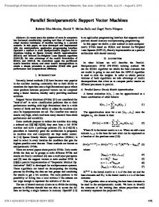
Fig. 1. Illustration of C-SVM and ECM learning scheme. In each level, the training set is divided into N/n subsets. This procedure is repeated consecutively until the target size n∗ of training set for support vectors is reached.
training set T[1,N ] = {(x1 , y1 ), . . . , (xN , yN )} of patterns xi with corresponding labels yi is divided into subsets of size n, i.e., T[j,k] = {(xj , yj ), . . . , (xk , yk )} (3) with xj , . . . , xk ∈ Rd and yj , . . . , yk ∈ {−1, 1}. On the first training set T[1,n] , the SVM parameters (kernel type, bandwidth parameter, regularization parameters) are chosen with grid search and cross-validation that are subject to the complete SVM parameter setup. This optimal parameter set κ∗ is used for all SVMs. Each SVM returns the support vectors as learning result. In each iteration, the training set is reduced to the corresponding set of support vectors. This process is stopped, when the final
Fig. 2. Comparison of SVM training result to training with support vectors, and the corresponding results on subsets (1st and 2nd half of training set) and their support vectors. The experiment shows that the C-SVM decision boundary is identical with the SVM boundary learned on the original training set.
Figure 2 shows the behavior of a C-SVM with radial basis function (RBF) kernel that divides the training set of patterns from the XOR problem into two parts. Figure 2(a) shows the learning result of an SVM with RBF kernel. Figure 2(b) shows the learning result of an SVM trained with support vector sets from two SVMs, one trained on the first half of the original data set and one trained on the second half. The figures show that both SVM learn the same decision boundary on the XOR data set. C. Extreme Cascading Often, not all features are important to efficiently solve classification problems, some may be uncorrelated with the label or redundant. The reduction of the number of features to a relevant subset in supervised learning is a common approach in machine learning [13], [4]. Plastria et al. [10] have shown
13
that a proper choice of methods and number of dimensions can yield to a significant increase in classifier performance.
T → T ∪ support vector patterns xi ∈ R end for T = T 0 , T 0 = {} until |T | ≤ n∗ return T
Fig. 3.
40,1000,5000 10,1000,5000 40,3000,5000 7
0.91
0.95 accuracy
0.97
0.99
200 160 d
120 80
Pseudocode of ECM algorithm
the ECM approach. The ECM employs many parameters that can be tuned to define the complete ECM model, from DR choice and target dimensionality q to DR method parameters and SVM parameters like kernel type, bandwidth parameters, and regularization parameter C. The reduced training sets Tˆ[·,·] are each subject to SVM training. After the SVM training, the patterns xi ∈ Rd that correspond to the support vectors of ˆi + w ˆTx ˆ0 ) = 1, are the intermediate SVMs, i.e., with yi (w 0 collected in the support vector set T . III.
0.93
(a) PCA-ECMs, d = 100
time
7: 8: 9: 10: 11:
0
10,1000,10000
9
Require: training set T , n, n∗ 1: κ∗ ← cv / grid search on T[1,n] 2: repeat 3: for α = 1 to N/n − 1 do 4: select training set T[α·n,(α+1)·n] 5: reduce dimensionality Tˆ[α·n,(α+1)·n] 6: train SVM on Tˆ[α·n,(α+1)·n] with κ∗ 0
40,1000,10000
11
time
The extreme cascade model we propose in this work combines cascading with dimensionality reduction. Each training subset is subject to a DR preprocessing resulting in reduced ˆ j,...,k ∈ Rq . subsets Tˆ[j,k] = {(ˆ xj , yj ), . . . , (ˆ xk , yk )} with x As the SVM training time also depends on the pattern dimensionality, the reduction to values q