Learning of Form Models from Exemplars Petra Perner and Silke Jänichen Institute of Computer Vision and applied Computer Sciences, IBaI, Körnerstr. 10, 04107 Leipzig
[email protected], www.ibai-institut.de
Abstract. Model-based image recognition requires a general model of the object that should be detected in an image. In many applications such models are not known a-priori instead of they must be learnt from examples. Real world applications such as the recognition of biological objects in images cannot be solved by one general model but a lot of different models are necessary in order to handle the natural variations of the appearance of the objects of a certain class. Therefore we are talking about case-based object recognition. In this paper we describe how the shape of an object can be extracted from images and input into a case description. These acquired number of cases we mine for more general shapes so that at the end a case base of shapes can be constructed and applied for case-based object recognition. Keywords: Annotation, Case Mining, Case-Based Object Recognition
1 Introduction Model-based object recognition is used to detect objects of interest on a complex background where thresholding-based image segmentation methods fail. The basis for such a recognition method is a good model of the object that should be recognized. Usually this method is applied for applications where the general appearance of the object is known or can be directly extracted from the image content. New applications such as biomedical applications require object recognition methods for segmentation but the object of interest is of great variation in appearance and cannot be modeled by a single model. A set of cases is necessary which describes the variation in appearance of the object on different abstraction levels so that it is possible to detect an object with a sufficient high recognition score. That is the point where case-based object recognition comes in charge. Such a method is based on a casebase filled up with different appearance cases of the objects of one class. A case is comprised of the contour points of an object and the case ID. The recognition is done by retrieving similar cases from the case base and matching these cases against the image. Objects whose pixel points match the case points with a high recognition score are marked in the actual image. Related work is described in Section 2. The image material used for this study is presented in Section 3. We describe how image information can be extracted from an image and mapped into a case description in Section 4. In order to learn groups of shapes that can be generalized by a more general shape we pair-wise align and rescale the shapes and calculate the similarity between the shape instances, see Section 5.
Based on the pair-wise similarity values we cluster the shape instances into groups and calculate prototypes for each group (see Section 6). These prototypes are then stored into the case base of the case-based object recognition system [26] and they are used for object recognition in new images. Results on the acquisition and learning process are given in Section 7. Finally we give conclusions in Section 8. The presented methods are implemented in our program named CACM Version 1.0.
2 Related Work The acquisition of object shapes from real images is still an essential problem of image segmentation. For the automated image segmentation often low-level methods, such as edge detection [2] and region growing [3], [4], are used to extract the outline of objects from an image. Low-level methods yield to good results if the objects have conspicuous boundaries and are not occluded. In the case of complex backgrounds and occluded or noisy objects, the shape acquisition may result in strong distorted and incorrect exemplars. Therefore segmentation is often performed manually at the cost of a very subjective, time-consuming procedure. Landmark coordinates [5], [6], [7], [8] can be assigned by an expert to some biologically significant points of an organism. If there are objects with an absence of anatomical landmarks, it is a common procedure to determine landmark points according to the defined mathematical or geometrical properties of the objects. However in some applications it is impossible or insufficient to describe the shape of an object only by means of these landmarks because important characteristics of the shape might be lost. To increase the total of landmarks it is usual to trace the complete outline of an object manually and subsequently determine corresponding points on each shape [10]. Semiautomatic approaches were developed [11], [12] for interactive image segmentation. These approaches use live-wire segmentation algorithms which are based on a graph search to locate mathematically optimal boundaries in the image. If the user moves the mouse cursor in the proximity of an object edge, the labeled outline is automatically adjusted to the boundary. Based on an acquired set of shape instances it is usually desirable to describe and compare deformations and distances between these shapes. The problems of shape spaces and distances have been intensively studied by Kendall [5] and Bookstein [6] in a statistical theory of shape. They assume that point correspondences between two sets of landmarks are already known. However at the beginning of many applications this condition is not hold and various approaches are made to determine corresponding points for the automated generation of statistical shape models. Hill et al. [10] presented a framework for the automated landmark identification on a set of two-dimensional, polygonal shapes. Their algorithm determines corresponding landmarks based on the arc-path length of the shapes on condition that the exemplars are out of the same object class and have similar contour lengths. Bookstein [13] applied landmark methods to continuous contours represented as thin-plate splines, but his approach is not completely automatic. The Softassign Procrustes Matching algorithm [15] solves the correspondence problem using deterministic annealing. This algorithm works robust with respect to outlier identification and noise, but is it also a
computationally-expensive procedure. Belongie et al. [14] found correspondences between points on the basis of the shape context descriptor. Latecki et al. [17] used a tangent space representation of shapes to determine correspondences of visually significant parts and to define a shape similarity measure. Another method was presented by Mokhtarian et al. [18] who calculate a similarity measure between two exemplars based on their maxima in the curvature scale-space. The analysis of these feature-based shape representations is problematic in cases of noisy or distorted cases.
3 Material used for this Study The materials we used for our study are fungal strains that are naturally 3-D objects but that are acquired in a 2-D image. These objects have a great variance in the appearance of the shape of the object because of their nature and the imaging constraints. Six fungal strains representing species with different spore types were used for the study. Table 1 shows exemplary one of the acquired images for each fungal strain. Table 1. Images of Six Different Fungi Strains
Alternaria Alternata Aspergillus Niger
Rhizopus Stolonifer
Scopulariopsis Brevicaulis
Wallenia Sebi
Ulocladium Botrytis
The strains were obtained from the fungal stock collection of the Institute of Microbiology, University of Jena/ Germany and from the culture collection of JenaBios GmbH. All strains were cultured in Petri dishes on 2 % malt extract agar (Merck) at 24°C in an incubation chamber for at least 14 days. For microscopy fungal spores were scrapped off from the agar surface and placed on a microscopic slide in a drop of lactic acid. Naturally hyaline spores were additionally stained with lactophenol cotton blue (Merck). A database of images from the spores of these species was produced.
4 Acquisition of Shape Cases We are considering the contour of an object S but not the appearance of the object inside the contour. Therefore we want to elicitate from the real image the object shape S C represented by a set of n SC boundary points si (x , y ) , i = 1,2 ,K nS C . We obtain the set of boundary pixels by implementing into our program a function that allows the user to mark the contour S C of an object S by moving the mouse cursor of the computer or by moving an electronic pen over a digitizer tablet. Notice that the sampled points are not required to be landmark coordinates or curvature extrema. The user starts labeling the contour S C of object S at an arbitrary pixel si (x , y ) ,
i = 1,2 ,K , j ,K n SC of the contour S C . After having traced the complete object the
labeling ends at a pixel s j (x , y ) in the 8-neighbourhood of si (x , y ) . To obtain the complete set S C of all boundary pixels we need to ensure that the contour is closed
which means s j (x , y ) is a direct neighbor of s i (x , y ) . Therefore we insert missing
boundary pixels using the Bresenham [20] procedure. Figure 1 presents a screenshot from our program CACM with three labeled shapes of the strain Ulocladium Botrytis with their coordinates on the right side of the screenshot.
Fig. 1. Labeled and Approximated Shapes with Coordinates
It might be very difficult to exactly determine or meet every boundary pixel of an object when manually labeling the contour of an object. The quantization of a continuous image constitutes a reduction in resolution which causes considerable image distortion (Moiré effect). Furthermore the contour of an object in a digitized image may be blurred which means the contour is extended over a set of pixels with decreasing grey values. In fact image digitization and human imprecision always implies small error rates in the object shapes. Therefore in the next step our intension is to introduce into the program procedures that help the user to find the right boundary of an object and that speed up the labeling process. As a result of the labeling process we obtain the set S C of nSC ordered, connected points that describes the boundary of the object S . Having labeled the contour S C of the object S its boundary pixels are still defined by their absolute position in the 2-D
matrix of the original image. In order to describe and compare the shapes of objects it is useful to specify a common coordinate system that is invariant under translation and scale. Therefore we transform the contour such that the centroid is at the origin and the maximum distance of the contour points from the origin is one. In a following approximation of the contour we reduce this set of pixels to a sufficiently large set of pixels that will speed up the succeeding computation time of the alignment and clustering process. The number of the pixels in this set will be influenced by the chosen order of the polygon and the allowed approximation error. For the polygonal approximation we used the approach based on the area/length ratio presented by Wall and Daniellson [21], because it is a very fast and simple algorithm without timeconsuming mathematic operations.
5 Shape Alignment and Similarity Calculation
5.1. Theory of Procrustes Alignment The aim of the alignment process is to compare the shapes of two objects in order to define a measure of similarity between them. Consider two shape instances P and O defined by the point-sets pi ∈ R 2 , i = 1,2 ,...N 1 and o j ∈ R 2 , j = 1,2 ,...N 2 respectively. The basic task of aligning two shapes consists of transforming one of them (say P ) so that it fits in some optimal way the other one (say O ). Generally the shape instance P = {pi ( x , y )}i=1...N is said to be aligned to the shape instance
{
}j =1...N
O = o j (x , y )
1
2
if a distance d min ( P ,O ) between the two shapes can not be
decreased by applying a transformation ψ to P . Various alignment approaches are known [16], [24], [2], [25]. They differ in the kind of mapping (similarity [2], rigid [9], affine [10]) and the chosen similarity measure [1]. For the similarity measure between P and O we use Procrustes distance [22]:
d ( P ,O ) =
N PO
∑ i =1
( pi − µ P ) − R(θ ) (oi − µO ) σP
2
(1)
σO
where R(θ ) is the rotation matrix, µ P and µO are the centroids of the object P and O respectively, σ P and σ O are the sums of squared distances of each point-set from the centroids and N PO is the number of point correspondences between the point-sets P and O . Thus the point correspondences are required for calculating the Procrustes distance. Generally this method is applied to centered shape instances represented by sets of landmark coordinates. Each of these shapes is rescaled so that the sum of squared distances of all landmarks to the centroid is identical (σ P = σ O ) . Then it is possible to compute a similarity transformation based on these centred pre-shapes. Finally the full Procrustes mean shape and Procrustes residuals [7] can be evaluated.
5.2. Our Approach to Shape Alignment We are considering a set of acquired shape exemplars where differences in the translation and the scale were already eliminated. To compare the shape of two instances P and O we still have to eliminate differences in the rotation. The measure of similarity between these two shape instances is based on the Procrustes distance. As it can be seen from equation (1) the Procrustes distance requires the knowledge of point correspondences between the shapes P and O . Therefore we are confronted with the following problems: 1. In our application we use the manually labeled set of contour points instead of a predefined number of landmark coordinates. Therefore we can not guarantee that all shape instances are defined by an identical number of contour points. 2. The point correspondences between the two shapes instances P and O are completely unknown. 3. We have no information about point outliers. Correspondences between two shapes were established based on the minimum mean alignment error of all possible positions. For every pair of points pi ,o j ∈ P × O we calculate the similarity transformation ψ ij that aligns these two
{
}
points pi and o j . The transformation ψ ij is applied to all points in P to obtain the transformed shape instance P' which is defined by the point-set p' k ∈ R 2 , k = 1,2 ,...N 1 . For every point p' k we define the nearest neighbour NN ( p' k ) in O as the point correspondence of p' k . Note that we do not enforce one-to-one point correspondences. One point in O can have more than one point correspondences or even not a single point correspondence in P . The sum of squared distances d ( P' ,O ) between every pair of point correspondents is calculated. In addition to that we define 1 the quantity d ( P' ,O ) as the mean alignment error ε ( P' ,O ) : N1
ε (P' ,O ) =
1 d (P' ,O ) N1
(2)
with
d (P' ,O ) =
N1
∑ ( p'
k − NN
( p' k ))2
(3)
k =1
If the distance d (P' ,O ) is smaller then all earlier calculated distances d min (P ,O )
is set to d (P' ,O ) , ε min (P ,O ) is set to ε (P' ,O ) , and ψ min is set to ψ ij . After having
{
}
iteratively aligned every possible pair of points pi ,o j ∈ P × O we may estimate the similarity between the shape instances P and O based on the value of the minimum mean alignment error ε min (P ,O ) . To ensure that our final measure of similarity
SCORE (P ,O ) ranges from 0 to 1 we normalize the measure ε min (P ,O ) to a
predefined maximum distance Tmax : SCORE (P ,O ) = 1 −
ε min (P ,O )
(4)
Tmax
If ε min (P ,O ) = 0 then the shape instance P is identical with shape instance O and the similarity measure SCORE (P ,O ) between these two shapes is 1 . With an increasing value of ε min (P ,O ) the shape instance P is less similar to shape instance O . If ε min (P ,O ) > Tmax then the term
ε min (P ,O ) Tmax
is automatically set to value one.
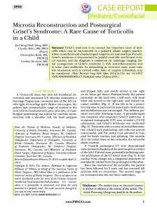
It is obvious that the constant Tmax has a direct influence to the value of the resulting score. The parameter Tmax can be defined by the user in the setting dialog of our program CACM. For our calculations we set Tmax to 35% of the mean distance of all contour points to the centroid. Our investigations showed that this value leads to good results. Figure 2 shows pair-wise aligned shapes and the calculated similarity scores. It can be seen that in case of identity the shapes are superposed. If the similarity score is less than one, we can see a deviation of the two shapes.
SCORE = 1 [identical]
SCORE = 0.9129 [nearly identical]
SCORE = 0.801 [similar]
SCORE = 0.5123 [neutral]
Fig. 2. Aligned Shape Instances of Strain Ulocladium Botrytis with Corresponding Similarity Measures
6 Clustering and Prototype Calculation The alignment of every possible pair of objects in our database leads us to N × N pair-wise dissimilarity measures between N exemplars. These distances can be collected in a dissimilarity matrix where each row and each column corresponds to an instance of our dataset. The dissimilarity measure SCORE (P ,O ) between shape instance P and shape instance O will be entered into the cell where the row of P and the column of O intersect. This results in a symmetric square matrix with diagonal elements equal to value zero since the dissimilarity measure between an instance and itself is zero.
This matrix is the input for the hierarchical cluster analysis [23]. After having investigated different hierarchical clustering methods we chose the single linkage method where two instances are merged together on the minimum distance between the two most similar instances of differing clusters.
Fig. 3. Clustering of Eight Instances of Strain Ulocaldium Botrytis Using Single Linkage with Resulting Prototypes at two Different Cut-Points (Vertical Red-Dotted Lines)
The result of the hierarchical cluster analysis can be graphically represented by a dendogram. The dendogram for eight shape instances of strain Ulocladium Botrytis is exemplary shown in Figure 3. The dendogram shows the distances between all instances. The merging of objects into clusters is done with increasing distances (from left to right) until all instances are combined in only one cluster. In the dendogram we marked two exemplary cut-points at different distances. A cut-point is a virtual vertical line in the dendogram. The horizontal position of this line marks the distance at which the individuals were split into several clusters. Therefore the distance of the cut-point has a direct influence on the resulting number of clusters and the number of prototypes. As smaller the distance is as more groups are created. That means the prototypes are more specialized which will result in matches with higher scores. As higher the chosen value for the dissimilarity is as fewer models have to be created. That means the cases are more general and the permissible distance between objects inside a cluster is higher. In general this will result to matches with lower scores. We have divided our set of N shape instances {P1 , P2 ,K PN } into k clusters
C1 , C2 ,K Ck . Each cluster Ci , i = 1,2 ,K k consists of a subset of ni shape cases. For each cluster we need to compute a prototype µˆ that will be the representative of the cluster. The full Procrustes estimate [7] of the mean shape is obtained by
2 minimizing (over µˆ ) the sum of squared full Procrustes distances d f from each
instance Pj , j = 1,2 ,K ni to an unknown unit size mean configuration µˆ , i.e. ni
[µˆ ] = arg inf ∑ d f (Pj , µˆ )² µˆ
(5)
j =1
In our approach we compared the similarity measures of all shape instances P1 , P2 ,...Pj included in the same cluster Ci , i = 1,2 ,K k . As the prototype we chose
{
}
the median shape Pmedian (Ci ) of that cluster that is the shape instance which has the minimum distance to all other shape instances: ni
[µˆ ] = Pmedian (Ci ) = arg inf ∑ d (Pmedian , Pj )²
(6)
j =1
The main advantage of this solution is that the prototype represents a natural shape instance out of that cluster. An example of using a natural shape instance as the prototype of a cluster is shown in Figure 5. With our program CACM it is possible to calculate the prototypes at different cutpoints. Each prototype can be exported as an image, where the contour pixels are labeled by the grey level one and the background pixels are labeled by zero, and as a list of coordinates of the contour points.
7 Results We have tested out approach on six different airborne fungi spores. Some digitized sample images for the analyzed spores are presented in Table 1. We have labeled a total of 60 objects for each of the six fungi strains. In the following registration process we have aligned every single object with all objects of the same strain to calculate the pair-wise similarity values. As a result we obtain six dissimilarity matrices, one for each analyzed fungi strain. These matrices are the input for the following cluster analyses. The outcome of this process was a dendogram for each of the six fungi strains. Now we need to define a cut-point on each dendogram to obtain the groups of the shapes. As described earlier the choice of the right position for a cutpoint is a central issue and it directly influences the recognition performance. Taking the minimal and the maximal distance d min and d max in each cluster we can calculate a cut-point by: k=
d max − d min n
(7)
where k is the minimal allowed distance and n is the maximal possible number of clusters. Table 2 presents the resulting number of models for each class at these cut-points.
Table 2. Number of Resulting Models of each Class with Recognition Rate
Classes Alternaria Alternata Aspergillus Niger Rhizopus Stolonifer Scopulariopsis Brevicaulis Ulocladium Botrytis Wallenia Sebi
Cut-Point Number of Models 0,045 34 0,017 5 0,027 22 0,063 8 0,025 30 0,158 10
Recognition Rate 0,031 0,029 0,037 0,050 0,020 0,065
The prototypes of these clusters were used as cases for the recognition process. Figure 6 shows exemplary the resulting casebase for the class Rhizopus Stolonifer.
Fig. 4. Casebase of Models for Strain Rhizopus Stolonifer Representing the 16 Resulting Clusters
8 Conclusions The recognition of objects in images can be done based on a model-based recognition procedure. That requires to have a model from the objects which should be recognized. Natural objects have a great variation in shape that makes it not easy to specify a model by hand. Therefore it is necessary to have a computerized procedure that helps to acquire the model from the real objects. We have proposed a method for the acquisition of contour instances and learning of general shape models. We use Procrustes similarity measure for aligning and determining the similarity between different shapes. Based on the calculated similarity measure we create clusters of similar shapes by using single linkage method. The mean shape or the median of the cluster is calculated and taken as prototype of the cluster. The methods are implemented in the program CACM Version 1.0 which runs on a Windows PC. Further research will be to improve the information gathering procedure and to develop an incremental clustering procedure.
Acknowledgement The project “Development of methods and techniques for the image-acquisition and computer-aided analysis of biologically dangerous substances BIOGEFA” is
sponsored by the German Ministry of Economy BMWA under the grant number 16IN0147.
References 1. R.C. Veltkamp, Shape Matching: Similarity Measures and Algorithms, Shape Modelling International, pp. 188-197, 2001 2. A. Rangarajan, H. Chui and F.L. Bookstein, The Softassign Procrustes Matching Algorithm, Proc. Information Processing in Medical Imaging, pp. 29-42, 1997 3. M. Kass, A. Witkin, and D. Terzopoulos, Snakes: Active contour models, In 1st International Conference on Computer Vision, pp. 259-268, London, 1987 4. D.-C. Cheng, A. Schmidt-Trucksäss, K.-S. Cheng, H. Burkhardt, Using Snakes to Detect the Intimal and Aventitial Layers of the Common Carotid Artery Wall in Sonographic Images, Computer Methods and Programs in Biomedicine 67, pp. 27-37, 2002 5. D.G. Kendall, A Survey of the Statistical Theory of Shape, Statistical Science, Vol. 4, No. 2, pp. 87-120, 1989 6. F.L. Bookstein, Size and Shape Spaces for Landmark Data in Two Dimensions, Statistical Science, Vol. 1, No. 2, pp. 181-242, 1986 7. I.L.Dryden and K.V.Mardia, Statistical Shape Analysis, John Wiley & Sons Inc., 1998 8. T.F. Cootes and C.J. Taylor, A Mixture Model for Representing Shape Variation, Image and Vision Computing 17, No.8, pp. 567-574, 1999 9. J. Feldmar and N. Ayache, Rigid, Affine and Locally Affine Registration of Free-Form Surfaces, The International Journal of Computer Vision, Vol. 18, No. 3, pp. 99-119, 1996 10. A. Hill, C.J. Taylor and A.D. Brett, A Framework for Automatic Landmark Identification Using a New Method of Nonrigid Correspondence, IEEE Transactions on Pattern Analysis and Machine Intelligence, Vol. 22, No. 3, pp. 241-251, 2000 11. E.N. Mortensen and W.A. Barrett, Intelligent Scissors for Image Composition, In Computer Graphics Proceedings, pp. 191-198, 1995 12. T. Haenselmann and W. Effelsberg, Wavelet-Based Semi-Automatic Live-Wire Segmentation, Proceedings of the SPIE Human Vision and Electronic Imaging VII, Vol. 4662, pp. 260-269, 2003 13. F.L. Bookstein, Landmark Methods for Forms without Landmarks: Morphometrics of Group Differences in Outline Shape, Medical Image Analysis, Vol. 1, No. 3, pp. 225-244, 1997 14. S. Belongie, J. Malik and J. Puzicha, Shape Matching and Object Recognition Using Shape Contexts, IEEE Transactions on Pattern Analysis and Machine Intelligence, Vol. 24, No. 24, pp. 509-522, 2002 15. A. Rangarajan, H. Chui and F.L. Bookstein, The Softassign Procrustes Matching Algorithm, Proc. Information Processing in Medical Imaging, pp. 29-42, 1997 16. D. Huttenlocher, G. Klanderman and W. Rucklidge, Comparing Images Using the Hausdorff Distance, IEEE Trans. Pattern Analysis and Machine Intelligence, Vol. 15, No. 9, pp. 850-863, 1993 17. L.J. Latecki and R. Lakämper, Shape Similarity Measure Based on Correspondence of Visual Parts, IEEE Transactions on Pattern Analysis and Machine Intelligence, Vol. 22, No. 10, pp. 1185-1190, 2000 18. F. Mokhtarian, S. Abbasi and J. Kittler, Efficient and Robust Retrieval by Shape Content through Curvature Scale Space, In Proc. International Workshop on Image Databases and Multimedia Search, pp. 35-42, 1996 19. P Besl and N. McKay, A Method for Registration of 3D Shapes, IEEE Trans. Pattern Analysis and Machine Intelligence, Vol. 14, No. 2, pp. 239-256, 1992
20. M. Petrou and P. Bosdogianni, Image Processing – The Fundamentals, John Wiley & Sons Inc., 1999 21. K. Wall and P.-E. Daniellson, A Fast Sequential Method For Polygonal Approximation of Digitized Curves, Comput. Graph. Image Process. 28, pp. 220-227, 1984 22. S.R. Lele and J.T. Richtsmeier, An Invariant Approach to Statistical Analysis of Shapes, Chapman & Hall / CRC, 2001 23. P. Perner, Data Mining on Multimedia Data, Springer Verlag Berlin, 1998 24. H. Alt and L.J. Guibas, Discrete Geometric Shapes: Matching, Interpolation and Approximation, Handbook of Computational Geometry eds. J.-R.Sack and J. Urrutia, Elsevier Science Publishers B.V., pp. 121-153, 1996 25. S. Sclaroff and A. Pentland, Modal Matching for Correspondence and Recognition, IEEE Trans. Pattern Analysis and Machine Intelligence, Vol. 17, No. 6, pp. 545-561, 1995 26. P. Perner and A. Bühring, Case Based Object Recognition, ECCBR 2004, submitted