Case Based Reasoning as an Extension of Fault Dictionary Methods for Linear Electronic Analog Circuits Diagnosis C. Pous, J. Colomer, J. Mel´endez and J.L. de la Rosa Institut d’Inform´atica i Aplicacions Edifici P-4 - Campus de Montilivi, 17071 Girona, Catalonia, Spain
[email protected]
Abstract. Even though there are plenty of methods proposed for diagnosing analog electronic circuits, the most popular are the fault dictionary techniques. The proposal of this paper is to extend the fault dictionary towards a Case Based Reasoning system. The case base memory, and the retrieval, reuse, revise and retain tasks are described. Special attention to the learning process is taken. An application example on a biquadratic filter is shown. Key Words: Analog circuits, Case-Based Reasoning, Fault dictionaries, Learning
1
INTRODUCTION
Test and diagnosis techniques for digital circuits have been successfully developed and automated. But, this is not yet the situation for analog circuits [4]. There are plenty of proposals on the bibliography for analog circuits testing, although fault dictionaries are the most extended ones. Artificial Intelligence techniques (AI) had a poor role during the first years of circuits testing. But this last decade, AI techniques have been a major research topic. In [5] a good review of AI techniques applied to electronic circuits is shown. The paper proposes four approaches: Traditional, Model-Based , Machine Learning, Hybrid and other approaches. Fault dictionaries are included in the Model-Based approaches, while Case-Based Reasoning in the Machine Learning Approaches group. As fault dictionaries can not learn from new situations, this paper proposes a methodology to extend a fault dictionary to a CBR-system. It is straightforward to use the dictionary table as a case base only with slight modifications [10]. The proposed methodology performs the learning keeping new cases when necessary and forgetting noisy exemplars using an IB3-like algorithm. Next section gives a short introduction to fault dictionaries and their limitations. Section 3 proposes the CBR system construction methodology and its cycle. Section 4 shows the result obtained applying the method to a biquadratic filter. Some conclusions are given in the last section.
2
FAULT DICTIONARIES AND THEIR LIMITATIONS
Fault dictionaries are techniques completely based on quantitative calculations. Once the universe of faults to be detected is defined (Fault 1, Fault 2, ..., Fault m), selected measures are obtained from the simulation of the system for each considered fault and stored in a table. These values will be then compared with the measures obtained from the unknown faulty system. The comparison is typically performed by the neighborhood criterion, obtaining distances, minimizing certain indexes, and so on. A possible fault dictionary is the one based on the response to a saturated ramp input with a rise time trin and a saturation value VSAT [3]. A typical circuit response to this input has four parameters: Steady state (V est ), overshoot (SP), rising time (tr ) and delay time (td ). The main drawbacks of fault dictionary techniques are the lack in detection for the nonconsidered faults and the tolerances effect. Mainly, the pre-simulated faults will be detected and located. Tolerances produce deviations of the simulated measures of the universe of faults initially considered. These discrepancies can produce a wrong diagnosis. This fact can be easily tested by generating random faulty cases corresponding to a considered fault, but taking the components tolerance into account. Hence, using the Monte-Carlo algorithm, for example, a set of faulty cases for each considered fault while other components value stay in its tolerance range, is generated. The dictionary performance in this situation is worsen. Of course, storing more cases is going to improve the percentage of diagnosis successes, but it increases the dictionary size, as well. 3
THE CBR-SYSTEM
Case Based Reasoning is an approach to problem solving that is able to use specific knowledge of previous experiences [7]. CBR has normally four stages for new problems solving [1], that it is repeated for each new experience: Retrieve similar past situations, Reuse , Revise and Retain if it is necessary. 3.1
Case Base Memory
The case structure is chosen to be the same used in the fault dictionary techniques, simply introducing a slight difference on the label that contains information about the fault. The proposed structure is shown in Figure 1 [8]. One part of the case is directly related with the measures taken from the circuit at one or several nodes. They could be temporal, frequencial or static measures. This numeric part will be used to retrieve the most similar cases. The second part of the case contains information about the fault diagnosis. One field has the faulty component location (Compo); the second contains the characterization of the fault (% of deviation from its nominal value Devi); Case Num Case i
Meas. 1 M1i
Meas. 2 M2i
… …
Meas. n Mni
Class Class i
Measures. Numeric Part
Figure 1: Case Structure
Compo Compo i
Devi X%
Fault. Qualitative Part
Hierarchy Li.Mj
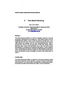
When there are deviations of the components smaller than the tolerance, the circuit is considered non faulty. This is known as the nominal case (Compo = N om). The third field (Hierarchy) has additional information about the component, to say, the level Li and the module Mj at which the component belongs to. Case base hierarchy is defined considering several levels depending on the circuit complexity [11]. Therefore, the diagnosis result could be more or less precise depending on the retrieved qualitative parts, according to Figure 2. The last level corresponds to the faulty component deviation. Next upper level is defined as the component level. At this point, the system will be only able to diagnose which component is wrong, but not the fault deviation. Also, it is possible that certain faults can only be located just at a certain module, but not deep inside it. So, going to upper levels, the circuit is divided in modules. The number of module levels depends on the circuit complexity. Circuit under test
MODULE LEVEL J
Module 1 faulty
. . .
MODULE LEVEL 1
Module 1 faulty
COMPONENT LEVEL
Module 2 faulty
Comp2 +20%
Comp1 Nom Comp1 - 20%
Comp1 +50%
Comp1 -50%
Comp2 Nom
Compo 3 faulty Comp2 -50%
Comp2 - 20% Comp2 +50%
Comp1 +20%
....
Module 3 faulty
Compo 2 faulty
Compo 1 faulty
DEVIATION LEVEL
Module 2 faulty
Module L2 faulty
....
Module L1 faulty
....
Compo N faulty
Comp3 -50%
Comp3 +20%
Comp3 Nom
Comp3 +50%
Comp3 - 20%
Figure 2: General Case diagnosis hierarchy
It is necessary to have certain knowledge on the circuit topology in order to build the case base hierarchy. For small circuits it can be done by inspection. For large circuits, the hierarchical decomposition approach proposed in [9] can be used. 3.2
Retrieve
It is necessary to define a metric and the number of cases k to retrieve from the case base (K-NN). Since the proposed CBR-system uses measures as data, the attributes are numeric and continuous. Therefore, among all possible distance functions, the normalized Euclidean weighted distance has been chosen. Attributes Normalization is necessary because of their different order of magnitude. Each of the k retrieved instances has an associated weight depending on its distance to the input vector. The weight is 1 when the distance is 0 and decreases as the distance grows larger. The way in which the weight decreases as the distance grows depends on which kernel function is used [12]. The number of cases, k, is an small odd number. In general, the more noisy is the data, the greater the optimal value of k.
3.3
Reuse
Once the k − nearest cases are extracted, they are used to propose a possible diagnosis. The proposal is to use the qualitative part of the extracted cases to derive a possible solution. Several situations can be given. If the Compo field of all the k extracted cases is the same, then the proposed solution is compound by the measures of the new case, the Compo field of anyone of them and the average deviation of the extracted cases in the field Devi and the same module Mi and level Lj . If Compo is different, the proposed solution will have a Compo made up with the different components, and each of them with its corresponding deviation in Devi. Hierarchy will contain the common module Mn or several if different, and the first common level Lm . The case adaption is completely done in the reuse task. It uses the past case solution instead of the past method that constructed the solution (transformational reuse) [1]. 3.4
Revise and Retain
Once the solution to the new presented case is proposed, it has to be revised. If the solution is considered right and accurate enough, it is not necessary to retain the new case. On the other hand, if it is considered wrong or with poor accuracy, the new case will be kept in the case memory. The revision analyzes how the cases that constitute the adapted solution are performing the diagnosis. There are 8 possible situations that are given in Figure 3 NE W C A SE
1 A re t he k
C om po fields
YE S
E Q U A LS ?
NO
A nd E Q U A L t o t he NE W ?
YE S
Is D ev i in t he m argin?
YE S
NO
NO
2
D ROP4
C om plet ely w rong. D ROP4
8
NO
E Q UA L t o t he N O M IN A L?
A ny one E Q UA L t o t he N E W ?
D iagnosis OK . D oNOT IN T R O D U C E
NO
D oNOT IN T R O D U C E
3
YE S
YE S
N ot D E T E C T A B LE . D ROP4
4
5 Is D ev i in t he m argin?
NO
D ROP4
NO YE S O K . D iagnosis is t he first common modu le
W eight O K > W eight w rong
YE S
It t ends t o perform incorreect ly . D ROP4 D iagnosis OK . NO T in t rodu ced
7
6
Figure 3: Decision flow diagram
The algorithm starts comparing the Compo of the retrieved cases to the Compo of the new case. If there is a coincidence, it carries on analyzing the Devi. Decisions 1 and 6 do not need
to introduce the new case because the adapted solution is satisfactory locating and identifying the fault. On the other hand, decision 3 accounts for a new case completely surrounded by faults belonging to other component. The introduction of this case, although necessary for its own right diagnosis, it is going to spoil its neighbors solution. Hence, it is not introduced. Case 4 correspond to a situation where the new case it is not distinguishable from the nominal. So, the fault could not be detected if it is not introduced. Decisions 5 and 7 represent the new cases with the k extracted neighbors with at least one of them with the same Compo. When no one of the k neighbors Compo matches the new case, it is a decision 8. In order to keep new cases on the case base, the DROP4 (Decremental Reduction by Optimization Procedure, version 4) is used [12]. Then, after taking the decision that a new case should be stored, the DROP4 algorithm is run. According to this algorithm, if this case is not going to disturb other cases diagnosis it will be finally introduced. 3.5
Forgetting noisy exemplars
When the case base size grows, there is a point where a degradation on the CBR-system performance is produced. The reason why is that there are previously kept cases that are performing worse when diagnosing. This is known as the utility problem. In order to reduce this factor, a maintenance of the case base memory is proposed. It is very similar to the IB3 algorithm given in [2], but only used for removal purposes. When the performance of a particular case drops below a certain established value with a certain confidence index, the case is considered to be spoiling the diagnosis and it will be deleted. The following section shows the results obtained by applying the method to a biquadratic filter. 4
RESULTS ON A REAL CIRCUIT
The proposed circuit to test is a biquadratic filter extensively used as a benchmark [6], [3]. It is a low-pass filter, allowing the pass of frequencies from DC to some certain desired frequency. It can be used itself or as part of the leap-frog filter. It is useful in audio and multi-media applications. The structure of the biquadratic filter is shown in Figure 4, with the component values R1=R6=2.7K, R2=1K, R3=10K, R4=1.5K, R5=12K, C1=C2=10nF. A tolerance of 10% is considered as normal for each component. Therefore, a component is considered faulty when it has a deviation greater than 10% from its nominal value. Module 1
R4
R6 C1
C2 Vi
R1 1
- V2 2 +
R5 R2 3
+
Module 2
V4 R3 4
5
+
V0
Module 3
Figure 4: Biquadratic filter under test
The circuit is linear and only parametric faults on the passive components are taken into account.
Consider for the fault dictionary construction that deviations of ±20% and ±50% for each component compound the universe of faults. Also, lets take the saturated ramp input with values tr = 100 µsec and VSAT = 1V as the fault dictionary method selected. The simulated measures at the output V0 produce a dictionary with 33 cases (32 faults + nominal). The faults for R2 , R3 and C1 are grouped because they produce exactly the same measures, forming an ambiguity group. The biquadratic filter is a small circuit that can be divided in 3 blocks by inspection, (M1, M2, M3), belonging to the same hierarchy level L1. M1 contains components R1, C2, R4 and R6; R2 and C1 belong to module M2; Module M3 is built up by devices R3 and R5. Therefore, component R1 belongs to level L1 and module M1, while component R5 belongs to the same level but to module M3. Hence, a case corresponding to fault at R5 with a deviation of -43%, using the measures derived from the saturated ramp method has the appearance of Figure 5. Case Num Case i
SP SPi
Td Tdi
Tr Tri
Vest Vesti
Class 20
Compo R5
Measures. Numeric Part
Devi -43%
Hierarchy L1.M3
Fault. Qualitative Part
Figure 5: Case Structure for the fault R1-43%
Let’s see some examples corresponding to a different type of decision on the biquadratic filter. A value of k = 3 has shown the best results for the proposed CBR system applied to the biquadratic filter example. An exponential distance-weighting kernel with a minimum value of wk = 0.2 for the k neighbor is used. Consider the results given in Table 1, where the measures are normalized. The 3 neighbors are all corresponding to Compo R 1 , the same Table 1: Case of a type 1 decision New case Neighbor 1 Neighbor 2 Neighbor 3
SP 0.5099 0.5411 0.5162 0.5546
td 0.5152 0.4242 0.4545 0.4545
tr 2.2353 2.2059 2.2353 2.2353
Vest 1.3024 1.2593 1.1525 1.0466
Compo R1 R1 R1 R1
Devi -54.6410 -54.5577 -50.00 -43.1893
Weight 0.5167 0.3765 0.2000
Compo field as the new case. As proposed by the algorithm of subsection 3.4, the average deviation should be obtained and compared to the new case. The average deviation of the 3 neighbors is Devi = −49.25%, that comparing with the deviation of the new case gives an error estimation of 9.86%. Since the error is less than 10%, the case is supposed to be correctly estimated, and therefore it is not necessary to introduce it in the case base. On the other hand, consider the results given in Table 2. Compo of the retrieved cases is Compo R 1 Table 2: Case of a type 2 decision New case Neighbor 1 Neighbor 2 Neighbor 3
SP 0.5487 0.4694 0.5598 0.5537
td 0.4545 0.5152 0.4545 0.3333
tr 2.2353 2.2647 2.2059 2.2059
Vest 0.4600 0.4918 0.5647 1.3462
Compo R1 R1 R1 R1
Devi 28.0632 13.7863 0 -57.877
Weight 0.8224 0.8216 0.2000
for all of them, and equal to the Compo of the new case. But, the deviation calculated as the median of the deviation of retrieved cases is −14.69%, that is far from being 28.0632%. The fault is located but not correctly identified. This is the situation of type 2 decision from the proposed algorithm. Hence, the case will be introduced if it does not disturb. Similar tables can be obtained for the other possible situations.
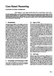
Figure 6 demonstrates how the process is learning while training. It has been obtained for 150 training sets randomly sorted and taking a confidence index of 0.9. Each training set is compound by 10 faults for each component considering deviations of ±70% randomly generated by means of the Monte-Carlo algorithm (a total of 80 new cases per train). Precision Success
Component Success 50 Percentage
Percentage
40
30
20
40 30 20
10
0
50 100 number of trainings
10
150
0
Wrong
150
Success with certain overlap 60 Percentage
40 Percentage
50 100 number of trainings
30 20
40
20 10 0
100 50 number of trainings
0
150
Total success
150
300 Number of cases
Percentage
50 100 number of trainings Data base dimension
100 90 80 70 60
0
0
50 100 number of trainings
150
200
100
0
50 100 number of trainings
150
Figure 6: Analysis sorting the train sets
Precision success stands for the cases that are diagnosed correctly (component and deviation with an error < 10%). On the other hand, Component success represent the percentage of cases that are correct only locating the component (deviation with an error > 10%). Cases with neither component nor deviation are correct are considered in the Figure 6 as Wrong. Success with overlap contains the percentage of faults that provides the correct diagnosis only at the faulty module. The sum of all these types of successes is given in Figure 6 by Total success. At last, the Data base size during training is shown in the last graphic of the same figure. The first value displayed in each graphic of Figure 6 corresponds to the diagnostic values obtained by the classic dictionary (Precision success:14.12%, component success:43%,wrong: 38.5%, success with overlap: 4.37%, total success: 61.5%, data base size: 25). At the beginning, the total of correct cases increases abruptly. This fact is due to take multiple cases instead of one as a neighbor in the diagnosis. Therefore, it is more probable to extract the correct class between them, but overlapped with the other neighbors. As the training advances, the case base is substituting component and module success diagnosis by increasing the average of precision diagnosis. On the other hand, another important factor to observe is that the number of cases continuously increase. Observe that the system classifies correctly (including the deviation), almost 40% of the tested new cases. If the situations in which at least the component or its corresponding module is diagnosed correctly, almost 90% of the new tested cases are properly located and identified. These percentages show that better results are obtained comparing with the fault dictionary. 5
CONCLUSIONS
A new methodology for building a CBR system for analog electronic circuits diagnosis has been developed. A fault dictionary technique has served as starting point for its development,
since it is the more extended technique and it is very simple to apply. The case base memory has cases with fields inherit from the fault dictionary technique. About the learning algorithm, a mixture of DROP4 for adding and IB3 for deleting cases has been proposed. The method seems to work quite well. Of course taken more measures at other nodes will decrease the number of ambiguities and more faults will be distinguishable, as it will happen with the classical dictionaries or other studied methodologies. But comparing the success rate for the studied methods all of them in the same conditions (taking measures only at the output), the proposed CBR system presents a higher percentage of success identifying the parameter values. As it usually happens with the training processes, it is not clear the best order in which to present the new situations to the case base for learning. Results of the designed CBRsystem demonstrates that depending on the order of training the case base can learn faster, although the final results do not show extremely different outcome. This methodology have to be tested with other circuits, although the improvement on the diagnosis results is expected to be obtained. References [1] A. Aamodt and E. Plaza, ‘Case-based reasoning: Foundationalu issues, methodological variations and system approaches’, AI Communications, 39–59, (1994). [2] D. W. Aha, D. Kibler, and M. Albert, ‘Instance based learning algorithms’, Machine Learning., 6, 37–66, (1991). [3] A. Balivada, J. Chen, and J.A. Abraham, ‘Analog testing with time response parameters’, IEEE Design and Test of computers, 18–25, (Summer 1996). [4] A. Fanni, A. Giua, M. Marchesi, and A. Montisci, ‘A neural network diagnosis approach for analog circuits’, Applied Intelligence 2, 169–186, (1999). [5] B. Fenton, M. McGinnity, and L. Maguire, ‘Fault diagnosis of electronic systems using artificial intelligence’, IEEE Instrumentation and Measurement, 16–20, (September 2002). [6] B. Kaminska, K. Arabi, P. Goteti, J.L. Huertas, B. Kim, A. Rueda, and M. Soma, ‘Analog and mixed signal benchmark circuits. first release’, IEEE Mixed Signal Testing Technical Activity Committee ITC97, 183–190, (1997). [7] R. Lopez de Mantaras, , and E. Plaza, ‘Case-based reasoning: An overview’, AI Communications, 21–29, (1997). [8] C. Pous, J. Colomer, J. Melendez, and J.L. de la Rosa, ‘Case base management for analog circuits diagnosis improvement’, Proceedings of the 5th International Conference on Case-Based Reasoning ICCBR03, Case-Based Reasoning Research and Development(LNAI 2689), 437–451, (June 2003). [9] A. Sangiovanni-Vicentelli, L. Chen, and L.O. Chua, ‘An efficient heuristic cluster algorithm for tearing large-scale networks’, IEEE Transactions on Circuits and Systems, cas-24(12), 709–717, (December 1977). [10] J. W. Sheppard and W. R. Simpson, Research Perspectives and Case Studies in Systems Test and Diagnosis, volume 13 of Frontiers in Electronic Testing, Kluwer, September 1998. Chapter 5. Inducing Inference Models from Case Data.ISBN 0-7923-8263-3. [11] R. Voorakaranam, S. Chakrabarti, J. Hou, A. Gomes, S. Cherubal, and A. Chatterjee, ‘Hierarchical specification-driven analog fault modeling for efficient fault simulation and diagnosis’, International Test Conference, 903–912, (1997). [12] D. Wilson and T. Martinez, ‘Reduction techniques for instance-based learning algorithms’, Machine Learning, 38(3), 257–286, (2000).