CASSCF Calculations in ORCA: A tutorial Introduction

1

CASSCF Calculations in ORCA: A tutorial Introduction D. Aravena, M. Atanasov, V. G. Chilkuri, Y. Guo, J. Jung, D. Maganas, B. Mondal, I. Schapiro, K. Sivalingam, S. Ye and F. Neese

Contents 1

Introduction .................................................................................................................................................... 2

2

The [Cr(NH3)6]3+ complex – a standard run .................................................................................... 4 2.1

Organization of the Calculation: Preliminary Chemical Considerations ................... 4

2.2

Initial 3d CAS(3,5)................................................................................................................................ 5

2.3

Including ligand orbitals CAS(7,7) ............................................................................................... 7

2.4

Including a second d-shell CAS(7,12) ......................................................................................... 8

2.5

Reading the wave function ........................................................................................................... 11

2.6

NEVPT2 CAS(7,12) ........................................................................................................................... 12

3

[Cr(NH3)6]3+ complex - extracting ligand field parameters. ................................................. 14

4

[CrCl6]3- model complex - CASSCF for larger active spaces................................................... 18

5

A comment on using ANO basis sets ................................................................................................ 21

6 [FeIV(O)(TMC)(MeCN)]2+ - covalent metal-ligand interactions and the computation of MCD / Mössbauer .......................................................................................................................................... 23

7

8

6.1

Calculation of MCD spectra and Quadrupole splitting .................................................... 30

6.2

Mössbauer Parameters .................................................................................................................. 33

[Co(SH)4]2- - Optical and Magnetic properties ............................................................................. 34 7.1

Electronic Structure ......................................................................................................................... 34

7.2

Setting up the CASSCF/NEVPT2 calculation ........................................................................ 35

7.3

Optical spectra .................................................................................................................................... 37

7.4

G-tensor ................................................................................................................................................. 39

7.5

D-tensor ................................................................................................................................................. 41

Cu-dimer J-Couplings with NEVPT2, DLPNO-NEVPT2 and MRCI ...................................... 42 8.1

CASSCF(2,2) and NEVPT2 ............................................................................................................. 42

8.2

CASSCF(2,2) DDCI3 - the game changer ............................................................................... 44

8.3

RI approximation for CASSCF, NEVPT2, DLPNO-NEVPT2 and MRCI ...................... 46

8.4

CASSCF(18,10) and NEVPT2 ....................................................................................................... 48

8.5

Wave function Printing .................................................................................................................. 49

8.5.1

CASSCF and ICE ......................................................................................................................... 49

8.5.2

MRCI ............................................................................................................................................... 50

2 9 A comment about CASSCF calculations on heavier elements (lanthanide- and actinide-based systems) .................................................................................................................................. 51 9.1

Basis, RI-Basis and ECP .................................................................................................................. 51

9.2

Initial guess .......................................................................................................................................... 52

9.3

Additional features concerning CASSCF calculations on f-elements systems ..... 53

9.4 Example: Investigation of the spectroscopic and magnetic properties of the Cs2NaDyCl6 elpasolite ................................................................................................................................... 53 10 Fragment Derived Guess (orca_mergefrag) ................................................................................. 60 11 Manipulation of the ORCA GBW File (orbitals) ........................................................................... 62 12 p-Phenylenediamine (PPD) ground state - organic molecule ............................................. 64 13 Adenine spectra – using symmetry .................................................................................................. 68 14 NEVPT2-F12 – reaching the basis set limit ................................................................................... 72 15 Appendix [Cr(NH3)6]3+ - detailed walkthrough .......................................................................... 74 15.1

[Cr(NH3)6]3+ complex - a walk through tutorial guide................................................ 74

15.2

Organization of the Calculation: Preliminary Chemical Considerations ........... 74

15.3

Initial guess CASSCF .................................................................................................................... 76

15.4

State-Averaging as convergence aid.................................................................................... 80

15.5

Including ligand orbitals ........................................................................................................... 81

15.6

Including a second d-shell ........................................................................................................ 82

15.7

Basis set projection (increasing the basis set) ............................................................... 84

15.8

Calculating the ligand field spectrum ................................................................................. 86



1 Introduction The complete active space self-consistent field (CASSCF) theory is one of the most used and powerful methods for electronic structure calculations of transition metals. In contrast to widely used DFT methods, CASSCF is not a black box method because it requires the user to select a set of orbitals and electrons that constitutes the active space. Hence, the input for a CASSCF calculation is case-specific and requires some consideration from the user with respect to the computational setup. This tutorial is complementary to the section “running typical calculation” of the ORCA manual. The aim of this tutorial is to introduce possible strategies to carry out such CASSCF calculations on transition metal complexes. Here is a list of details to be considered: · Inclusion of all d-orbitals in the active space · Inclusion of the second d-shell in the active space · Addition of a few ligand orbitals in the active space · State-averaging of excited states and different spin multiplicities · Use of a large basis set · Use of an ANO basis set

3 · · · · · ·

Interpreting the wave function (CSFs and spin determinants) Ab initio ligand field analysis Property calculations (MCD, Mössbauer parameters, ZFS, g-tensor, ...) Inclusion of dynamic electron correlation (NEVPT2/MRCI) RI Approximation in CASSCF, NEVPT2 and MRCI Using point-group symmetry in ORCA

Before running a CASSCF calculation of a transition metal it is crucial to have some chemical intuition and a basic understanding of the electronic structure of the selected system. In the following sections, we will go step by step through a few examples and illustrate how one can approach all these considerations. By doing so, we explore several “initial guesses”, convergence strategies and interesting features of the CASSCF program. For more details on the available options and the general program usage we refer to the ORCA manual. Before diving into the practical examples, note that a converged CASSCF wave function is the starting point for a subsequent multireference calculation that takes into account dynamic electron correlation. Commonly applied multireference methods are multireference configuration interaction (MRCI) and multireference perturbation theory (MRPT). The internally contracted N-Electron valence state perturbation theory (NEVPT2) is often the first choice to include dynamical correlation. 1,2,3 The method is efficient and requires only one additional keyword to the CASSCF input: %casscf ... nevpt2 sc # for SC-NEVPT2, corresponds to “nevpt2 true” # in older version of ORCA (2.9 - 3.0.3) end

In previous version of ORCA, “NEVPT2” abbreviates the “strongly contracted” version of the NEVPT2 approach. Starting with ORCA 4.0, the PC-NEVPT2 approach in the canonical and in the DLPNO methodology is available.4 Since the employed wave function is fully internally contracted (FIC), we prefer to call the method FIC-NEVPT2. Details and input examples are discussed in Section 8. There we will also illustrate calculations with the orca_mrci module. Final notice: ORCA 4.0 has different frozen core settings compared to previous version. For transition metal complexes, the 3s and 3p orbitals are now correlated. They are quite important for the accurate energies and properties such as zero field splitting (ZFS).5

1 C. Angeli, R. Cimiraglia, and J.-P. Malrieu, Chem. Phys. Lett. 350, 297 (2001). 2 C. Angeli, R. Cimiraglia, S. Evangelisti, T. Leininger, and J.-P. Malrieu, J. Chem. Phys. 114, 10252 (2001). 3 C. Angeli, R. Cimiraglia, and J.-P. Malrieu, J. Chem. Phys. 117, 9138 (2002). 4 Y. Guo, K. Sivalingam, E.F. Valeev, and F. Neese, J. Chem. Phys. 144, 94111 (2016). 5 K. Pierloot, Q.M. Phung, and A. Domingo, J. Chem. Theory Comput. 13, 537 (2017).

4

2 The [Cr(NH3)6]3+ complex – a standard run

Quit often we are interested in the ligand field spectrum of a transition metal complex. As a simple example, we study a Cr(III) model complex. From elementary inorganic chemistry, we know that Cr(III) is a d3-system and hence, the three metal d-electrons are our primary focus. In later stage will explore various active spaces: · CAS(3,5) consisting of the five 3d metal orbitals. · CAS(7,7) includes two ligand orbitals. · CAS(7,12) extended to include the second d-shell. In this section, we demonstrate our standard approach to do such calculation. In the appendix we find a slower paced description of the same example with much more details on the selecting active orbitals/initial guess, state-averaging and basis-set projection.

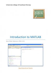
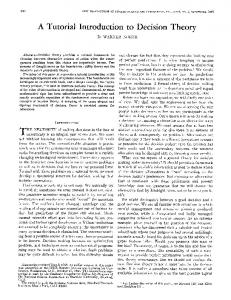
2.1 Organization of the Calculation: Preliminary Chemical Considerations As mentioned above, the central Cr3+ ion is a d3 system. Since the [Cr(NH3)6]3+ complex is very close to an octahedral coordination, we can expect the three metal t2g-based orbitals to be singly occupied and hence a 4A2g ground state arises. Each NH3 provides a single lone pair that can form a σ-bond with the central metal, but no π-bonds are possible. Hence, we only need the two ligand orbitals of eg-symmetry when we want to include the ligand orbitals in the active space. For Cr, Ammonia acts as a strong field ligand. If we are interested in the d-d excited states of the system, the Tanabe-Sugano diagram (Figure 25) tell us, that we expect 4T2g and two 4T1g excited states of the same multiplicity as the ground state.6 Since T-terms are triply orbitally degenerate, 10 roots need to be calculated to capture all spin allowed ligand field transitions. Of course, due to the presence of the hydrogens, the actual symmetry is not strictly octahedral, but we use Oh group notation nonetheless. According to the Tanabe-Sugano diagram, the next double states are derived from the free ion 2G term, which splits into the triply degenerate 2T2, 2T1, the doubly degenerate 2E terms and an 2A term. Thus, we need a total of nine doublet roots. 1

6 Derived from the 4F and 4P terms of the free ion.

5



Figure 1: Tanabe-Sugano diagram for d3 system in octahedral field

The initial geometry of the complex comes from a DFT geometry optimization, but it can also be based on the crystal structure with just the hydrogens optimized. # # # # *

This is a slightly smoothed DFT optimized geometry in internal coordinates. This helps keeping the orbitals clean, as the ligands will be placed on the coordinates. Any xyz coordinates would do too, just replace “int” by “xyz” and give Cartesian Coordination (in Angström) int 3 4 Cr 0 0 0 0 0 0 N 1 0 0 2.137 0 0 N 1 2 0 2.137 90 0 N 1 2 3 2.137 90 90 N 1 2 3 2.137 90 180 N 1 2 3 2.137 180 180 N 1 2 3 2.137 90 270 H 2 1 3 1.041 114 0 H 2 1 3 1.041 114 120 H 2 1 3 1.041 114 240 H 3 1 2 1.041 114 0 H 3 1 2 1.041 114 120 H 3 1 2 1.041 114 240 H 4 1 2 1.041 114 315 H 4 1 2 1.041 114 195 H 4 1 2 1.041 114 75 H 5 1 2 1.041 114 0 H 5 1 2 1.041 114 120 H 5 1 2 1.041 114 240 H 6 1 4 1.041 114 270 H 6 1 4 1.041 114 30 H 6 1 4 1.041 114 150 H 7 1 2 1.041 114 45 H 7 1 2 1.041 114 165 H 7 1 2 1.041 114 285

*

It is advisable to align the molecule with respect to the coordinate axis e.g. in this example the nitrogen atoms should be along the x,y,z-axis. This merely simplifies the identification of the orbitals later on but has no influence on the mechanics of the calculation.

2.2 Initial 3d CAS(3,5) We start with the smallest active space that is just the 3d-metal orbitals. In later stages, we can use these converged calculations to further extend the active space. In general, this is a good strategy for TM complexes with mostly ionic interactions between metal and ligands, where the 3d-metal orbitals are strongly localized.

6 CASSCF calculations require the user to specify the number of active electron in active orbitals. The program automatically starts with the “PModel” (~diagonalized LDA DFT matrix) as initial guess. For many applications this is not a sufficient input as the active orbitals are not consciously chosen. For transition metal complexes the desired 3d-metal orbitals are often below HOMO-LUMO gap and hence do not automatically enter the active space. The “PAtom” guess gives good atomic orbitals, with an extended Hückel like ordering, which is a good idea for transition metal calculations as the desired metal 3d-orbitals are typically at the HOMO-LUMO gap and essentially of metal character. # # Initial CASCF on [Cr(NH3)6]3+ # # def2-TZVPP = triple zeta basis # RI-JK = use the RI-JK approximation for the Fock matrix # (not required – just used for more speed here) # def2/JK = auxiliary basis for the RI approximation (Fock and gradient integrals) # Conv = store integrals on disk (required for RIJK) # XYZFile = leave coordinates on disk (convenient later) # normalprint = slightly larger printing than default + includes Loewdin # population analysis. ! def2-TZVPP def2/JK RI-JK Conv XYZFile PATOM %casscf nel 3 # number of active electrons norb 5 # number of active orbitals mult 4,2 # multiplicity blocks nroots 10,9 # Roots per multiplicity blocks end * int 3 4 Cr 0 N 1 N 1 N 1 N 1 N 1 N 1 H 2 H 2 H 2 H 3 H 3 H 3 H 4 H 4 H 4 H 5 H 5 H 5 H 6 H 6 H 6 H 7 H 7 H 7 *

0 0 2 2 2 2 2 1 1 1 1 1 1 1 1 1 1 1 1 1 1 1 1 1 1

0 0 0 3 3 3 3 3 3 3 2 2 2 2 2 2 2 2 2 4 4 4 2 2 2

0 2.137 2.137 2.137 2.137 2.137 2.137 1.041 1.041 1.041 1.041 1.041 1.041 1.041 1.041 1.041 1.041 1.041 1.041 1.041 1.041 1.041 1.041 1.041 1.041

0 0 90 90 90 180 90 114 114 114 114 114 114 114 114 114 114 114 114 114 114 114 114 114 114

0 0 0 90 180 180 270 0 120 240 0 120 240 315 195 75 0 120 240 270 30 150 45 165 285

The above calculation the orbitals are state-averaged. In ORCA 4.0, the default stateaveraging sets equal weights for multiplicity blocks. The actual weights are also printing in the output before the first CASSCF iteration, when the CI is setup. In the following, the RI approximation is used to speed up the calculations. In Section 8.3, you will find more information on the accuracy of the RI approximation. The keyword “xyzfile” produce a xyz coordinate file on disk that we use in later inputs (cr_example1.xyz). The calculation converges in 8 iterations. The results are reported in Table 2 with the extended active spaces.

7

2.3 Including ligand orbitals CAS(7,7) In the second step, we improve the reference wave function by including the metalligand bonding orbitals in the active space. Having the bonding and anti-bonding orbitals should balance the active space. The orbitals are sorted by their energies. Hence, the desired orbitals may not be the highest doubly occupied orbitals. In fact, they are usually not. The highest ligand orbitals are typically non-bonding, whereas we are looking for bonding orbitals that are stabilized. Identifying these orbitals from the previous calculation requires looking at the orbital coefficients or better to visualize the molecular orbitals. In this example, the reduced Loewdin analysis printed at the end of the CAS(3,5) calculation is sufficient to identify the ligand orbitals.7 The ligand orbitals of interest are the bonding partners of the dz2 and dx2-y2 orbitals. In our example, we obtain:

0 0 0 1 1 1 1 2 2 2 2 3 3

Cr Cr Cr N N N N N N N N N N

s dz2 dx2y2 s pz px py s pz px py s pz

34 -1.02677 2.00000 -------0.0 0.0 25.2 0.7 0.0 17.0 0.0 0.7 0.0 0.0 17.0 0.0 0.0

35 -1.02677 2.00000 -------0.0 25.2 0.0 0.2 0.0 5.3 0.0 0.2 0.0 0.0 5.3 0.9 22.3

Hence, we need to use the “rotate” feature in order to bring the correct orbitals on top of the (formerly) doubly occupied space to include them in the active space of the next calculation. The previously converged CAS(3,5) orbitals are denoted as “cas_5.gbw”. Here is the ORCA input: # # Second step: include ligand orbitals # ! def2-TZVPP def2/JK RI-JK conv ! moread %moinp "cas_5.gbw" # orbitals from the CAS(3,5) calculation # The highest doubly occupied inactive orbitals are 37 and 38. %scf rotate {34,37,90} {35,38,90} end end %casscf nel 7 norb 7 mult 4,2 nroots 10,9 end * xyzfile 3 4 cr_example1.xyz #previously generated xyzfile

7 Identifying orbitals with the Loewdin analysis is bread and butter for CASSCF. A small parsing script that filters all metal dominating orbitals might be handy.

8 This calculation converges in 5 iterations. The resulting gbw-file is denoted as “cas_7.gbw”.

2.4 Including a second d-shell CAS(7,12) In some cases, including a second d-shell can be useful to make the wave function more flexible and obtain accurate results in conjunction with a subsequent second order multireference perturbation method such as CASPT2 or NEVPT2.8 Most often it is not necessary to include the entire second d-shell, but the ones that correspond to the occupied 3d-metal orbitals. To find the second d-shell, we use the keyword “extorbs doubleshell” in the converged CAS(7,7) calculation. Based on the composition of the highest active orbital, the program automatically identifies and produces a “second shell” in the vicinity of the active space. It is important that the highest active orbital indeed has largest contribution from the metal based d-orbital. For an active space consisting of 3d-metal orbitals the second shell consists of the 4d-metal orbitals. For an active space consisting of 4d-metal orbital, the second shell consists of 5d-metal orbitals and so on. Note that the option does not work in conjunction with symmetry (UseSym). The following input reads the converged CAS(7,7) orbitals and produces the second-d shell (orbitals 44-48) in the correct order. ! def2-TZVPP def2/JK RI-JK conv ! moread %moinp "cas_7.gbw" # orbitals from the cas(7,7) calculation %casscf nel 7 norb 7 mult 4 nroots 10 extorbs doubleshell # produce the double-shell above the actives. # all other virtuals are canonicalized end * xyzfile 3 4 cr_example1.xyz

As printed in the output, orbital nr.43 (highest active) is taken as reference and the double-shell is produced in the MO range 44-48. ---------

---- THE CAS-SCF GRADIENT HAS CONVERGED ------ FINALIZING ORBITALS ------ DOING ONE FINAL ITERATION FOR PRINTING ---Forming Natural Orbitals Canonicalize Internal Space SortedExt: Largest compononent of the highest active orbital (Nr. 43) on atom SortedExt: Double Shell Range 44 -> 48

0 Cr with l=2

We confirm the correctness by inspecting the Loewdin population analysis and visualizing the orbitals (see the next subsections). The associated gbw file is denoted as “cas_7_sorted.gbw” in the next step. 43

44

45

46

47

8 The second d-shell brings in a radial correlation effect that normally should be covered by the dynamical correlation treatment. However, second order perturbation theory with a contracted first-order interacting space is not flexible enough to provide this missing correlation. It is somewhat counter the philosophy of the CASSCF method (or MCSCF in general) to include dynamic correlation in the active space. However, it is common practice and hence described here.

9

0 0 0 0

Cr Cr Cr Cr

dxz dyz dx2y2 dxy

-0.57548 0.60166 -------49.4 49.4 0.0 0.0

0.26599 0.00000 -------0.0 0.0 0.0 90.4

0.26614 0.00000 -------45.2 45.2 0.0 0.0

0.26629 0.00000 -------45.2 45.2 0.0 0.0

0.77121 0.00000 -------0.0 0.0 69.3 0.0

Having generated a double-shell, we will setup the calculation for the extended active space. Since we start from an already converged CASSCF wave function, we may try the Newton-Raphson method (keyword “switchstep nr”) to obtain convergence here. The rate of convergence is higher with this method, but the radius of convergence is smaller. The program can use two different convergers specified with “orbstep” and “switchstep”. Far off from convergence “orbstep” is used. The SuperCI is good choice for large initial gradients. ORCA changes the converger to “Switchstep” when the calculation is close to convergence (||g|| < 0.02).9 The NR method is a safe pick for re-converging calculations that have already been converged with a slightly different active space or basis set. ! def2-TZVPP def2/JK RI-JK conv ! moread %moinp "cas7_sorted.gbw" # cas(7,7) orbitals with prepared virtual space. %casscf nel 7 norb 12 #3d + ligands + 4d orbitals mult 4 nroots 10 cistep accci # faster, more memory hungry algorithm for the CI step switchstep nr end * xyzfile 3 4 cr_example1.xyz

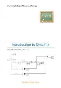
In many cases, switching to the computationally more demanding NR solver does not result in net time savings. In this example, the “switchstep NR” and the default converger perform equally well (4-6 iterations). For larger active spaces or many roots, the timings can be considerably improved using the “CIStep ACCCI” for the CI calculation. The method is absolutely equivalent to the default CI solver, but uses are more memory demanding algorithm. The final set of orbitals is denoted as “cas_12.gbw” in the next section. The orbitals and the occupation numbers from the converged calculation are shown below. They are ordered by increasing occupation number. You see an ideal shape and ordering of the orbitals, which makes the interpretation of the results very convenient. It is also a quality control for your calculation to ensure that you have arrived at the desired enlarged active space. Note that not all of the orbitals are perfectly aligned to the coordinating ligands. This is perfectly normal as some of the orbitals are degenerate and hence arbitrarily mixed.

9 controlled by the keyword “switchconv”

10



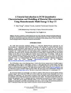
Figure 2: These two orbitals are the antibonding eg-counterparts in the second d-shell. Notice how large these orbitals are. If we would plot a radial cut, you would observe that they have a node, whereas the primary dorbitals do not have it. (isosurface value 0.05)



Figure 3: These three orbitals are the second d-shell counterparts of the nonbonding t 2g based metal orbitals.

Figure 4: These three orbitals are the nonbonding metal d-orbitals of t 2g origin.



Figure 5: These are the antibonding eg based orbitals in the primary metal d-based set.



11



Figure 6: These two orbitals are the essentially doubly occupied bonding counterpart of the metal eg-orbitals



2.5 Reading the wave function The actual weights are also printing in the output before the first CASSCF iteration, when the CI is setup. Let us look at some of the results of this calculation. After convergence, you find the definition of the wave function for each state: --------------------------------------------CAS-SCF STATES FOR BLOCK 1 MULT= 4 NROOTS=10 --------------------------------------------ROOT

ROOT

0: E= 0.96625 0.00458 0.00440 0.00439 0.00271 0.00271 1: E= 0.73142 0.23945 0.00410 0.00271

[ [ [ [ [ [ [ [ [ [

-1379.8845593013 Eh 0]: 221110000000 2552]: 111111100000 165]: 211111000000 1828]: 121110100000 809]: 201112000000 6660]: 021110200000 -1379.7943086004 Eh 2.456 eV 1]: 221101000000 9]: 221010100000 2]: 221100100000 1835]: 121101100000

...

The program then lists the main contributing configurations that are active space occupation patterns. For example, the ground state has a weight of 0.96625, which means that the lowest root is dominated to 96.6% by a single configuration (this number is the sum of the squares of the CI coefficients for all configuration state functions that belong to this configuration, e.g. the linearly independent spin couplings). This configuration has the active space occupation pattern 221110000000 which means the first active orbital is doubly occupied, the second doubly occupied as well, the next three orbitals are singly occupied and the remaining orbitals are empty. If you look at your orbitals (see above), you see that the first two are the ligand based bonding orbitals, the next three the metal t2g based orbitals, followed by the two metal eg based orbitals and the remaining ones are the second d-shell.10 ORCA by default uses natural orbitals for the active space. The metal eg based orbitals have a slightly higher occupancy due the presence of the ligand orbitals. 10 The number in square brackets is the number of the configuration in the configuration list and is irrelevant.

12 Note that ORCA employs configuration state functions. Occasionally one interested in the CI Coefficients or the representation in terms of spin determinants. This is possible with the keyword “PrintWF” and discussed in Section 8.5 in more detail. The program then prints the CASSCF transition energies: ----------------------------SA-CASSCF TRANSITION ENERGIES -----------------------------LOWEST ROOT (ROOT 0 ,MULT 4) =



STATE 1: 2: 3: 4: 5: 6: 7: 8: 9: 10: 11: 12: 13: 14: 15: 16: 17: 18:

ROOT MULT DE/a.u. 0 2 0.086665 1 2 0.086672 2 2 0.090109 3 2 0.090113 4 2 0.090115 1 4 0.090270 2 4 0.090279 3 4 0.090295 5 2 0.125745 6 2 0.125752 7 2 0.125760 4 4 0.128986 5 4 0.128987 6 4 0.129017 8 2 0.160764 7 4 0.202961 8 4 0.202968 9 4 0.202991

-1379.884565085 Eh -37548.568 eV DE/eV 2.358 2.358 2.452 2.452 2.452 2.456 2.457 2.457 3.422 3.422 3.422 3.510 3.510 3.511 4.375 5.523 5.523 5.524

DE/cm**-1 19020.7 19022.4 19776.6 19777.5 19777.9 19812.0 19813.9 19817.5 27597.8 27599.5 27601.1 28309.2 28309.4 28316.0 35283.6 44544.8 44546.3 44551.4

2.6 NEVPT2 CAS(7,12)

CASSCF calculations typically do not accurately reproduce excitation energies. The easiest way to improve the results is with NEVPT2. It requires one additional keyword on top the CASSCF input. In this example, we employed the SC-NEVPT2 method using the RI approximation. For larger molecules (>80 atoms), we recommend the DLPNONEVPT2 approach, which is linear scaling extension to the FIC-NEVPT2 method.11 The accuracy of the RI approximation as well as DLPNO calculations are further reported in Section 8.3 of this tutorial. ! def2-TZVPP def2/JK RI-JK conv RI-NEVPT2 ! moread %moinp "cas12.gbw" # converged cas(7,12) orbitals. %casscf nel 7 norb 12 #3d + ligands + 4d orbitals mult 4,2 nroots 10,9 end * xyzfile 3 4 cr_example1.xyz

There is a fair amount of output generated in the course of the calculation that, most of the time, is of limited interested to the user. However, eventually we reach the section:

=============================================================== NEVPT2 Results ===============================================================

11 Y. Guo, K. Sivalingam, E.F. Valeev, and F. Neese, J. Chem. Phys. 144, 94111 (2016).

13 For the really curious user the program then prints the contributions of each excitation class to the final NEVPT2 correction. Finally, we obtain: ----------------------------NEVPT2 TRANSITION ENERGIES -----------------------------LOWEST ROOT (ROOT 0, MULT 4) = STATE ROOT MULT 1: 1 2 2: 0 2 3: 2 2 4: 3 2 5: 4 2 6: 3 4 7: 1 4 8: 2 4 9: 7 2 10: 5 2 11: 6 2 12: 4 4 13: 5 4 14: 6 4 15: 8 2 16: 7 4 17: 8 4 18: 9 4

DE/a.u. 0.075667 0.075713 0.078498 0.078502 0.078569 0.096120 0.096178 0.096188 0.113633 0.113635 0.113641 0.128484 0.128496 0.128515 0.157158 0.207238 0.207339 0.207367

-1381.655526090 Eh -37596.758 eV

DE/eV 2.059 2.060 2.136 2.136 2.138 2.616 2.617 2.617 3.092 3.092 3.092 3.496 3.497 3.497 4.276 5.639 5.642 5.643

DE/cm**-1 16606.9 #2Eg 16617.1 17228.3 #2T1g 17229.2 17244.0 21095.8 #4T2g 21108.6 21110.8 24939.5 #2T2g 24940.1 24941.3 28198.9 #4T1g 28201.7 28205.8 34492.1 #2A1g 45483.5 #4T1g 45505.7 45511.7

These are the final transition energies. We see that the lowest state is a quartet (as expected) and the next higher states are doublets starting at around 17000 cm-1. Hence, we have an energetically well-isolated ground state. The states can be readily assigned with the aid of their degeneracy and the Tanabe-Sugano diagram for d3 as indicated above. For convenience, the results of the aforementioned calculations are summarized Table 1. It is evident that the changes from CASSCF to NEVPT2 are not enormous and amount approximately 0.2 eV. This indicates that the CASSCF description of the spectrum is already pretty good and the NEVPT2 results are reliable. Another interpretation can be that static electron correlation is dominating in this Cr complex; hence the recovered dynamic electron correlation doesn’t change the result much. Indeed, as far as comparison to experiment is possible, the results are within 0.3 eV. This is a good result given that the relativistic effect was neglected, environment effects not included and no attempt has been made to reach the basis set limit.

Table 1. Few energy ligand field spectra using the default weighting (equal weights for multiplicity blocks). The CAS(7,12) consists of the 3d orbitals, 2 ligand orbitals and the second d-shell.

State 2E

g

2T

1g 2T 2g 4T 2g 4T 1g 2A 1g 4T 1g

Exp.a 15300 15300 - 21550 28500 - -

CASSCF (7,12) 19020 19776 27597 19812 28309 35283 44544

NEVPT2 (7,12) 16606 17228 24939 21095 28198 34492 45483

a Jorgensen, C., K., Absorption Spectra and Chemical Bonding in Complexes, Pergamon Press, Oxford, 1962,

p291 and references therein.

14 Let us investigate the influence of state-averaging and the extension of the active space on the ligand field spectrum computed with NEVPT2. For comparison, we provide the following results in Table 2: · Results with the minimal SA-CAS(3,5) that is just 3d-metal orbitals. The orbitals are optimized for the quartet states · SA-CAS(3,5) with the default weighting for the orbital optimization. · Results with two ligand orbitals included in the active space: SA-CAS(7,7) · Results with the complete second d-shell included: SA-CAS(7,12). Averaging over just the quartets or the quartets and the doublets has a minor effect ( LF-Root -> LF-Root -> LF-Root -> LF-Root -> LF-Root -> LF-Root -> LF-Root -> LF-Root -> LF-Root -> LF-Root 0.084 eV =

0: 1: 2: 3: 4: 5: 6: 7: 8: 9: 681.0

0.000 eV 2.041 eV 2.041 eV 2.041 eV 3.127 eV 3.127 eV 3.128 eV 4.893 eV 4.894 eV 4.894 eV cm**-1Block

S= S= S= S= S= S= S= S= S= S=

1.000 1.000 1.000 1.000 1.000 1.000 1.000 1.000 1.000 1.000

Delta= Delta= Delta= Delta= Delta= Delta= Delta= Delta= Delta= Delta=

0.000 0.056 0.056 0.056 0.066 0.065 0.066 0.128 0.128 0.128

eV eV eV eV eV eV eV eV eV eV

1

In the snippet above, the average deviation between LFT and ab initio results is in the order of 0.084 eV. This beautifully demonstrates the agreement between LFT and CASSCF. Completing the output for CASSCF, the analysis is repeated for the NEVPT2 results starting with the header below. -----------------------------AILFT MATRIX ELEMENTS (NEVPT2) ------------------------------



E0 H(dxy H(dyz H(dyz H(dz2 H(dz2 H(dz2

,dxy ,dxy ,dyz ,dxy ,dyz ,dz2

= 0.062633346 a.u. )= 0.005516301 a.u. )= 0.000000003 a.u. )= 0.005531474 a.u. )= 0.000003987 a.u. )= -0.000000001 a.u. )= 0.085674068 a.u.

= = = = = = =

1.704 0.150 0.000 0.151 0.000 -0.000 2.331

eV eV eV eV eV eV eV

= = = = = = =

13746.4 1210.7 0.0 1214.0 0.9 -0.0 18803.3

cm**-1 cm**-1 cm**-1 cm**-1 cm**-1 cm**-1 cm**-1

17 H(dxz ,dxy )= -0.000000003 a.u. = H(dxz ,dyz )= 0.000007317 a.u. = H(dxz ,dz2 )= 0.000000001 a.u. = H(dxz ,dxz )= 0.005531464 a.u. = H(dx2-y2,dxy )= 0.000000003 a.u. = H(dx2-y2,dyz )= 0.000000056 a.u. = H(dx2-y2,dz2 )= 0.000000007 a.u. = H(dx2-y2,dxz )= -0.000000054 a.u. = H(dx2-y2,dx2-y2)= 0.085646730 a.u. = B = 0.004529762 a.u. = C = 0.014136482 a.u. =

-0.000 0.000 0.000 0.151 0.000 0.000 0.000 -0.000 2.331 0.123 0.385

eV eV eV eV eV eV eV eV eV eV eV

= = = = = = = = = = =

-0.0 1.6 0.0 1214.0 0.0 0.0 0.0 -0.0 18797.3 994.2 3102.6

cm**-1 cm**-1 cm**-1 cm**-1 cm**-1 cm**-1 cm**-1 cm**-1 cm**-1 cm**-1 cm**-1 (C/B=

3.12)

Dynamical correlation changes C, while B is remains almost unchanged. As expected the deviation of the LFT spectrum from the NEVPT2 results is larger compared to the CASSCF findings reported earlier. -----------------------------------------------COMPARISON OF AB INITIO AND LIGAND FIELD RESULTS -----------------------------------------------Block 1 --------AI-Root AI-Root AI-Root AI-Root AI-Root AI-Root AI-Root AI-Root AI-Root AI-Root RMS error

0: E(AI)= 0.000 1: E(AI)= 3.149 2: E(AI)= 3.164 3: E(AI)= 3.165 4: E(AI)= 4.181 5: E(AI)= 4.227 6: E(AI)= 4.227 7: E(AI)= 6.281 8: E(AI)= 6.318 9: E(AI)= 6.319 for this block =

eV eV eV eV eV eV eV eV eV eV

-> LF-Root -> LF-Root -> LF-Root -> LF-Root -> LF-Root -> LF-Root -> LF-Root -> LF-Root -> LF-Root -> LF-Root 1.002 eV =

0: 3: 1: 2: 4: 6: 5: 9: 7: 8: 8084.5

0.000 eV 2.327 eV 2.319 eV 2.319 eV 3.057 eV 3.247 eV 3.247 eV 5.100 eV 5.021 eV 5.021 eV cm**-1

S= S= S= S= S= S= S= S= S= S=

1.000 1.000 0.998 0.998 0.972 0.979 0.979 0.972 0.981 0.981

Delta= Delta= Delta= Delta= Delta= Delta= Delta= Delta= Delta= Delta=

0.000 0.822 0.846 0.846 1.123 0.980 0.980 1.181 1.297 1.297

eV eV eV eV eV eV eV eV eV eV

We note that the AILFT module can extract the spin-orbit coupling parameter z, when the spin-orbit coupling (SOC) correction is requested in the CASSCF block. # spin-orbit coupling corrected spectrum and extraction of “Zeta” ! def2-TZVPP def2/JK RI-JK conv %casscf nel norb mult nroots

3 5 4,2 10,40

nevpt2 SC actorbs dorbs rel

# # # # # # # #

quartet and doublet multiplicities 10 quartets, 40 doublets you can adjust the weight of each manually as described in the manual. Default is equal weights. invoke the SC-NEVPT2 correction invokes the ab initio LFT analysis. CAS must be 3d orbitals!

dosoc true # included SOC using QDPT

end end * xyzfile 3 4 cr_example1.xyz

As described in the manual in more detail, the input above produces SOC corrected spectrum and zero-field splitting parameters for CASSCF and NEVPT2. At the end of the AILFT output section, the program prints z parameters derived from a fit to the CASSCF SOC integrals. ---------------------------------------------SPIN ORBIT COUPLING (based on CASSCF orbitals) ---------------------------------------------# printing of the ab initio soc integrals omitted here ... Fit to the SOC matrix elements a = 15.000000 b = 0.482 eV = 3885.3 cm**-1 SOC constant zeta = 0.032 eV = 259.0 cm**-1

18 # printing of the lft based soc integrals omitted here ... RMS error of nonzero matrix elements = 2.5 cm**-1

As reflected by the root mean square error (RMS) the consistency between the ab initio SOC integrals and the parameterized SOC integrals is impressive!

4 [CrCl6]3- model complex - CASSCF for larger active spaces

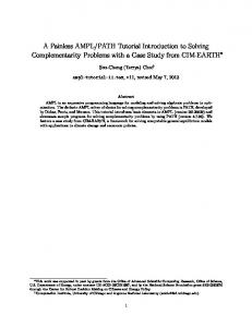
The electronic absorption spectrum of octahedral CrCl63- recorded in Cr3+ doped Cs2NaScCl6 (Figure 7 ) displays all three spin allowed d-d transitions, and in addition, the transitions from the 4A2 ground state into the 2Eg, 2T1g and 2T2g all due to spin flip transitions within the t2g3 ground state configuration.

Figure 7. 15 K absorption spectrum of 4.1% Cr(III): Cs2NaScCl6.



The design of the calculation follows similar considerations as in the hexamine complex studied in the previous section. However, the chlorine ligand has -orbitals available for bonding and also forms a more covalent ligand bond. Hence, we include the -type ligand orbitals. Due to the larger active space, the calculation is computationally more demanding than the amine system studied earlier. It is a good example to discuss a few option designed for larger active spaces. The complex has a large negative charge and thus a gas-phase calculation is certainly not the best choice. A good computational protocol should take into account the

19 environment effect for example by considering an ECP embedding together with point charges and much larger basis set. 15 For now we proceed with the gas-phase calculation. Following the protocol described in Section 2, the molecule is carefully placed into the xyz axis frame. The geometry is stored as “crcl6-03.xyz”. The CAS(3,5) calculation stateaveraged over 10 quartet roots and 9 doublet roots converges smoothly with the PAtom guess. ! SV def2/JK RI-JK conv PAtom xyzfile %MaxCore 1000 %casscf nel 3 norb 5 mult 4,2 nroots 10,9 end *xyz -3 4 Cr 0.000000 0.000000 0.000000 Cl 2.467400 0.000000 0.000000 Cl 0.000000 2.467400 0.000000 Cl 0.000000 0.000000 -2.467400 Cl 0.000000 -2.467400 -0.000000 Cl -2.467400 0.000000 0.000000 Cl 0.000000 -0.000000 2.467400 *

Thereafter, we visually inspect the doubly occupied space and identify the and bonding ligand orbitals depicted in Figure 8.



Figure 8. Ligand orbitals selected from the converged CAS(3,5) calculation. In our output these are the orbitals 46, 47, 51, 52 and 53.

For the CASSCF orbitals, there is a little mixing between -ligand orbitals and the 3dmetal orbitals. Their inclusion in the active space most probably does not affect the d-d spectrum. Nevertheless, we include the full set of ligand orbitals and run the CAS(13,10) calculation. The keyword “extorb doubleshell” is set in preparation of the next step that is the inclusion of the second d-shell. ! SV def2/JK RI-JK conv moread %moinp “cas_5.gbw” # converged CAS(3,5) orbitals

15 D. Maganas, M. Roemelt, M. Hävecker, A. Trunschke, A. Knop-Gericke, R. Schlögl, and F. Neese, Phys. Chem. Chem. Phys. 15, 7260 (2013).

20 %MaxCore 1000 # rotated ligand orbitals to be included in the active space 58-67 %scf rotate {47,61,90}{46,62,90}{53,58,90}{52,59,90}{51,60,90} end end %casscf nel 13 norb 10 mult 4,2 nroots 10,9 extorbs doubleshell # produces the second d-shell cistep accci # faster for multi-root calculations end *xyzfile -3 4 crcl6-03.xyz

We further extend the active space by the second d-shell orbitals. For the input above, these are the next five virtual orbitals. Inclusion of the entire second d-shell leads to a CAS(13,15), which is on the verge of the doable, but is a demanding calculation. To reduce the computational complexity, one could restrict the double-shell effect on the stronger occupied 3d-metal orbitals (t2g according to natural orbitals). In this case, the smaller CAS(13,13) needs to be considered. For CASSCF calculations with larger active spaces, ORCA features two spin-adapted alternatives to conventional full CI solvers · Density Matrix Renormalization Group approach (DMRG) developed in the Chan group.16 · Iterative Configuration Expansion (ICE), which is a variant of the CIPSI method proposed by Malrieu and coworkers. Both approaches are approximate solutions to the full-CI problem. Hence, less tight CASSCF convergence thresholds are sufficient and in fact recommended (etol 1e6). The setup of DMRG typically requires a bit more insight. There are excellent reviews on the subject.17,18 Here, we focus on the ICE approach. Note that the accuracy of ICE and DMRG can be systematically controlled – see the manual for more details. We calibrate the accuracy of the ICE methodology using the default settings for the CAS(13,13) before applying it to the larger CAS(13,15). ! SV def2/JK RI-JK conv ! moread %maxcore 4000 %moinp "cas_10.gbw" # converged cas(13,10) calculation with the # double shell ranging from 68-72 (t2g orbitals first) %casscf nel 13 norb 13 #or 15 if the full second d-shell is included mult 4,2 nroots 10,9 etol 1e-6 # default = 1e-7 cistep ice # approximate CI step for large active spaces end *xyzfile -3 4 crcl6_03.xyz

The results are summarized Table 3 together with the experimental values.19 The ICE(13,13) and the exact CAS(13,13) are practically identical. The extended ICE(13,15) improves the results in particular for quartet excitations. Already at this level of theory, the quartet transitions are in good agreement. The doublet excitations (low-spin) 16 Sharma, S.; Chan, G. K.-L. (2012) J. Chem. Phys., 136, 124121 17 T. Yanai, Y. Kurashige, W. Mizukami, J. Chalupský, T.N. Lan, and M. Saitow, Int. J. Quantum Chem. 115, 283 (2015).

18 R. Olivares-Amaya, W. Hu, N. Nakatani, S. Sharma, J. Yang, and G.K.-L. Chan, J. Chem. Phys . 142, 34102

(2015). 19 O.S. Wenger, H.U. Güdel, J. Chem. Phys. 114, 5832-5841, 2001

21 should be further corrected with inclusion of more dynamic electron correlation. To compare with experimental results, we should enlarge the basis and treat environment effects. Table 3. d-d transition energies for the [CrCL6]3- model complex. All calculations are done in the SV basis.

Excitations 4T 2 2E 2T 1 4T (1) 1 2T 2 2A 1 4T (2) 1

Exp. 11900 13545 14180 18500 20250 - 28500

CAS(13,13) ICE(13,13) 13954 13954 19100 19099 19700 19698 20110 20104 25923 25922 29964 29963 31352 31348

ICE(13,15) 12477 19059 19659 18442 25452 28354 28520

5 A comment on using ANO basis sets

Many practitioners of CASSCF are used to employ ANO basis sets. In fact, ANOs have a lot to recommend themselves. They are accurate and systematically extendable and they form an excellent basis for correlated calculations. The drawback of ANOs is the intrinsically high computational cost due to the large number of primitives in which the orbitals are expanded. While ORCA is certainly not fully optimized for ANO calculations, there is an integral program (orca_anoint) that makes use of the general contraction scheme that underlies ANO construction. There are a few tricks to help those calculations. First let us recall the ANO basis sets that are built into ORCA: # The ORCA ANO basis sets # # # # # # ! # ! # ! #

These are our own ANO basis sets described in Neese, F.; Valeev, E. F. Revisiting the Atomic Natural Orbital Approach for Basis Sets: Robust Systematic Basis Sets for Explicitly Correlated and Conventional Correlated ab initio Methods. J. Chem. Theory Comput. 2011, 7, 33-43. n= D, T, Q, 5, 6 ano-pVnZ similar, slightly extended ANO sets aug-pVnZ augmented with one more shell except for the highlest L-quantum number saug-pVnZ augmented with more s-functions

# # ! ! !

Other useful built-in ANO basis sets. A complete list is reported in the manual section 9.3.1 ANO-RCC-DZP ANO-RCC-TZP ANO-RCC-FULL

If the desired ANO basis is not available in ORCA, you can read or define the basis in the %basis block. Reading a basis from the EMSL is straight forward. Just select the elements and the “GAMESS US” format. Then copy and paste the basis set information in a text-file. In that case, it is very important to set the flag “ANOBasis true”! # Reading your own ANO basis set e.g. from the EMSL %basis GTOName “MyANOFile.bas” # for the format check the manual! # it is essentially EMSL Gamess US format ANOBasis true # this tells the program that it deals with ANOs

22 # !! IMPORTANT – YOU CAN NOT MIX ANO AND NON-ANO BASES!!

Now, let us revisit the [CrCL6]3- example from Section 4 with ANO basis sets. We use the resolution of the identity approximation and conventional integral storage in order to speed up the calculation. For small basis sets this should pretty much always be possible, even if the molecules are big. The PAtom guess is not available for ANO basis sets. Hence, we start with the default guess, inspect the orbitals and rotate accordingly (guess.gbw file). # ANO calculation # # ANO-RCC-DZP : double zeta ANO-RCC basis (should be used with DKH) # RI-JK : Use fitting for all integrals (critical for performance) # Conv : Store integrals on disk (critical for performance) !ANO-RCC-DZP DKH AutoAux ri-jk conv moread %moinp “guess.gbw” # rotated PModel guess with 3d orbitals active %casscf nel 3 norb 5 nroots 10 end * int -3 4 Cr 0 0 0 0.0000 0.000 0.000 Cl 1 0 0 2.4674 0.000 0.000 Cl 1 2 0 2.4674 90.000 0.000 Cl 1 2 3 2.4674 90.000 90.000 Cl 1 2 3 2.4674 90.000 180.000 Cl 1 2 3 2.4674 180.000 0.000 Cl 1 2 3 2.4674 90.000 270.000 *

There are no pre-defined auxiliary basis set for ANO-RCC. Thus we use the AutoAux construction, which generates a big decontracted auxiliary basis set that can be used in CASSCF / NEVPT2 calculations.20 From there on, everything is pretty much the same as in Section 4. However, at the DZP level, including the ligand orbitals we observe a trailing convergence as can be seen from the gradient progression below. ||g|| = 0.103578893 Max(G)= ||g|| = 0.027803852 Max(G)= ||g|| = 0.010459608 Max(G)= ... 20 iterations more ... ||g|| = 0.044716665 Max(G)= ||g|| = 0.022609157 Max(G)= ||g|| = 0.019453693 Max(G)= ||g|| = 0.028508328 Max(G)= ||g|| = 0.014822140 Max(G)= ||g|| = 0.018136280 Max(G)= ||g|| = 0.020715980 Max(G)= ||g|| = 0.020835649 Max(G)= ||g|| = 0.025479718 Max(G)=

0.031317337 Rot=134,38 0.005852422 Rot=132,8 0.002120086 Rot=141,38 -0.026700552 -0.015214902 -0.011320410 0.019778929 -0.006988486 -0.009782139 -0.013196297 0.011545400 -0.016634195

Rot=65,35 Rot=65,35 Rot=65,35 Rot=65,35 Rot=61,35 Rot=63,35 Rot=63,35 Rot=65,35 Rot=65,35

The program struggles with rotation 65-35. At this point we could play with the MaxRot settings or switch convergence strategy. This will certainly require some trial and error. In this particular case unrestricting the stepsize (MaxRot 5) does the job. In our experience, the “orbstep SuperCI / switchstep DIIS” combination is pretty robust and should be tried first when facing convergence problems with the default settings. Indeed convergence is achieved in 12 iterations. The remainder of this calculation proceeds smooth. We report the final results with the ANO-RCC basis sets in Table 4. The excitations energies have converged, but the results are still not optimal for 20 G.L. Stoychev, A.A. Auer, and F. Neese, J. Chem. Theory Comput. 13, 554 (2017).

23 the doublet transition and the highest quartet state. The results should improve with dynamical correlation. Table 4.d-d transition energies for the [CrCl6]3- model complex in cm-1.

Excitations

ANO-RCC TZP ICE(13,15) 263 MOs 4T 11900 12477 12093 2 2E 13545 19059 18799 2T 14180 19659 19485 1 4T (1) 18500 18442 18734 1 2T 20250 25452 25391 2 2A - 28354 27810 1 4T (2) 28500 28520 30504 1 a O.S. Wenger, H.U. Güdel, J. Chem. Phys. 114, 5832-5841, 2001

6

Exp.a

SV ICE(13,15) 99 MOs

ANO-RCC DZP ICE(13,15) 141 MOs 12466 18609 19275 19052 25216 27992 30942

ANO-RCC FULL ICE(13,15) 780 MOs 11992 18770 19467 18635 25354 27696 30369

[FeIV(O)(TMC)(MeCN)]2+ - covalent metal-ligand interactions and the computation of MCD / Mössbauer

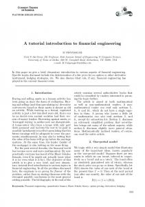
So far we have computed two Cr(III) model complexes, where the selection of the active space was straight forward and the ligand orbitals could be identified easily. However, this is not always the case. In the following example, we discuss strategies for systems where both the metal and ligand orbitals are more delocalized. Further we illustrate how to obtain the MCD spectra and Mössbauer parameters. We chose a classic oxo-iron(IV) complex as an example, [FeIV(O)(TMC)(MeCN)]2+ (TMC = 1,4,8,11-tetramethyl-1,4,8,11-tetraaza-cyclotetradecane), which has been spectroscopically characterized to feature a triplet (S=1) ground state with a low-lying quintet (S=2) state. Our major concern here is to compute reliable d-d transition energies. Specifically, we demonstrate that the CAS(4,5) calculation, i.e. including only the five metal d-orbitals and associated electrons, fails to predict accurate d-d transition energies. To improve the description, one has to enlarge the active space by incorporating ligand-based orbitals that strongly interact with the Fe d-orbitals. First, let us perform a CASSCF calculation involving the five metal d-orbitals only (Figure 9). The calculations are fairly large and should be executed on a cluster. For the same reason, we use the RI approximation to speed-up the calculations.

24



Figure 9. CASSCF(4,5) natural orbitals of the [FeIV(O)(TMC)(MeCN)]2+ complex.

We start with a structure that was optimized at the B3LYP level and is further denoted as “3_FeIV_FeO_TMC_B3LYP.xyz”. The origin is placed on the iron center. The molecule is aligned so that the O2- ligand points in z direction, x- and y-axis point to nitrogen ligands of the macrocyclic ring. # xyz coordinated corresponding to 3_FeIV_FeO_TMC_B3LYP.xyz * xyz 2 3 Fe 0.002998 -0.007344 0.001515 O -0.001116 -0.000277 1.630175 N 2.095349 -0.004573 0.097607 N 0.200201 2.113135 -0.058476 N -2.125671 0.063743 -0.055342 N -0.262696 -2.083062 0.099258 N 0.026185 -0.040306 -2.037309 C 2.379856 1.274701 0.818064 H 3.461553 1.463693 0.822094 H 2.049737 1.148041 1.850453 C 1.658766 2.417051 0.153944 H 2.100939 2.625540 -0.822455 H 1.760378 3.331135 0.750396 C -0.596737 2.654593 1.093961 H -0.443295 3.742414 1.111828 H -0.170268 2.236737 2.007879 C -2.096782 2.377084 1.031942 H -2.530900 2.871230 1.910687 H -2.547214 2.886931 0.172889 C -2.560266 0.924003 1.096929 H -2.195902 0.450687 2.010641 H -3.658578 0.907687 1.118175 C -2.609979 -1.345025 0.159227 H -3.529677 -1.331319 0.755585 H -2.872130 -1.758179 -0.816866 C -1.565990 -2.202307 0.823511 H -1.889548 -3.251614 0.831694 H -1.395726 -1.887484 1.854313 C 0.766571 -2.782101 0.930227 H 0.553252 -3.857800 0.873763 H 0.614242 -2.465696 1.965300 C 2.205440 -2.505017 0.533023 H 2.388950 -2.712817 -0.527779 H 2.833076 -3.216745 1.083469 C 2.659448 -1.112064 0.930432 H 2.362521 -0.920766 1.964913 H 3.753447 -1.034356 0.876226 C 2.786221 -0.008352 -1.220068 H 3.867100 0.090132 -1.060877 H 2.444812 0.817981 -1.841283 H 2.587643 -0.943763 -1.744176 C -0.183566 2.845719 -1.297287 H 0.021608 3.914507 -1.157466 H -1.238959 2.729346 -1.523970 H 0.403174 2.484394 -2.141228

25 C H H H C H H H C C H H H



-2.804306 -3.890506 -2.524644 -2.550379 -0.349394 -0.583090 0.602407 -1.127677 0.023227 0.016192 -1.003427 0.364485 0.679608

0.535065 0.472572 -0.097810 1.564826 -2.770800 -3.830433 -2.693001 -2.329378 -0.048464 -0.058200 0.121007 -1.032499 0.729029

-1.294551 -1.152725 -2.136085 -1.526693 -1.217076 -1.055842 -1.743597 -1.837385 -3.186690 -4.631548 -4.993410 -4.993982 -5.008050

*

Since we opt for the CAS(4,5) in the first run, we immediately start with PAtom as guess. In order to calculate the d-d transition energies, the CAS(4,5) calculation is averaged over ten triplet states using Def2-TZVP basis set. Once the calculation converges, we perform a NEVPT2 correction on top the CASSCF wave function to see how dynamic electron correlation affects the excitation energies. In the following input, we take a shortcut and immediately start with the triple zeta basis and the PAtom guess. PAtom automatically invokes a basis set projection from a singlet-zeta basis set. Hence, the initial gradient will be large. In addition, we expect more covalent bonds in this example (Figure 9), while PAtom produces very metal dominant orbitals. To avoid convergence problems, we switch to a less aggressive scheme that is “orbstep SuperCI” and “switchstep DIIS”. Note that the combination is particularly well suited to protect the active space using level shifts.21 # d-d excitations with the CAS(4,5) # def2-TZVP/C auxiliary basis (smaller compared to def2/JK) !Def2-TZVP def2-TZVP/C TightSCF RI-NEVPT2 PAtom PAL8 %maxcore 4000 %casscf nel 4 # d-electrons norb 5 # 3d-orbitals mult 3 # triplet states nroots 10 # calculate ten triplet states trafostep ri # speed up integral trafo orbtep SuperCI switchstep DIIS etol 1e-7 # reset etol: tightscf produces more accurate # integrals and unnecessarily increases etol. end



* xyzfile 2 3 3_FeIV_FeO_TMC_B3LYP.xyz

The CASSCF(4,5) calculation converges with the following composition of the wave function for each state and the transition energies relative to the ground-state. --------------------------------------------CAS-SCF STATES FOR BLOCK 1 MULT= 3 NROOTS=10 --------------------------------------------ROOT

ROOT

0: E= 0.95940 0.01268 0.01100 0.00832 0.00658 1: E= 0.72190 0.15436 0.06177 0.03150

[ [ [ [ [ [ [ [ [

-2235.4566946603 Eh 0]: 21100 3]: 20110 27]: 01120 7]: 12010 15]: 10210 -2235.4145918856 Eh 6]: 12100 1]: 21010 17]: 10120 10]: 11110

1.146 eV

21 unless the occupation number is exactly 2.0 or 0.0

9240.5 cm**-1

26 ROOT

ROOT

ROOT

ROOT

ROOT

0.02675 0.00250 2: E= 0.72571 0.15270 0.06835 0.03276 0.01150 0.00278 3: E= 0.96804 0.02283 0.00382 4: E= 0.35487 0.35479 0.16455 0.08673 0.01405 0.01298 0.00406 0.00298 0.00293 5: E= 0.27092 0.25558 0.23175 0.12533 0.08105 0.01255 0.00855 0.00514 6: E= 0.66060 0.22014 0.06492 0.03331 0.00857 0.00555 0.00378

[ [ [ [ [ [ [ [ [ [ [ [ [ [ [ [ [ [ [ [ [ [ [ [ [ [ [ [ [ [ [ [ [ [ [

25]: 01210 13]: 11011 -2235.4122540846 9]: 11200 3]: 20110 12]: 11020 22]: 02110 15]: 10210 0]: 21100 -2235.4035730634 10]: 11110 1]: 21010 25]: 01210 -2235.3816933395 10]: 11110 1]: 21010 6]: 12100 25]: 01210 4]: 20101 17]: 10120 13]: 11011 16]: 10201 8]: 12001 -2235.3809740494 7]: 12010 3]: 20110 15]: 10210 9]: 11200 22]: 02110 2]: 21001 12]: 11020 11]: 11101 -2235.3776909500 10]: 11110 1]: 21010 25]: 01210 6]: 12100 4]: 20101 16]: 10201 8]: 12001

Eh

1.209 eV

9753.6 cm**-1

Eh

1.446 eV

11658.8 cm**-1

Eh

2.041 eV

16460.9 cm**-1

Eh

2.060 eV

16618.8 cm**-1

Eh

2.150 eV

17339.3 cm**-1

Let us have a close look at the definition of the wave function predicted by CAS(4,5) calculation. The ground state wave function (ROOT 0) is dominated by the configuration 21100 (96%), corresponding to an electron configuration of (dxy)2(dxz)1(dyz)1(dx20 0 y2) (dz2) . The first two excited states; ROOT 1 and ROOT 2 appear close to each other with excitation energies 9240.5 and 9753.6 cm–1, respectively. These two excited states are dominated by electronic configurations 12100 and 11200, representing the transitions of dxy ® dxz and dxy ® dyz, respectively. Roots 3 and 6 are the dxy ® dx2-y2 transition. This is a shell-opening excitation, in which the number of the unpaired electron increases from two to four. As a consequence, this single excitation gives rise to five excited states in total. For more detailed discussion, we refer to the article of Ye et al.22 The following higher energy excited states are mainly the excitations from dxz/yz to the dx2-y2 (roots 4 and 5) and dz2 orbitals. The remaining transitions are mainly twoelectron excitations. The successive NEVPT2 calculation on top of the CAS(4,5) wave function gives the following excitation energies. In comparison with the experiment,23 the computed excitation energies are significantly overestimated (Table 5). ----------------------------NEVPT2 TRANSITION ENERGIES

22 Ye, S.; Xue, G.; Krivokapic, I.; Petrenko, T.; Bill, E.; Que, L., Jr; Neese, F., Chem. Sci. 2015, 6, 2909–2921 23 Decker, A.; Rohde, J.-U.; Klinker, E. J.; Wong, S. D.; Que, L.; Solomon, E. I. J. Am. Chem. Soc. 2007, 129, 15983–15996.

27 -----------------------------LOWEST ROOT (ROOT 0, MULT 3) =



STATE ROOT MULT 1: 1 3 2: 2 3 3: 3 3 4: 4 3 5: 5 3 6: 7 3 7: 6 3 8: 8 3 9: 9 3

DE/a.u. 0.063387 0.065484 0.093119 0.095106 0.099514 0.101362 0.103407 0.112200 0.159447

-2240.056906237 Eh -60955.047 eV

DE/eV 1.725 1.782 2.534 2.588 2.708 2.758 2.814 3.053 4.339

DE/cm**-1 13911.8 14372.1 20437.2 20873.4 21840.8 22246.3 22695.2 24625.0 34994.7

Now we run a CASSCF calculation incorporating the ligand-based orbitals. In order to design a balanced active-space that can deliver correct reference wave function, we need to understand the bonding of the complex. The TMC ligand is a tetradentate ligand, which form metal-ligand σ bond through the four equatorial N donors (σ-Neq). The oxoligand forms very strong covalent bonds with the iron center involving one σ (σ-O) and two π (2 x π-O) bonds. The axial MeCN also forms a σ bond (σ-Nax) with iron. Both σ-O and σ-Nax simultaneously interact with Fe-3dz2 with a single bonding orbital that needs to be included in the active space. Hence, the active space should contain four bonding and the corresponding anti-bonding orbitals, in addition to the non-bonding Fe-3d xy orbital. The complete active space is therefore constructed by twelve-electron distributing over nine orbitals, CAS(12,9).

Figure 10. CASSCF(12,9) natural orbitals of the [FeIV(O)(TMC)(MeCN)]2+ complex.

For the model complexes studied earlier, we could easily identify the ligand orbitals,

28 extend the active space and re-converge the calculation. Inspecting the doubly occupied orbitals (range 0-96) in the converged CAS(4,5) calculation, we are not able to properly select all four ligand orbitals depicted in Figure 10. The -ligand orbitals are entirely missing. The majority of ligand orbitals do not have significant weight on the metal-d orbitals e.g. Figure 11 illustrates how delocalized the canonical dx2-y2-ligand orbital is. Such orbitals would make a poor guess for the CASSCF(12,9) calculation and most probably lead to convergence problems.

Figure 11. CAS(4,5) dx2-y2 ligand orbitals



--------------------------------------------CAS-SCF STATES FOR BLOCK 1 MULT= 3 NROOTS=10 ---------------------------------------------

From here, it is difficult to improve the CAS(4,5) orbitals. In our experience, for covalent systems, QROs from DFT work well. Thus we proceed with QROs using the BP functional.



# def2/J RI auxiliary basis for pure DFT functionals !BP def2-TZVP def2/J UNO pal8 %maxcore 4000 *xyzfile 2 3 3_FeIV_FeO_TMC_B3LYP_rotate-1.xyz

Figure 12 shows the ligand guess orbitals that we have selected. The QROs are not “pure”, but at least the -ligand orbitals are present from the start.

29

Figure 12. Ligand orbitals selected QROs generated with the BP functional.

The CAS(12,9) output shows the familiar composition for the ground state and excited state wave functions. --------------------------------------------CAS-SCF STATES FOR BLOCK 1 MULT= 3 NROOTS=10 --------------------------------------------ROOT

0: E= 0.81233 0.04129 0.02851 0.02800 0.01427 0.00717 0.00598 0.00581 0.00432 0.00407 0.00406 0.00393 0.00294 0.00272

[ [ [ [ [ [ [ [ [ [ [ [ [ [

-2235.6380115533 Eh 1469]: 222221100 1297]: 221122200 1019]: 211222101 1089]: 212121201 874]: 202221102 1462]: 222212010 1454]: 222210210 1442]: 222201120 737]: 122221110 684]: 122121210 614]: 121222110 774]: 201122202 232]: 022221120 466]: 112221111

A closer look to the configurations generated by CASSCF(12,9) calculation reveals that the ground state (ROOT 0) is dominated by the configuration 222221100 (81%), which corresponds to (σx2-y2)2(σz2)2(πxz/yz)4(dxy)2(π*xz/yz)2(σ*x2-y2)0(σ*z2)0. Following the same route, one can assign the other excited states. The successive NEVPT2 calculation on top of a CASSCF(12,9) wave function gives ----------------------------NEVPT2 TRANSITION ENERGIES -----------------------------LOWEST ROOT (ROOT 0, MULT 3) = STATE ROOT MULT 1: 1 3 2: 2 3 3: 3 3 4: 4 3 5: 8 3 6: 9 3 7: 5 3

DE/a.u. 0.052356 0.053857 0.058998 0.059058 0.059486 0.061982 0.062996

-2240.054966242 Eh -60954.995 eV

DE/eV 1.425 1.466 1.605 1.607 1.619 1.687 1.714

DE/cm**-1 11490.8 11820.2 12948.6 12961.8 13055.6 13603.5 13826.1

30 8: 9:

6 7

3 3

0.073581 0.075884

2.002 2.065

16149.1 16654.5

Comparison of the major d-d transition energies at the CASSCF(4,5)/NEVPT2 and CASSCF(12,9)/NEVPT2 levels to the experimental values below. Table 5. NEVPT2 Excitation energies for the [FeIV(O)(TMC)(MeCN)]2+ complex

d-d transitions xz/yz → x2-y2 xy → xz/yz

NEVPT2 NEVPT2 Exp. CAS(4,5) CAS(12,9) 20873, 21840 11490, 11820 ~10600 13911, 14372 13055, 13603 ~12900

Clearly the CASSCF(4,5)/NEVPT2 calculation significantly overestimates the transition energies. While the transition energies predicted by CASSCF(12,9)/NEVPT2 agree reasonably well with the experiment. This shows the importance of a balanced active space and incorporation of the ligand orbitals. The observation simply reflects the fact that a proper description of a covalent bond requires both bonding and antibonding orbitals in the active space. This is a well-known protocol for studying bondbreaking and bond-formation. Furthermore, in this situation, balancing the active space improves the CASSCF convergence. A remark on the character of the CASSCF orbitals: For the current complex with covalent Fe–O bonds, the CASSCF(4,5) calculation predicts ionic anti-bonding π-orbitals (88% Fe), whereas the CASSCF(12,9) calculation accurately predicts covalent anti-bonding orbitals (62% Fe + 35% O). Judging the covalency based on the unbalanced CASSCF(4,5) orbitals is dangerous!

6.1 Calculation of MCD spectra and Quadrupole splitting Below is the input for a CASSCF/NEVPT2 calculation of the MCD spectrum. The underlying physics are beyond the scope of this tutorial. The methodology is described elsewhere. 24 Here, we briefly show how the MCD spectra can be computed with CASSCF. A careful analysis of the MCD results can be found in the article of Ye et al.25 The MCD intensity is dominated by the spin-allowed transition. Hence, the previously computed triplet d-d manifold should be sufficient. The computation involves transitions from all microstates (all MS values). The corresponding keyword is “NInitStates”. For the 10 non-relativistic triplet roots, there are 30 microstates (or ‘magnetic sublevels’ – these are the three MS sublevels for each of the ten triplet states). !Def2-TZVP Def2-TZVP/C TightSCF RI-NEVPT2 !MOREAD %moinp "3_FeIV_FeO_TMC_CAS_12-9_10T_c.gbw" %pal nprocs 8 end %maxcore 4000 %casscf nel 12 norb 9 mult 3 nroots 10

24 Ganyushin, D.; Neese, F., J. Chem. Phys. 2008, 128, 114117

25 Ye, S.; Xue, G.; Krivokapic, I.; Petrenko, T.; Bill, E.; Que, L., Jr; Neese, F., Chem. Sci. 2015, 6, 2909–2921

31 TrafoStep ri rel dosoc true mcd true NInitStates 30

# # # # #

enter into relativistic calculation perform spin-orbit coupling perform the MCD calculation number of SOC state to account starts from the lowest state NPointsTheta 10 # number of integration points for NPointsPhi 10 # Euler angles NPointsPsi 10 B 70000, 70000, 70000, 70000, 70000, 70000 # experimental # magnetic field # strength in Gauss Temperature 2, 10, 20, 40, 60, 80 # experimental # temperature (in K) end end *xyzfile 2 3 3_FeIV_FeO_TMC_B3LYP.xyz

In the input file, the parameters magnetic field (B) and temperature are assigned in pairs, i.e. B = 70000, 70000, 70000, . . . Temperature = 2, 10, 20. . . . The program calculates MCD and absorption spectra for every pair. ORCA calculates the strength of left circular polarized (LCP) and right circular polarized (RCP) transitions and prints the transition energies, the difference between LCP and RCP transitions (intensity denoted as C), and sum of LCP and RCP transitions (absorption intensity denoted as D), and C by D ratio for every pairs of B and temperatures. ----------------------------------------------------------MCD Transitions B = 70000.00 Gauss T = 2.000 K ----------------------------------------------------------C D C/D ----------------------------------------------------------0 -> 1 -0.00000 0.00154 -0.00004 0 -> 2 0.00000 0.00114 0.00005 0 -> 3 -0.00000 0.00000 -0.01153 0 -> 4 0.00000 0.00001 0.00050 0 -> 5 -0.00004 0.51146 -0.00008 0 -> 6 0.00004 0.33632 0.00012 0 -> 7 0.00000 0.03891 0.00000 0 -> 8 -0.00000 1.80573 -0.00000 0 -> 9 0.00000 0.39352 0.00001 0 -> 10 0.00000 32.45677 0.00000 0 -> 11 -0.00000 26.68497 -0.00000 0 -> 12 0.00001 0.87862 0.00001 0 -> 13 -0.00001 4.05381 -0.00000 0 -> 14 0.00000 0.01267 0.00001 0 -> 15 -0.00000 0.12560 -0.00000 0 -> 16 0.00000 1.51414 0.00000 0 -> 17 -0.00000 1.05308 -0.00000 0 -> 18 0.00001 0.94487 0.00001 0 -> 19 -0.00001 1.22514 -0.00000 0 -> 20 -0.00001 0.09362 -0.00008 0 -> 21 0.00001 0.09371 0.00008 0 -> 22 0.00000 0.05183 0.00000 0 -> 23 0.00000 1.06355 0.00000 0 -> 24 -0.00000 0.00739 -0.00001 0 -> 25 0.00000 0.00178 0.00004 0 -> 26 0.00000 0.06958 0.00000 0 -> 27 -0.00000 0.66457 -0.00000 0 -> 28 0.00000 0.16718 0.00000 0 -> 29 0.00000 0.91598 0.00000 0 -> 30 -0.00000 0.03829 -0.00001 0 -> 31 0.00000 0.72897 0.00000 0 -> 32 0.00000 0.33647 0.00000 0 -> 33 -0.00000 0.48522 -0.00000 0 -> 34 0.00000 0.42774 0.00000 1 -> 2 0.00000 0.00000 0.00005 1 -> 3 -0.00000 0.00002 -0.02590 1 -> 4 0.00000 0.00002 0.01821 1 -> 5 0.00000 0.00012 0.00000

32 In addition to the output, a successful calculation generates a series of files named like input.1.casscf.mcd. The numbering identifies the magnetic field/ temperature pair specified in the input. Since, we specified six pairs in the input, there should be files numbered from 1 to 6. In case of NEVPT2, the files are named input.1.nevpt2.mcd respectively. One can use orca-mapspc program to plot the predicted MCD spectra. For details about orca_mapspc, please consult the orca manual. The keywords x0 and x1 define the energy of the plot. orca_mapspc input.1.nevpt2.mcd MCD -x04000 -x120000 -w2000

Here the interval for the spectra generation is set from 4000 cm–1 to 20000 cm–1, and the line shape parameter is set to 2000 cm–1. If everything worked out fine, the program prints a summary and produces a “.dat” file with the same name prefix. Mode is MCD Cannot read the *.mcd.inp file ... taking the line width parameter from the command line Number of peaks

... 66917

Start wavenumber [cm-1]

...

4000.0

Stop wavenumber [cm-1]

...

20000.0

Peak FWHM [cm-1]

...

Number of points

... 1024

2000.0

The dat file has 7 columns entries, where the first column is the energy. The next three columns are the Gaussian convolution data points for the C , D and the ratio C/D. The last three columns the discrete peaks (C,D and C/D). For a temperature of 2K, the resulting MCD spectrum is depicted in Figure 13. The complete temperature depending MCD spectra can be found in the article Ye et al.26

26 Ye, S.; Xue, G.; Krivokapic, I.; Petrenko, T.; Bill, E.; Que, L., Jr; Neese, F., Chem. Sci. 2015, 6, 2909–2921.

33

Figure 13. MCD spectra for a temperature of 2K.

6.2 Mössbauer Parameters



The example input below shows how to calculate the Mössbauer parameters for the iron complex using the CASSCF wave function. The orca_eprnmr module typically applies to single reference methods. The Mössbauer parameters are an exception in this program. Here we directly use the previously converged CAS(12,9) wave function and add the necessary keywords to the %eprnmr block. Note that the %eprnmr block must be placed below the coordinate block. As a reminder, the quadrupole splitting is a ground state property. It is thus important to restrict the calculation to nroots=1 to get the ground-state density. Do not use the state-averaged density for the computation of Mössbauer Parameters! NEVPT2 is omitted, since the NEVPT2 density is not yet available (it is important to understand that the NEVPT2 procedure only corrects the energy, not the wave function and hence also not the density!). !Def2-TZVP Def2-TZVP/C TightSCF !MOREAD %moinp "CAS_9_10Roots.gbw" # converged CAS(12,9) with 10 triplet roots. %pal nprocs 8 end %maxcore 4000 %casscf nel 12 norb 9 mult 3 nroots 1 TrafoStep ri end *xyzfile 2 3 3_FeIV_FeO_TMC_B3LYP.xyz



%eprnmr Nuclei = all Fe {fgrad, rho} end

34 The output file should contain the following lines at its end, where you obtain the calculated quadrupole splitting (Delta-EQ) directly and the RHO(0)value (the electron density at the iron nucleus). ----------------------------------------ELECTRIC AND MAGNETIC HYPERFINE STRUCTURE --------------------------------------------------------------------------------------------------Nucleus 0Fe: A:ISTP= 57 I= 0.5 P= 17.2798 MHz/au**3 Q:ISTP= 57 I= 0.5 Q= 0.1600 barn ----------------------------------------------------------Tensor is right-handed. Raw EFG matrix (all values in a.u.**-3): -0.1898 0.0177 -0.1423 0.0177 -0.1922 0.1536 -0.1423 0.1536 0.3820 V(El) V(Nuc)

-0.2058 0.0325 ---------V(Tot) -0.1733 Orientation: X 0.7327196 Y 0.6805305 Z -0.0005219

-0.1844 -0.0909 ----------0.2754

0.3902 0.0585 ---------0.4487

0.6485519 -0.6980558 0.3034774

0.2061613 -0.2227023 -0.9528385

Moessbauer quadrupole splitting parameter (proper coordinate system) e**2qQ = 16.890 MHz = 1.456 mm/s eta = 0.228 Delta-EQ=(1/2{e**2qQ}*sqrt(1+1/3*eta**2) = 8.517 MHz = 0.734 mm/s RHO(0)= 11586.879407946 a.u.**-3

The calculated quadrupole splitting (0.734 mm/s) agrees very well with the experiment value of 1.24mm/s,27 which again credence our chosen active space.

7 [Co(SH)4]2- - Optical and Magnetic properties 7.1 Electronic Structure In ideal Td geometry, the tetracoordinate Co(II) complexes possess a 4A2 ground state, with a half-filled t2 subshell. The important single excitations within the metal d-shell are those from the doubly occupied e-orbitals (dz2 and dx2−y2) to the singly occupied t2set (dxy, dxz, and dyz). These excitations give rise to two quartet-excited states (4T1 and 4T ). Under conditions favoring further symmetry lowering, there will be further 2 splitting of the x, y, z components of the T states, such that T2x≡1-Ex, T2y≡1-Ey, T2z≡Bz and T1x≡2-Ex, T1y≡2-Ey, T1z≡Az in ~ S4 symmetry.

27 Rohde, J.-U.; In, J.-H.; Lim, M. H.; Brennessel, W. W.; Bukowski, M. R.; Stubna, A.; Münck, E.; Nam, W.; Que, L. Jr. Science 2003, 299, 1037–1039.

35



Figure 14. The metal d-based MOs of the model complex [Co(SH)4] 2-. Final state term symbols arising from single excitations are analyzed under approximate S 4 symmetry. The indicated orbital occupation pattern refers to the 4A2 ground state.

7.2 Setting up the CASSCF/NEVPT2 calculation

A general input for performing optical and magnetic properties calculations within the CASSCF/NEVPT2 methodology for the pseudo tetrahedral Co II (S=3/2) model complex (Figure 14) is provided below: ! def2-TZVP def2-TZVP/C PAtom PAL4 %casscf nel 7 norb 5 #7 electrons in 5 d orbitals nroots 10,35 mult 4,2 # 10 quartet and 35 doublet states trafostep RI #-----------------------------------------------nevpt2 SC #Perform the SC-NEVPT2 correction #-----------------------------------------------rel #flag for relativistic properties printlevel 3 #Control the amount of printing dosoc true #Do the SOC calculation #----------------------------------------------mcd true # Request the MCD calculation NInitStates 28 # Number of Donor SOC states # for the ABS and MCD spectra evaluation NPointsTheta 10 # Number of integration point for NPointsPhi 10 # Euler angles NPointsPsi 10 # B 5000 # Experimental Magnetic field (in Gauss) Temperature 10 # Experimental temperature (in K) #----------------------------------------------gtensor true # Request the G-tensor Calculation #----------------------------------------------dtensor true # Request the ZFS-tensor Calculation #(default if dosoc true) #----------------------------------------------end end * xyz -2 4 Co 0.000089000 S -1.194914000

0.000270000 1.441126000

0.000180000 -1.471908000

36 S S S H H H H *

-1.394869000 1.120414000 1.467145000 2.291750000 -1.704914000 -2.260149000 1.675644000

-1.170677000 -1.419512000 1.145600000 1.687013000 2.280708000 -1.693145000 -2.271185000

1.534517000 -1.549797000 1.486755000 0.542215000 -0.523177000 0.616185000 -0.637921000

In this protocol the minimal active space (3d orbitals) is chosen to be a CAS(7,5). As seen in the Section 5, CASSCF orbitals restricted to the 3d-metal orbitals are very ionic. In this example the converged CASSCF orbitals have more than 89% metal character according to the Loewdin population analysis. Thus, the PAtom guess is the ideal choice for such a setup. NEVPT2 is performed on top of the converged state averaged CASSSCF wave function. It should recover a major part of the dynamic electron correlation between the ground and the excited states. The calculation is carried out on the basis of all 10 roots for the quartet states (arising from the 4F and 4P terms of Co2+) together with 35 doublet roots (arising from the 2G, 2H, 2F, 2P, 2D terms of Co2+). Furthermore, in order to avoid unrealistic description of the ground state due to the state averaging the energetically higher second 2D term (accounting for the rest 5 doublet roots) is excluded. The output contains the following CASSCF and NEVPT2 transition energies. ----------------------------SA-CASSCF TRANSITION ENERGIES -----------------------------LOWEST ROOT (ROOT 0 ,MULT 4) =

-2974.012986842 Eh -80927.008 eV

STATE ROOT MULT DE/a.u. DE/eV DE/cm**-1 1: 1 4 0.003979 0.108 873.3 2: 2 4 0.015774 0.429 3462.0 3: 3 4 0.015782 0.429 3463.7 4: 4 4 0.019875 0.541 4362.0 5: 5 4 0.019882 0.541 4363.5 6: 6 4 0.024591 0.669 5397.1 7: 0 2 0.088630 2.412 19452.0 8: 1 2 0.088764 2.415 19481.5 9: 2 2 0.089205 2.427 19578.2 10: 3 2 0.089210 2.428 19579.3 11: 4 2 0.089837 2.445 19716.9 12: 5 2 0.090128 2.453 19780.8 13: 6 2 0.093332 2.540 20483.9 ---------------------------------------------

----------------------------NEVPT2 TRANSITION ENERGIES -----------------------------LOWEST ROOT (ROOT 0, MULT 4) =

-2975.223602565 Eh -80959.950 eV

STATE ROOT MULT DE/a.u. DE/eV DE/cm**-1 1: 1 4 0.005873 0.160 1288.9 2: 2 4 0.023207 0.631 5093.3 3: 3 4 0.023218 0.632 5095.8 4: 4 4 0.029850 0.812 6551.3 5: 5 4 0.029857 0.812 6552.9 6: 6 4 0.035846 0.975 7867.4 7: 2 2 0.083339 2.268 18290.9 8: 3 2 0.083349 2.268 18293.0 9: 0 2 0.083708 2.278 18371.9 ---------------------------------------------

37 Inspection of the states composition shows that the first 6 quartet excited states correspond to the z and xy components of the 4T2 and 4T1 final states, respectively (Figure 14). --------------------------------------------CAS-SCF STATES FOR BLOCK 1 MULT= 4 NROOTS=10 --------------------------------------------ROOT ROOT ROOT

ROOT

ROOT

ROOT

ROOT ROOT ROOT

ROOT

0: E= 0.99920 1: E= 0.99920 2: E= 0.54004 0.37209 0.05208 0.03120 0.00362 3: E= 0.53816 0.37324 0.05251 0.03144 0.00373 4: E= 0.66405 0.20722 0.05145 0.04247 0.02355 0.01126 5: E= 0.66485 0.20578 0.05167 0.04300 0.02354 0.01115 6: E= 0.70304 0.29695 7: E= 0.70300 0.29693 8: E= 0.50849 0.23066 0.21146 0.04933 9: E= 0.50777 0.23074 0.21226 0.04913

[ [ [ [ [ [ [ [ [ [ [ [ [ [ [ [ [ [ [ [ [ [ [ [ [ [ [ [ [ [ [ [ [ [ [ [

-2974.0129868416 9]: 22111 -2974.0090077771 8]: 21211 -2973.9972125969 4]: 12121 7]: 21121 1]: 11212 3]: 12112 6]: 21112 -2973.9972050318 3]: 12112 6]: 21112 2]: 11221 4]: 12121 7]: 21121 -2973.9931121667 2]: 11221 3]: 12112 1]: 11212 6]: 21112 7]: 21121 4]: 12121 -2973.9931051642 1]: 11212 4]: 12121 2]: 11221 7]: 21121 6]: 21112 3]: 12112 -2973.9883958910 0]: 11122 5]: 12211 -2973.9179925415 5]: 12211 0]: 11122 -2973.9171526473 7]: 21121 1]: 11212 4]: 12121 6]: 21112 -2973.9171455718 6]: 21112 2]: 11221 3]: 12112 7]: 21121

Eh Eh

0.108 eV

873.3 cm**-1

Eh

0.429 eV

3462.0 cm**-1

Eh

0.429 eV

3463.7 cm**-1

Eh

0.541 eV

4362.0 cm**-1

Eh

0.541 eV

4363.5 cm**-1

Eh

0.669 eV

5397.1 cm**-1

Eh

2.585 eV

20848.8 cm**-1

Eh

2.608 eV

21033.2 cm**-1

Eh

2.608 eV

21034.7 cm**-1

7.3 Optical spectra Based on these excited states several spectra including Absorption, CD (Circular Dichroism) and SOC corrected Absorption spectra (provided that relativistic calculations have been requested) are generated. These spectra can be extracted by using the orca_mapspc utility. The orca_mapspc program applies Gaussian/Lorenzian type line shape functions to the calculated transitions with a user-defined “full width at half maximum” (FWHM) value. One has to provide some information for the program such as the name of the output file, the type of the desired spectrum and the energy range. # The lines below are shell commands that call orca_mapspc directly # myfile.out is the output of the previous calculation.

38 orca_mapspc myfile.out ABS –x05000 –x125000 –w1500 –n10000 orca_mapspc myfile.out SOCABS –x05000 –x125000 –w1500 –n10000 orca_mapspc myfile.out CD –x05000 –x125000 –w1500 –n10000

The output contains CASSCF and NEVPT2 results. The orca_mapspc program processes both results. In the following we focus on the NEVPT2 results. In Figure 15 (top) the respective Absorption and SOC corrected Absorption spectra for [Co(SH)4]2- are presented in the energy range 0 -10000 cm-1. As can be seen the Absorption spectrum is dominated by electron excitations into the 1 - 4 E x , y , 2 - 4 Ex, y and 4 Az (Figure 15, top left and Figure 1). Moreover, switching on the SOC effects a more complicated spectral pattern is observed owning to the nature of the contributing Ms states (Figure 15, top right). This can modify the intensity, the shape as well as the energy distribution of the spectrum. In general, this is expected to be more pronounced in higher energy areas, which are dominated, by states of different multiplicities (Figure 15, bottom left and right).









Figure 15. NEVPT2 Visible Absorption and SOC corrected Absorption spectra of [Co(SH)4]2-



39

7.4 G-tensor

CASSCF provides two methodologies that can deliver information about the g-tensors. These are: · The Effective Hamiltonian method.28 which provides information about the principal g values and it is hence valid for every spin case (Kramers or nonKramers systems) · The quasi-degenerate perturbation theory (QDPT) is valid for an individual Kramers doublet. In fact, for a system with odd electrons (non-integer spin cases or Kramers systems) the doubly degenerate eigenvalues obtained from the QDPT procedure represent Kramers pairs. Hence one can obtain information about the effective g values of an isolated Kramers doublet assuming pseudo spin S=½. Let us first inspect the g values estimated by the Effective Hamiltonian method. ---------------------------------------------ELECTRONIC G-MATRIX FROM EFFECTIVE HAMILTONIAN ---------------------------------------------g-matrix: 2.243559 -0.000120 0.018210

-0.000189 2.242967 -0.006289

g-factors: 2.242915

2.243117

2.996329 iso =

2.494120

g-shifts: 0.240596

0.240798

0.994009 iso =

0.491801

Eigenvectors: X 0.012637 Y 0.999888 Z 0.008029

0.999627 -0.012438 -0.024317

0.018262 -0.006258 2.995835

0.024214 -0.008333 0.999672

# The g-factors are square roots of the eigenvalues of gT*g # Orientations are the eigenvectors of gT*g

The output shows total g-matrix followed by the three principal components and their orientation, where the orientation (eigenvectors). Note that the eigenvectors are printed as column vectors – see color coding. The orientation can also be used to rotate the molecule into the eigenframe of the g-tensor – simply multiple the xyz coordinates with the orientation tensor. In this example, we obtain gz=2.99 and gx,y=2.24. Furthermore knowing the ratio of the g-values (gz/gx,y=1.3) and the orientation (eigenvectors) of the g tensor in the molecular axis frame one can be visualize the gtensor components (See Figure 16).

28 Atanasov, M.; Aravena, D.; Suturina, E.; Bill, E.; Maganas, D.; Neese, F.; Coord. Chem.. Rev. 2015, 289-290 (0), 177-214

40



Figure 16. Orientation of the g tensor components in the molecular frame

In general, the g-values are only influenced by spin-allowed (spin-conserving) transitions. Analysis from the individual states reveals the only states that contribute are those that can interact via spin-orbit coupling with the ground state. Hence only the first three states contribute. According to the expectations from the LFT,29 the g values are mainly dominated by single electron excitations into the T 2 states: 4A2→4Ex (dx2-y2→dxz), 4A →4Ey (d 4 4 z 4 z 2 x2-y2→dyz) and A2→ A2 (or B )(dx2-y2→dxy). The largest positive g-shift is calculated for the gz parameter, due to the strong SOC effect of the excited 4Bz on the 4A2 ground state. Additionally, the effective g'-tensors, arising from a particular Kramers doublet serves a diagnostic tool for the composition of the ground state Kramers doublet and thus possibly the sign of zero field splitting D. -------------KRAMERS PAIR 1 -------------g-factors: 0.003963

0.005248

8.870597 iso =

2.959936

4.384133

4.385082 iso =

4.047917

-------------KRAMERS PAIR 2 -------------- g-factors: 3.374535

As can be seen the ground state Kramers doublet represents an axial system with = g z' 8.9, g x' , y < 0.1 . On the other hand the second Kramers pair represents a rhombic system with = g z' 3.4 = g x' , y 4.4 . This indicates that the ground state Kramers doublet is composed of = M s ± 3 / 2 . In fact by inspecting the composition of the calculated SOC states this is exactly what is observed:

29 Neese, F.; Solomon, E. I., Magnetoscience - Molecules to Materials. Miller, J.S.;Drillon, M. ed.; 2003; Vol. IV, p 345

41 Eigenvectors: STATE

0:

0.0000

STATE

1:

0.0000

STATE

2:

130.5095

STATE

3:

130.5095



Weight

Real

Image

: Block Root

Spin

Ms

0.819191 0.169283

-0.099210 0.408961

0.899638 : 0.045101 :

0 0

0 1

3/2 3/2

0.819191 0.169283

0.876339 0.102883

-0.226321 : 0.398370 :

0 0

0 1

3/2 -3/2 3/2 -3/2

0.873822 0.029847 0.061898

-0.927664 -0.023661 -0.011361

-0.115162 : 0.171136 : -0.248534 :

0 0 0

0 1 0

3/2 1/2 3/2 1/2 3/2 -1/2

0.061898 0.873822 0.029847

-0.244423 -0.017317 -0.172762

-0.046429 : 0.934624 : -0.000803 :

0 0 0

0 0 1

3/2 1/2 3/2 -1/2 3/2 -1/2

3/2 3/2

7.5 D-tensor

If the calculation of the D-tensor is requested, (e.g. D tensor true), both the 2nd Order PT approach30 as well as the Effective Hamiltonian Method are used to evaluate the sign and the value of the zero field splitting D (note that if the SOC flag is on and the total spin of the system is S>1/2 this information is printed by default). In general both approaches are adequate in calculating the D-tensor18 (and references there in). In the case of [Co(SH)4]2- and in accordance with the discussion above both approaches predict an axial system with E/D~0 and negative D. However the 2nd order PT approach overestimates D by a factor of 1.5. As shown elsewhere18,31, in the presence of low lying excited states (< 1000 cm-1), which contribute through SOC with the ground state, the 2nd order PT methodology is not valid for the calculation zero-field splitting (ZFS). Under such circumstances, the D values must be analyzed carefully. -------------------------------------------ZERO-FIELD SPLITTING (2ND ORDER SPIN-ORBIT COUPLING CONTRIBUTION) --------------------------------------------



… Direction X=1 Y=2 Z=0 D = -101.374638 cm-1 E/D = 0.000096 -------------------------------------------------------ZERO-FIELD SPLITTING (EFFECTIVE HAMILTONIAN SPIN-ORBIT COUPLING CONTRIBUTION) -------------------------------------------------------Direction X=1 Y=2 Z=0 D = -65.254746 cm-1 E/D = 0.000096

Furthermore, analysis of the individual contributions to the D-tensor shows that once again the major contributions to the ZFS originates from 4T2 states dominated by 4A →4Ex (d 4 4 y 4 4 z 4 z 2 x2-y2→dxz), A2→ E (dx2-y2→dyz) and A2→ A2 (or B )(dx2-y2→dxy) single electron excitations. Moreover, significant contributions are observed from the respective 2T2 states. 30 Neese, F. and Solomon, E. I., Inorg. Chem. 1998, 37, 6568 31 Maganas, D.; Sottini, S.; Kyritsis, P.; Groenen, E. J. J.; Neese, F., Inorg. Chem. 2011, 50 (18), 8741-8754

42 Individual contributions to D-tensor: Block Mult Root D E 0 4 0 0.000 0.000 0 4 1 -103.443 -0.000 0 4 2 15.503 -15.344 0 4 3 15.489 15.328 … 1 2 6 6.678 -0.000 1 2 7 -2.391 1.707 1 2 8 -2.390 -1.707 …

8 Cu-dimer J-Couplings with NEVPT2, DLPNO-NEVPT2 and MRCI The Copper dimer [Cu(tmeen)(OH)]2Br2 shown in Figure 17 is a toy system, where a number of theoretical methods have been exercised. In this section, we study the singlettriplet splitting. The two Cu2+ atoms of the dimer have a [Ar]3d9 electronic configuration and therefore have one magnetic electrons each. This Cu dimer which we shall call Cu2(OH)2 henceforth, has an anti-ferromagnetic coupling constant of Jexp=-509cm-1 between the two magnetic centers.32 In the following, we use the crystal structure with optimized hydrogen positions (cu2.xyz). The minimal active space describing the singlet-triplet splitting is a CAS(2,2). The quality of ab initio results strongly depends on the methodology and it has been shown that such a minimal CAS does not work for multireference perturbation theory (e.g. NEVPT2).33

Figure 17: The two (localized) magnetic orbitals of Cu2(OH)2.

For the purpose of the tutorial, we use only small basis set (SV) and omit relativistic effects. Nevertheless, the example with ~500 basis function is rather big. It is a perfect opportunity to discuss the usage of the RI approximation in the context of multireference methods (Section 8.3). Note that Cu complexes are known to cause convergence problems due to the fully packed 3d shells. Therefore, we also discuss some common issues here.

8.1 CASSCF(2,2) and NEVPT2 As discussed in the previous sections, for active spaces consisting of the “ionic” metal orbitals, PAtom is the guess of choice. To speed-up the CASSCF calculations, we use the RI approximation for the integral transformation (“trafostep RI”) as well as the Fock operator build (RIJK or RIJCOSX)34. In particular, the RIJK approximation for the Fock 32 Bill J Cole, J. Chem. Phys. 53, 4718–19 (1970) 33 C.J. Calzado, C. Angeli, D. Taratiel, R. Caballol, and J.-P. Malrieu, J. Chem. Phys. 131, 44327 (2009) 34 “!RIJK” and “!RIJCOSX” automatically set “Trafostep RI” in CASSCF.

43 build can reduce the computational time considerably. The resulting orbitals gradients are very similar! Hence if the accuracy with RI is not sufficient, we can still use the resulting orbitals as a guess for the actual non-RI calculation. This saves computational time. ! def2-SVP RIJK conv def2/JK PAtom PAL8 %maxcore 3000 # 3GB of allowed memory usage per process %casscf nel 2 norb 2 mult 3,1 # By default equal weights are given for each multiplicity block nroots 1,1 # Localize the orbitals for an easier understanding of the wave function actorbs locorbs end * xyzfile 2 3 cu2.xyz

Below is the output of the CASSCF(2,2) state averaged calculation, where we compute one root for each multiplicity. In the following we use equal weights for both multiplicities. As discussed in reference 33, “good” orbitals are crucial for the correct prediction of the singlet-triplet splitting. It is possible to improve the results by including the next singlet state and shifting the weight towards the singlet (e.g. 70%). In our opinion, this is a door that should not be opened as it questions the predictive power of the method. Instead we prefer to improve the methodology systematically by including dynamical correlation (vide infra). --------------------------------------------CAS-SCF STATES FOR BLOCK 1 MULT= 3 NROOTS= 1 --------------------------------------------ROOT

0: E= -4118.2116939264 Eh 1.00000 [ 0]: 11

--------------------------------------------CAS-SCF STATES FOR BLOCK 2 MULT= 1 NROOTS= 1 --------------------------------------------ROOT

0: E= -4118.2119500614 Eh 0.99939 [ 1]: 11

----------------------------SA-CASSCF TRANSITION ENERGIES -----------------------------LOWEST ROOT (ROOT 0 ,MULT 1) = STATE 1:

ROOT MULT DE/a.u. 0 3 0.000256

-4118.211950061 Eh -112062.244 eV DE/eV 0.007

DE/cm**-1 56.2

In order to calculate the Heisenberg coupling constant J defined by the Hamiltonian equation: = − ( ∙ ), one needs to know the energy difference between the singlet and triplet states. The energy difference, printed in the last line above, directly corresponds to the coupling constant, i.e. ∆ = . At the CASSCF level, the ground state is predicted correctly as anti-ferromagnetically coupled. However, the value of J=-56 cm-1 is far away from the experimental findings. Next, we compute the strongly contracted NEVPT2 correction using the converged orbitals. !def2-SVP RI-JK conv def2/JK moread RI-NEVPT2 PAL8 %moinp “cas2.gbw” # converged CASSCF(2,2)

44 %maxcore 3000 #more memory # CAS 2 electrons in 2 orbitals %casscf nel 2 norb 2 mult 3,1 # Keep the initial shape of the active orbitals (localized in this example) # This is of no importance for the NEVPT2 and is shown here for fun. actorbs unchanged end * xyzfile 2 3 cu2.xyz

Dynamical correlation indeed improves the energy separation. NEVPT2 only recovers ~23% of the experimental J value. The results should further improve with a bigger basis set, but this will not be a game-changer. ----------------------------NEVPT2 TRANSITION ENERGIES -----------------------------LOWEST ROOT (ROOT 0, MULT 1) = STATE ROOT MULT 1: 0 3

DE/a.u. 0.000535

-4121.682751137 Eh -112156.690 eV

DE/eV 0.015

DE/cm**-1 117.3

8.2 CASSCF(2,2) DDCI3 - the game changer For the CAS(2,2) and the given basis, the potentially best results are obtained with the difference dedicated MRCI (DDCI3). The approach is essentially MRCI with singles and doubles, where the two-hole two-particle type excitations are omitted.35 The approach is computationally attractive for excitation energies. The MRCI, as implemented in the orca_mrci module, is an uncontracted MRCI, where CFSs constructed from singly and doubly excited CFGs with respect to all reference CFGs. Consequently, the number of CFS grows rapidly with the size of reference space. Moreover, the integrals must be kept in memory, which limits the size of the applicable molecules. In this particular example, the calculation is feasible, since there are only 3 reference configurations (20, 02 and 11). We again start with the converged CASSCF. Note that we set the “allowrhf” flag with “noiter”, otherwise the program will re-optimize the orbitals using the Hartree Fock method (single reference!). The following input uses the minimal set of input parameters. The orca_mrci by default truncates the CI space to keep the calculation manageable. The most important parameters are TPre and TSel for the perturbation selection.36 The parameters can impact the computed J values and should be validated for a rigorous study.37

# nopop disables the MRCI population analysis. This can take substantial # time when computing many roots. ! def2-SVP MOREAD PAL4 noiter allowrhf nopop %moinp "cas2.gbw" #converged CASSCF(2,2) orbitals %maxcore 6000 # 6GB of memory usage per process %mrci citype mrddci3 # preselection cut-off



35 J. Miralles, O. Castell, R. Caballol, and J.-P. Malrieu, Chemical Physics 172, 33 (1993). 36 F. Neese, T. Petrenko, D. Ganyushin, and G. Olbrich, Coordination Chemistry Reviews 251, 288 (2007).

37 The perturbation selection also depends on the representation of the active orbitals.

45 TSel 1e-8 # tighter than default TSel 1e-6 #TPre 1e-4 #default # singlet multiplicity newblock 1 * refs cas(2,2) end # triplet multiplicity newblock 3 * refs cas(2,2) end davidsonopt none # no # create natural natorbiters 1 # # #

block end #reference wave function block end #reference wave function davidson correction

orbitals (not necessary) a value of 1 produces average nat. orbitals and does a second MRCI calculation with the new orbitals.

end * xyzfile 2 3 cu2.xyz

In the input snippet above, we requested natural orbitals. The program creates a file “.mrci.nat”, which is a regular gbw-file that can be read by ORCA. As shown in the review by Calzado et al,33 the CAS(2,2) NEVPT2 results dramatically improve with natural orbitals from DDCI3. If you are not interested in natural orbitals, drop the respective keyword line. In this calculation we have switched off the population analysis (nopop). This avoids the construction of MRCI densities, which saves time and computer resources. Note that we have disabled the Davidson type size-consistency corrections. Sizeconsistency errors have a strong influence on the computed exchange coupling parameters. The Davidson correction strongly relies on the weight of the reference wave function and is unreliable for small reference weights. DDCI3 is subject to sizeconsistency errors, but much less than the canonical MRCI (singles doubles). Hence, the results without size-consistency corrections should be reasonable. The output consists of two CI blocks, one for the triplet state and one for the singlet state. Since local orbitals have been used, the analysis can be done in terms of metal centered local orbitals. Looking first at the J value or the energy difference38 between the singlet and triplet state we see a huge improvement of -431 cm-1: TRANSITION ENERGIES ------------------The lowest energy is

-4118.426067758 Eh

State Mult Irrep Root Block 0 1 -1 0 0 1 3 -1 0 1

mEh 0.000 1.963

eV 0.000 0.053

1/cm 0.0 430.8

The MRCI program prints the weight of the different CFG's with large contributions on top of the CAS(2,2) space. The wave function after the DDCI3 calculation is shown below first for the triplet and then for the singlet state: STATE

0:

Energy=

-4118.424104868 Eh RefWeight=

0.9003

38 The transition energy in part stems from the actual DDCI3 calculation and in part of the perturbative

correction of the unselect CSF. This energy correction can be substantial and is printed as “E(unsel)” for each state.

46 0.9003 0.0045 0.0043 0.0049 0.0045 0.0041 0.0050

: : : : : : :

h---h---[11] h---h 84[21] h---h100[21] h---h101[21] h---h 84[12] h---h100[12] h---h101[12]

The composition of the singlet wave function is shown below: STATE

0: Energy= -4118.426067758 Eh RefWeight= 0.0033 : h---h---[20] 0.8880 : h---h---[11] 0.0033 : h---h---[02] 0.0030 : h---h 82[21] 0.0058 : h---h 84[21] 0.0056 : h---h100[21] 0.0037 : h---h101[21] 0.0030 : h---h 82[12] 0.0058 : h---h 84[12] 0.0055 : h---h100[12] 0.0038 : h---h101[12]

0.8945

The two outputs above can be interpreted as following: · The configurations (CFGs) are given for the CAS space selected i.e. (2,2). Therefore, all the CFGs contain two orbitals [xy] where x and y are the occupations for the two orbitals. · For the triplet state, the wave function is still strongly dominated by the [11] CFG which accounts for almost 90 percent of the wave function as expected. · For the singlet state, on the other hand, the weight of the [11] CFG goes from 99.9% (CASSCF) to 88.8%. This significant decrease in the [11] CFG is contrasted by an increase from 0.03% to 0.33% of the [20] and [02] i.e. "Ionic" CFGs. This increase of the "Ionic" CFGs by more than a factor of 10 explains the increase in the J coupling constant. · Dominant CFG's outside the reference CAS(2,2) space are the 1h CFGs. They correspond to an excitation of 1 electron from the inactive orbitals to the active orbitals. The h84[12] CFG represents such a CFG.

8.3 RI approximation for CASSCF, NEVPT2, DLPNO-NEVPT2 and MRCI

The RI-Approximation is a good choice for relative energies. Nevertheless, one might wonder how big the influence on sensitive properties such as the exchange coupling is. Table 6 documents the NEVPT2 J values computed with the following approximations: · “Trafostep RI” in conjunction with /jk basis · “Trafostep RI” and !RIJK in conjunction with /jk basis · “Trafostep RI” and !RIJCOSX in conjunction with /jk basis Table 6. Exchange coupling [cm-1] computed with various levels of RI approximation.

CASSCF NEVPT2 FIC-NEVPT2 DLPNO-NEVPT2

NORI (exact) -56.2 -117.0 -124.9

RI -56.2 -117.3 -124.9 -125.1

RIJK -56.2 -117.3 -124.9 -125.0

RIJCOSX -56.3 -116.9 -125.2 -127.2

47 DDCI3

-430.8

-430.7

-435.9

-429.5

All of the RI approaches speed-up the calculation without a noticeable loss of accuracy. RIJK is generally recommended as long as you can store the three-index integrals. Orbital gradients computed with RIJCOSX are slightly different (grid/gridx dependent). Hence for CASSCF optimization we prefer the RIJK approximation or the simpler “trafostep RI”, which are almost spot-on with the “exact” results. For historical reasons, we used the term NEVPT2, although the correct terminology is strongly contracted NEVPT2 (SC-NEVPT2). The SC-NEVPT2 is computationally attractive and has been in a workhorse in our own group. The difference between SCNEVPT2 and the fully internally contracted NEVPT2 (FIC-NEVPT2 aka PC-NEVPT2) is small.39,40 For larger molecules (more than 80 atoms), the fastest NEVPT2 approach is the DLPNO-NEVPT2 recently developed by Guo et al.41 It is the local-correlation extension of the fully internally contracted NEVPT2 (FIC-NEVPT2). The DLPNO-NEVPT2 approach can be combined with RIJK and RIJCOSX (Table 6), but the savings in computation time are modest. Compared to the parenting FIC-NEVPT2 approach, the deviations are negligible. !def2-SVP def2/JK moread DLPNO-NEVPT2 PAL8 %moinp “cas2.gbw” # converged CASSCF(2,2) %maxcore 3000 #more memory # CAS 2 electrons in 2 orbitals %casscf nel 2 norb 2 mult 3,1 end * xyzfile 2 3 cu2.xyz

The RI approximation is also implemented for MRCI calculations. The results are reported in Table 6. As a reminder, all integrals must be kept in memory. The smaller set of RI integrals allows the computation of larger molecules. However, for molecules, that can be treated exactly, the RI approximation does not accelerate the calculation but rather slows it down significantly! # def2/jk aux-basis recommended for CASSCF,NEVPT2 and MRCI # def2-svp/c smaller aux-basis that can be sufficient for orca_mrci ! def2-SVP def2/JK MOREAD PAL4 noiter allowrhf nopop %moinp "cas2.gbw" #converged CASSCF(2,2) orbitals %maxcore 6000 %mrci citype mrddci3 intmode ritrafo TSel 1e-8 newblock 1 * refs cas(2,2) end end newblock 3 * refs cas(2,2) end end davidsonopt none end

39 I. Schapiro, K. Sivalingam, and F. Neese, J. Chem. Theory Comput. 9, 3567 (2013). 40 R.W.A. Havenith, P.R. Taylor, C. Angeli, R. Cimiraglia, and K. Ruud, J. Chem. Phys. 120, 4619 (2004). 41 Y. Guo, K. Sivalingam, E.F. Valeev, and F. Neese, J. Chem. Phys. 144, 94111 (2016).

48

* xyzfile 2 3 cu2.xyz

8.4 CASSCF(18,10) and NEVPT2

Quite often for metal dimers, the entire 3d manifold is selected in the active space, which in the case of Cu2(OH)2 leads to CAS(18,10). The doubly non-magnetic orbitals are exactly doubly occupied in the lowest singlet and triplet roots. This will ultimately lead to convergence problems i.e. orbitals being rotated out of the active space. Although the energy change is fairly small, and extended active space improves the NEVPT2 results. We demonstrate this by reading the converged CASSCF(2,2) calculation and extending the active space. The other 3d-orbitals are buried in the doubly occupied space of the CAS(2,2) and partially mixed with the oxygen bridging ligands (5-20%). 54 -1.01235 2.00000 -------0 0 0 0 1 1 1 1 1 1 1 2 2 2 3 3 3

Cu Cu Cu Cu Cu Cu Cu Cu Cu Cu Cu O O O O O O

dz2 dyz dx2y2 dxy s pz dz2 dxz dyz dx2y2 dxy pz px py pz px py

28.1 0.0 3.1 0.1 0.2 0.7 28.1 0.0 0.0 3.1 0.1 0.0 11.3 0.0 0.0 11.3 0.0

55 -0.97939 2.00000 -------29.9 0.0 16.0 0.2 0.1 0.0 29.9 0.0 0.0 16.0 0.2 0.5 0.0 0.0 0.5 0.0 0.0

56 -0.95283 2.00000 -------0.0 44.6 0.0 0.0 0.0 0.0 0.0 0.1 44.6 0.0 0.0 0.1 0.0 2.0 0.1 0.0 2.0

57 -0.94870 2.00000 -------7.9 0.0 15.6 1.9 0.6 0.1 7.9 0.0 0.0 15.6 1.9 2.8 0.0 0.0 2.8 0.0 0.0

58 -0.94574 2.00000 -------0.4 0.0 0.1 45.0 0.0 0.0 0.4 0.0 0.0 0.1 45.0 0.1 0.0 1.1 0.1 0.0 1.1

59 -0.94345 2.00000 -------0.1 0.0 34.6 0.1 0.3 0.0 0.1 0.0 0.0 34.6 0.1 0.0 4.8 0.0 0.0 4.8 0.0

In the input below, we rotate orbitals into the active space (94-103). For orbitals optimization with orbitals, that are uncorrelated (2.0 or 0.0 occupation), the SuperCI and DIIS overestimate the step-size. As a result, active orbitals can be rotated out of the active space. Here, the best choice is the default converger (SuperCI_PT). It allows the elimination of rotations with orbitals close to the critical occupation. The exact threshold can be adjusted with the keyword “DThresh” (default=1e-6). ! def2-SVP RIJK conv def2-svp/jk moread PAL8 RI-NEVPT2 %maxcore 3000 #more memory %moinp “cas2.gbw” # converged CASSCF(2,2) orbitals %scf rotate {54,101,90}{55,100,90}{56,99,90}{57,98,90} {58,97,90}{59,96,90}{60,95,90}{61,94,90} end end %casscf nel 18 norb 10 mult 3,1 end * xyzfile 2 3 cu2.xyz

The program starts with a low gradient of ||g||= 0.0015, which emphasizes the similarity between initial and final gradient. For many purposes the orbital optimization is not necessary and a CAS-CI calculation with the extended active space will do it. Alternatively, state-averaging, as suggested in Section 15.4, can help to avoid convergence problems. As expected, the J-values have not changed (J=-56.7 cm-1).

49 Extension of the active space affects NEVPT2 and MRCI results. The improvements reported in Table 7 are modest for NEVPT2. Further extension of the active space, e.g. the bridging ligands, will get us closer to the experiment. Table 7. NEVPT2 and DDCI3 J-couplings with extended active space (all 3d orbitals).

NEVPT2 DDCI3

CAS(2,2) -117.4 -435.9

CAS(18,10) -127.8 -554.6

Note that uncontracted MRCI calculations with extended active space are timeconsuming and resource-demanding. Internally contracted approaches such as NEVPT2 are less restrictive on the size of the active space. Moreover, internally contracted approaches can tackle large molecules, since the integrals are not kept in memory. The fully internally contracted MRCI (FIC-MRCI) recently implemented in ORCA might be an alternative in future applications.42 The current implementation of the FIC-MRCI does not support parallel runs is thus not reported here.

8.5 Wave function Printing ORCA by default prints the wave function in terms of configurations and their weights (sum of squared CI coefficients), which might not be sufficient for all purposes. The wave function can be printed in the basis of determinants. In this short section the necessary keywords are described for the ORCA modules CASSCF, ICE and MRCI. 8.5.1 CASSCF and ICE The wave function for the CASSCF/CASCI calculation can be printed by using the “PrintWF” keyword as shown below. ! def2-SVP RIJK conv def2/jk moread PAL8 RI-NEVPT2 %maxcore 3000 #more memory %moinp “cas2.gbw” # converged CASSCF(2,2) orbitals %scf rotate {54,101,90}{55,100,90}{56,99,90}{57,98,90} {58,97,90}{59,96,90}{60,95,90}{61,94,90} end end %casscf nel 18 norb 10 mult 3,1 printwf det # printing of the wave function in determinants # in addition to the usual printing. ci TPrintWF 0.1 # cutoff for printing end end * xyzfile 2 3 cu2.xyz

The “PrintWF” keyword takes two arguments “csf” and “det”. The “csf” option will print the wave function in the usual configuration state function basis whereas the “det” keyword will print the wave function in the determinant basis. Note that the printing of the CSFs is only meaningful for high-spin states as the addressing of the CSFs is not explained. The “TPrintWF” keyword in the CI section can be used to set the weight for 42 K. Sivalingam, M. Krupicka, A.A. Auer, and F. Neese, J. Chem. Phys. 145, 54104 (2016).

50 the printing of the configurations of the wave function. This option can also be used while choosing different methods for the resolution of the CI problem. 8.5.2 MRCI The MRCI block now also has the capacity for printing the CI wave function in the basis of determinants. The wave function printing can be switched on by using the “PrintWF” keyword in the MRCI block as shown below. # def2/jk aux-basis recommended for CASSCF,NEVPT2 and MRCI # def2-svp/c smaller aux-basis that can be sufficient for orca_mrci ! def2-SVP def2/jk MOREAD PAL4 noiter allowrhf nopop %moinp "cas2.gbw" #converged CASSCF(2,2) orbitals %maxcore 6000 %mrci citype mrddci3 tsel 1e-8 # tighter thresh intmode ritrafo printwf det # wave function printing in determinants tprintwf 0.1 # cutoff for the printing newblock 1 * refs cas(2,2) end end newblock 3 * refs cas(2,2) end end davidsonopt none end * xyzfile 2 3 cu2.xyz

Similar to the CASSCF section, the wave function is switched on by specifying the “PrintWF det”. The threshold for the printing of the configurations is controlled by the “TPrintWF” keyword. Only configurations with a weight greater than that specified by TPrintWF are printed. The output for the DDCI3 calculations for the singlet state is shown below in the presence of the determinant based printing option. ---------CI-RESULTS ---------The threshold for printing is 0.3 percent The weights of configurations will be printed. The weights are summed over all CSF's that belong to a given configuration before printing STATE

0: 0.5341

0.3998

0.0017

0.0041

0.0087

Energy=

-4118.424966772 Eh

0.00 eV

: CFG h---h--- [20] [20]

0.730817758

: CFG h---h--- [02] [02]

-0.632315212

: CFG h---h 78 [21] [d2u] [u2d]

-0.028965827 0.028965827

: CFG h---h 82 [21] [d2u] [u2d]

-0.045399934 0.045399934

: CFG h---h 84 [21] [d2u] [u2d]

0.066069489 -0.066069489

0.0 cm**-1

51 0.0053

0.0011

: CFG h---h100 [21] [d2u] [u2d]

0.051704571 -0.051704571

: CFG h---h 73 [12] [du2] [ud2]

-0.023569365 0.023569365

The wave function coefficients are now shown in the basis of spin determinants. All the determinants resulting from a given CFG are printed below each configuration regardless of the coefficient. The spin-up electrons are shown by a "u" symbol and the spin-down electrons are shown by a "d" symbol while the doubly occupied and unoccupied orbitals are represented by the symbols 2 and 0 respectively. A convention is chosen such that the singlet is written as shown below: [ ] − [ ] √2 The subscripts represent the electron labels and "u" and "d" represent the spin. Therefore, in the single wave function shown above the [ ] and [ ] determinants have opposite sign. Using the above convention and the coefficient of the wave function in the basis of determinants, one can extract all possible information resulting from the MRCI calculation.

9 A comment about CASSCF calculations on heavier elements (lanthanide- and actinide-based systems)

In this section, we review some specific aspects of CASSCF calculations for lanthanide- and actinide-based systems. Even though preceding comments on CASSCF calculations for transition metal compounds also apply here, there are some pitfalls that are more likely to be encountered in f-elements compounds or heavier elements in general.

9.1 Basis, RI-Basis and ECP

There is limited number of basis sets and auxiliary basis sets available for heavy elements. Please ensure that the basis or auxiliary basis sets exists. Note that in older versions of ORCA, the program did not necessarily abort in such a case! All electron basis sets should take into account relativistic effects (DKH or ZORA). The chosen basis sets should be “re-contracted” for the given scalar relativistic correction. In our experience with lanthanides the SARC2 basis set is a good choice.43 These basis sets are all electron basis sets designed for DFT, CASSCF and NEVPT2 calculations including magnetic properties. They are also attractive, because there are pre-defined auxiliary basis sets (/JK) available. Other good choices are the Sapporo basis set or the generally contracted ANO-RCC basis set. The AutoAux feature is useful, when you not sure which auxiliary basis to pick.44 It is large and designed to mimic /JK and /C auxiliary basis sets. Note that the AutoAux is fully decontracted. Some more general remarks: 43 D. Aravena, F. Neese, and D.A. Pantazis, J. Chem. Theory Comput. 12, 1148 (2016). 44 G.L. Stoychev, A.A. Auer, and F. Neese, J. Chem. Theory Comput. 13, 554 (2017).

52 · · ·

Basis set handling and naming has changed in ORCA 4.0 (see the manual for more details and trouble-shooting). For heavier elements ECPs are turned on by default. Default frozen core settings have changed in ORCA 4.0 (check the manual for more information on core correlation). Check for linear dependencies in the auxiliary basis (smallest eigenvalue < 10-8, which might cause convergence problems in the CASSCF procedure. In case of AutoAux, the basis can be further reduced (see manual). The smallest eigenvalues of the RI metric are printed right before the CASSCF iterations. In the next version linear dependencies will be automatically removed. The smallest 3 eigenvalues: 7.997e-07 8.479e-07 1.700e-06

-----------------CAS-SCF ITERATIONS ------------------

...

9.2 Initial guess For first row transition metal complexes, PAtom is a good choice as the resulting metalorbitals are ionic and at the frontier. For heavier elements, PAtom is not available. Thus, preparing guess orbitals is mandatory. Relativistic effects are important for these systems and should also be accounted to when generating the guess. For a CAS space that consists of f-orbitals, good guess orbitals are very ionic. The converged CASSCF orbitals have typically more than 80% metal character. Aside from faster convergence, starting with ionic orbitals will help to protect your active space during the orbital optimization. DFT orbitals as well as “PModel” orbitals (default) tend towards more covalent forbitals, but the can do the job as well. Note that PModel orbitals are essentially DFT orbitals in the first iteration. Typically the first few DFT or HF iterations are quite dramatic. Hence, converged DFT/HF orbitals are a better choice than PModel. Or in other words, given the large number of core/internal to external rotations, it is a good idea to start with orbitals that are pre-optimized for some of these rotations. There many ways to generate orbitals. Keep in mind that these are just starting orbitals and therefore overall convergence of the guess-calculation is not important. In case of DFT or HF guess-calculations, the f-orbitals are not frontier orbitals and consequently will not have the desired occupation. Below are a few ideas for start orbitals: · The simplest choice is to start CASSCF with PModel (default). Inspect and rotate the orbitals after the first CASSCF iteration as described in Section 2.2. Depending on the system the active orbitals might be rotated out of the active space. Then re-rotating and re-starting will get the calculation to convergence. · UKS (alpha) or QRO orbitals from a simple DFT calculation. · The DFT/HF orbitals of the ionized species can be better than PModel. For example, to compute an U(III)-complex with 3 electrons in the f-orbitals [CAS(3,7)] start with the RHF orbitals from U(VI) with 0 f-electrons.

53 Irrespective of the guess, the orbitals will need to be rotated! The initial gradient will be large (compared to TM-Complexes), but the gradient will drop very rapidly within the first few iterations.

9.3 Additional features concerning CASSCF calculations on f-elements systems It is important to set a number of roots which includes complete spectroscopic terms (2S+1L) in the CASSCF calculation. For instance, for calculations including only the higher multiplicity roots of Ln(III) / An(III) complexes, you should consider the following number of roots: CeIII PrIII

NdIII PmIII SmIII EuIII GdIII TbIII DyIII HoIII ErIII

TmIII YbIII

ThIII PaIII UIII

NpIII PuIII AmIII CmIII BkIII CfIII

EsIII

FmIII MdIII NoIII

7

35

35

35

21

35

21

7

1

7

21

21

7

You can certainly set a lower number of roots, if you want to focus only on the lowest multiplets. For instance, for the Dy(III) free ion, if you are only interested in the spinorbit states stemming from the 6H term then you could decide to compute the 11 lowest sextet roots only. However, this can have an impact on state mixing due to spin-orbit coupling (SOC) in a quasi-degenerate perturbation theory (QDPT) calculation. Some care and experimentation is recommended. These recommendations also apply if lower multiplicity roots are required. Scalar and spin-orbit relativistic effects are also very important in the description of spectroscopic and magnetic properties of lanthanide- and actinide-based systems. Spinorbit effects can be described by the QDPT approach. In the context of molecular magnetism, the approach has recently been reviewed.45 Moreover, the “picturechange” option must be considered for property calculations.

9.4 Example: Investigation of the spectroscopic and magnetic properties of the Cs2NaDyCl6 elpasolite

For a concrete example on the application of CASSCF calculations for real lanthanide systems, we consider the spectroscopic and magnetic properties of the Cs2NaDyCl6 elpasolite. In this crystal, the Dy(III) center is surrounded by six chloride ions in an octahedral arrangement. To keep the simplicity of the example, we just consider the [DyCl6]3- fragment and ignore environment effects, although more realistic models for this system can also be constructed.46 In this example, the SARC2 basis set is used. We start with preparing an initial guess. The geometry, denoted as “dycl6.xyz”, is aligned so that the xyz axis points towards the 45 M. Atanasov, D. Aravena, E. Suturina, E. Bill, D. Maganas, and F. Neese, Coordination Chemistry Reviews 289–290, 177 (2015). 46 D. Aravena, M. Atanasov, F. Neese, Inorg. Chem., 2016, 55, 4457-4469

54 ligands. For this demonstration, we choose the UKS orbitals as guess. The compound has a f9-configuration with the high-spin sextet state as the ground state. !DKH DKH-DEF2-TZVP KDIIS xyzfile BP %maxcore 2000 %basis newgto Dy “SARC2-DKH-QZVP” end end *xyz -3 6 Dy 0.000000000 Cl -2.72 Cl 2.72 Cl 0.0 Cl 0.0 Cl 0.0 Cl 0.0 *

0.000000000 0.0 0.0 -2.72 2.72 0.0 0.0

0.000000000 0.0 0.0 0.0 0.0 -2.72 2.72

We explicitly used KDIIS in the DFT calculation to smoothen out convergence. Passing the large initial fluctuations, the calculation signals convergence. 0 -14915.5437465821 1 -14918.1213035206 2 -14921.9155834721 3 -14924.7990587092 4 -14923.8692218923 5 -14925.0472495276 6 -14925.2879368394 7 -14925.6158737924 ... 78 -14928.1546088356 79 -14928.1546092732

0.000000000000 -2.577556938537 -3.794279951484 -2.883475237137 0.929836816918 -1.178027635253 -0.240687311876 -0.327936952930

0.16409895 0.27173413 0.35127048 0.19431191 0.31835271 0.16128797 0.08242954 0.28792090

0.00115329 0.00191386 0.00248400 0.00229227 0.00314092 0.00128329 0.00116018 0.00212731

***RMSP convergence achieved*** 0.000000683858 0.00023633 0.00000097 -0.000000437556 0.00032045 0.00000126

6.6899961 6.0219582 4.8199742 2.8974524 0.5408713 0.2073767 0.1938458 0.1324176 0.0000261 0.0000261

1.406279805 1.249599488 0.974355462 0.565825432 0.379197897 0.127890800 0.134468471 0.0899310650 0.000014892 0.000015916

We inspect the Loewdin orbital composition to identify the active orbitals. More specifically we inspect the spin-up set. -----------------------------------------LOEWDIN REDUCED ORBITAL POPULATIONS PER MO ------------------------------------------THRESHOLD FOR PRINTING IS 0.1% SPIN UP ... 63 64 65 -.06196 0.06207 0.06536 .00000 1.00000 1.00000 ------- -------- -------0 Dy f0 65.0 0.4 0.8 0 Dy f+1 4.6 22.3 30.2 0 Dy f-1 1.9 24.1 36.6 0 Dy f+2 0.0 2.0 0.8 0 Dy f+3 15.8 21.4 12.8 0 Dy f-3 10.0 27.1 18.1 ...

Orbitals 63-67 and 70 are occupied and strongly metal based f-orbitals. For comparison, the converged CASSCF orbitals are pure f-orbitals (99% metal-based). Next we start the actual CASSCF calculation reading the UKS guess orbitals. The orbitals need to be rotated in order to fit the active space (81-87). When using UKS orbitals in CASSCF calculations, the program automatically uses the MO coefficients of the spin-up set. !DKH DKH-DEF2-TZVP xyzfile moread tightscf %moinp “rhf.gbw” # guess orbitals %maxcore 2000 %basis newgto Dy “SARC2-DKH-QZVP” end end %scf rotate {63,81,90}{64,82,90}{65,83,90}{...} end %casscf nel 9 norb 7

55 nroots 21 mult 6 etol 1e-7 #

reset energy convergence (overwritten by tightscf) end * xyzfile -3 6 dycl6.xyz

The calculations start with a large gradient of ||g|=65.7 and converges smoothly in 10 iterations. Note that the same calculation with PModel starts with a smaller gradient (~20), but the calculation takes many more iterations to achieve convergence! |g|| |g|| |g|| |g|| |g|| |g|| |g|| |g|| |g|| |g||

= = = = = = = = = =

65.570594976 0.976848225 1.314439882 0.241361301 0.093756116 0.011959253 0.005455438 0.001030188 0.000066347 0.000066366

Max(G)= Max(G)= Max(G)= Max(G)= Max(G)= Max(G)= Max(G)= Max(G)= Max(G)= Max(G)=

-35.228212477 -0.168279258 -0.207376148 0.041085947 0.014969442 0.001871513 -0.000872837 -0.000151265 0.000008914 -0.000007169

Rot=394,0 Rot=366,77 Rot=282,52 Rot=313,50 Rot=314,51 Rot=345,22 Rot=317,49 Rot=357,17 Rot=82,54 Rot=84,54

With the converged CASSCF orbitals, we compute the g-tensor (ground state), magnetization and the susceptibility. Note that in the snippet below there are two “rel” blocks. The global takes care of picture change effect and general settings regarding the spin-orbit coupling operator, while the “rel” block in CASSCF sets the properties to be computed. More refined options are documented in the ORCA manual. The ab initio ligand field theory (AILFT) is available for CASSCF calculations with a single set of forbitals. The analysis is enabled by adding “actorbs forbs” in the CASSCF block. !DKH DKH-DEF2-TZVP moread tightscf %moinp “cas.gbw” # converged CASSCF orbitals %basis newgto Dy “SARC2-DKH-QZVP” end %rel picturechange 2 # second order DKH SOC fpFWtrafo false # recommended option for g-tensor end %casscf nel 9 norb 7 nroots 21 mult 6 etol 1e-7 #reset energy convergence since we used tightscf actorbs forbs

# for ab initio ligand field analysis

rel dosoc true domagnetization true # dosusceptibility true# gtensor true # # end

to compute to compute to compute the ground

magnetization magnetic susceptibility the g-tensor of state

end * xyzfile -3 6 dycl6.xyz

The converged calculation prints the SOC-corrected state. Lowest eigenvalue of the SOC matrix: -14911.32612911 Eh Energy stabilization: -4851.20493 cm-1 Eigenvalues: cm-1 eV Boltzmann populations at T = 0: 0.0000 0.0000 9.85e-02 1: 0.0000 0.0000 9.85e-02 2: 18.6261 0.0023 9.01e-02 3: 18.6261 0.0023 9.01e-02 4: 18.6514 0.0023 9.01e-02 5: 18.6514 0.0023 9.01e-02 6: 85.8167 0.0106 6.53e-02 7: 85.8167 0.0106 6.53e-02

300.000 K

56 8: 9: 10: 11: 12: 13: 14: 15: 16: 17: 18: 19: 20: 21: 22: 23:

175.0115 175.0115 175.0192 175.0192 213.2292 213.2292 213.2343 213.2343 3024.5421 3024.5421 3025.5097 3025.5097 3025.5307 3025.5307 3075.8603 3075.8603

0.0217 0.0217 0.0217 0.0217 0.0264 0.0264 0.0264 0.0264 0.3750 0.3750 0.3751 0.3751 0.3751 0.3751 0.3814 0.3814

As well as the magnetic properties:

4.26e-02 4.26e-02 4.26e-02 4.26e-02 3.54e-02 3.54e-02 3.54e-02 3.54e-02 4.94e-08 4.94e-08 4.92e-08 4.92e-08 4.92e-08 4.92e-08 3.86e-08 3.86e-08

------------------------------------------------SOC CORRECTED MAGNETIZATION AND/OR SUSCEPTIBILITY ------------------------------------------------Do magnetization? Minimum Field (G) Maximum Field (G) Number of field points Do susceptibility? Minimum Temperature (K) Maximum Temperature (K) Number of temperatures Lebedev grid precision Npoints for differentiation Field step

= = = = = = = = = = =

Calculating magnetization

True 0.000 70000.000 15 True 1.000 300.000 300 5 5 100.000 ...

----------------------------------------------------------FIELD DEPENDENT MAGNETIZATION ----------------------------------------------------------TEMPERATURE (K) M. FIELD (Gauss) MAGNETIZATION (B.M.) ----------------------------------------------------------4.00 0.00 0.000000 4.00 5000.00 1.541865 4.00 10000.00 2.897042 4.00 15000.00 3.978282 4.00 20000.00 4.798456 4.00 25000.00 5.414143 4.00 30000.00 5.882877 4.00 35000.00 6.248377 4.00 40000.00 6.540476 4.00 45000.00 6.778939 4.00 50000.00 6.976992 4.00 55000.00 7.143753 4.00 60000.00 7.285741 4.00 65000.00 7.407776 4.00 70000.00 7.513528 ----------------------------------------------------------Calculating susceptibility

...

----------------------------------------------------------TEMPERATURE DEPENDENT MAGNETIC SUSCEPTIBILITY ----------------------------------------------------------STATIC FIELD (Gauss) TEMPERATURE (K) chi*T (cm3*K/mol) ----------------------------------------------------------0.00 0.00 0.00 0.00 0.00 0.00 0.00 0.00 0.00

1.00 2.00 3.00 4.00 5.00 6.00 7.00 8.00 9.00

4.885933 5.608100 6.330229 7.048052 7.747386 8.407303 9.009442 9.543478 10.007350

57 0.00

10.00

10.404896

In the present case, we can compare the computed magnetic susceptibility curve for the DyCl63- fragment with the corresponding experimental data.47



Figure 18 Experimental (blue) and calculated (red) magnetic susceptibility curves.

The g-tensor for the ground spin-orbit state is also printed out with, at first, the raw gtensor, followed by the three main values of this tensor after diagonalization and the associated main direction, in the molecular reference coordinate system (see Section 7.4). ------------------ELECTRONIC G-MATRIX ------------------g-matrix: 6.510988 1.344898 0.000002

1.352594 -6.548245 -0.000011

g-factors: 6.648437

6.652526

6.686480 iso =

6.662481

g-shifts: 4.646118

4.650206

4.684161 iso =

4.660162

Eigenvectors: 1.000000 -0.000000 -0.000062

0.000062 -0.000020 1.000000

0.000001 -0.000013 6.652526

-0.000000 -1.000000 -0.000020

Finally, the matrix elements of ligand field model Hamiltonian are printed out: H(fm3 H(fm2 H(fm2

,fm3 ,fm3 ,fm2

)= )= )=

0.054851750 a.u. = 0.000000000 a.u. = 0.053469747 a.u. =

47 Dunlap and Shenoy, 1975, PRB, 12, 7, 2716

1.493 eV = 0.000 eV = 1.455 eV =

12038.6 cm**-1 0.0 cm**-1 11735.3 cm**-1

58 H(fm1 H(fm1 H(fm1 H(f0 H(f0 H(f0 H(f0 H(f1 H(f1 H(f1 H(f1 H(f1 H(f2 H(f2 H(f2 H(f2 H(f2 H(f2 H(f3 H(f3 H(f3 H(f3 H(f3 H(f3 H(f3

,fm3 ,fm2 ,fm1 ,fm3 ,fm2 ,fm1 ,f0 ,fm3 ,fm2 ,fm1 ,f0 ,f1 ,fm3 ,fm2 ,fm1 ,f0 ,f1 ,f2 ,fm3 ,fm2 ,fm1 ,f0 ,f1 ,f2 ,f3

)= )= )= )= )= )= )= )= )= )= )= )= )= )= )= )= )= )= )= )= )= )= )= )= )=

-0.000595617 -0.000000000 0.054545752 -0.000000000 0.000000000 0.000000000 0.055313741 -0.000000000 -0.000000001 -0.000000000 -0.000000000 0.054544252 0.000000001 -0.000000000 0.000000000 0.000000108 -0.000000000 0.054083942 -0.000000000 -0.000000001 0.000000000 0.000000000 0.000595127 0.000000000 0.054853298

a.u. a.u. a.u. a.u. a.u. a.u. a.u. a.u. a.u. a.u. a.u. a.u. a.u. a.u. a.u. a.u. a.u. a.u. a.u. a.u. a.u. a.u. a.u. a.u. a.u.

= = = = = = = = = = = = = = = = = = = = = = = = =

-0.016 -0.000 1.484 -0.000 0.000 0.000 1.505 -0.000 -0.000 -0.000 -0.000 1.484 0.000 -0.000 0.000 0.000 -0.000 1.472 -0.000 -0.000 0.000 0.000 0.016 0.000 1.493

eV eV eV eV eV eV eV eV eV eV eV eV eV eV eV eV eV eV eV eV eV eV eV eV eV

= = = = = = = = = = = = = = = = = = = = = = = = =

-130.7 -0.0 11971.4 -0.0 0.0 0.0 12140.0 -0.0 -0.0 -0.0 -0.0 11971.1 0.0 -0.0 0.0 0.0 -0.0 11870.1 -0.0 -0.0 0.0 0.0 130.6 0.0 12038.9

cm**-1 cm**-1 cm**-1 cm**-1 cm**-1 cm**-1 cm**-1 cm**-1 cm**-1 cm**-1 cm**-1 cm**-1 cm**-1 cm**-1 cm**-1 cm**-1 cm**-1 cm**-1 cm**-1 cm**-1 cm**-1 cm**-1 cm**-1 cm**-1 cm**-1

Comparison between the CASSCF energies and the same energies recomputed using the newly determined ligand field parameters is printed too:



AI-Root AI-Root AI-Root AI-Root AI-Root AI-Root AI-Root AI-Root AI-Root AI-Root AI-Root AI-Root AI-Root AI-Root AI-Root AI-Root AI-Root AI-Root AI-Root AI-Root AI-Root

0: 1: 2: 3: 4: 5: 6: 7: 8: 9: 10: 11: 12: 13: 14: 15: 16: 17: 18: 19: 20:

E(AI)= E(AI)= E(AI)= E(AI)= E(AI)= E(AI)= E(AI)= E(AI)= E(AI)= E(AI)= E(AI)= E(AI)= E(AI)= E(AI)= E(AI)= E(AI)= E(AI)= E(AI)= E(AI)= E(AI)= E(AI)=

0.000 0.000 0.000 0.020 0.020 0.020 0.032 0.032 0.038 0.038 0.038 0.937 0.937 0.937 0.951 0.951 0.951 0.962 4.337 4.337 4.337

eV eV eV eV eV eV eV eV eV eV eV eV eV eV eV eV eV eV eV eV eV

-> -> -> -> -> -> -> -> -> -> -> -> -> -> -> -> -> -> -> -> ->

LF-Root LF-Root LF-Root LF-Root LF-Root LF-Root LF-Root LF-Root LF-Root LF-Root LF-Root LF-Root LF-Root LF-Root LF-Root LF-Root LF-Root LF-Root LF-Root LF-Root LF-Root

1: 0: 2: 3: 4: 5: 6: 7: 9: 8: 10: 13: 11: 12: 14: 15: 16: 17: 18: 19: 20:

0.000 0.000 0.000 0.019 0.019 0.019 0.031 0.031 0.036 0.036 0.036 0.939 0.939 0.939 0.950 0.950 0.950 0.955 4.336 4.336 4.336

eV eV eV eV eV eV eV eV eV eV eV eV eV eV eV eV eV eV eV eV eV

S= S= S= S= S= S= S= S= S= S= S= S= S= S= S= S= S= S= S= S= S=

1.000 1.000 1.000 1.000 0.998 0.998 0.994 0.994 1.000 1.000 1.000 1.000 1.000 1.000 1.000 1.000 1.000 1.000 1.000 1.000 1.000

Delta= Delta= Delta= Delta= Delta= Delta= Delta= Delta= Delta= Delta= Delta= Delta= Delta= Delta= Delta= Delta= Delta= Delta= Delta= Delta= Delta=

-0.000 0.000 -0.000 0.000 0.000 0.000 0.001 0.001 0.001 0.001 0.001 -0.002 -0.002 -0.002 0.002 0.002 0.002 0.007 0.001 0.001 0.001

eV eV eV eV eV eV eV eV eV eV eV eV eV eV eV eV eV eV eV eV eV

59 Energies of the so-called CASSCF ligand field orbitals also appear in the output. As explained in section 3, the ligand field orbitals can be visualized (Figure 19).

Figure 19. Ligand field orbitals and splitting parameters.

The ligand field one electron eigenfunctions: Orbital Energy (eV) Energy(cm-1) f-3 1 0.000 0.0 -0.000000 1.000000 2 0.017 134.8 -0.612852 -0.000000 3 0.017 134.8 0.000005 0.000001 4 0.017 134.8 -0.003721 0.000000 5 0.050 404.7 0.000023 -0.000001 6 0.050 404.7 -0.790148 -0.000000 7 0.050 404.7 0.008032 -0.000000

f-2 -0.000000 -0.790174 0.000006 -0.004798 -0.000018 0.612832 -0.006230

f-1 f0 f+1 -0.000000 0.000001 -0.000000 -0.000007 0.000000 -0.790985 0.000088 0.000143 0.000008 0.611836 -0.010164 0.000018 -0.999948 0.000005



f+2 0.000000 0.006072 -0.000181 -0.999982 0.000000 -0.000001 -0.000088

f+3 -0.000000 0.000005 0.611836 -0.000110 0.790985 0.000023 0.000006

In the present case, due to the octahedral symmetry, it is possible to parametrize the energy difference between the ligand field orbitals (Figure 19) using two parameters from the Angular Overlap Model (AOM) eρ < 1 / 2Χ2 , 3 / 10Χ1 eο < 2 / 5Χ1 . In the present example, for the [DyCl6]3- fragment, Δ1 = 134.8 cm-1 and Δ2 = 404.7 cm-1, thus eσ = 161.9 cm-1 and eπ = 53.9 cm-1. For further information concerning the parametrization of the AOM (i.e. for lower symmetry and/or other ligands), see W. Urland, Chem. Phys., 1976, 14, 393-401 and C. E. Schäffer, Struct. Bond., 1968 ,5, 67-95. Finally, from the AILF analysis we also get access to the SOC parameter ξ and to the inter-electronic repulsion parameters F2, F4 and F6 (unormalized Slater-Condon parameters). F2

=

0.500695983 a.u. =

SOC constant zeta =

13.625 eV =

0.215 eV =

109890.1 cm**-1

1737.8 cm**-1

Typically the Slater-Condon parameters are processed in their normalized form

60

F2 < F2 / 225,

F4 < F 4 / 1089,





F6 < F6 / 7361.64,

which can be further translated into the Racah parameters E1, E2 and E3 such that E1 < ∋70F2 ∗ 231F4 ∗ 2002F6 ( / 9, E2
48

0 Cr with l=2

We confirm the correctness by inspecting the Loewdin population analysis and visualizing the orbitals (see the next subsections). The associated gbw file is denoted as “cas_7_sorted.gbw” in the next step.

0 0 0 0

Cr Cr Cr Cr

dxz dyz dx2y2 dxy

43 -0.57548 0.60166 -------49.4 49.4 0.0 0.0

44 0.26599 0.00000 -------0.0 0.0 0.0 90.4

45 0.26614 0.00000 -------45.2 45.2 0.0 0.0

46 0.26629 0.00000 -------45.2 45.2 0.0 0.0

47 0.77121 0.00000 -------0.0 0.0 69.3 0.0

Having generated a double-shell, we will setup the calculation for the extended active space. Since we start from an already converged CASSCF wave function, we may try the Newton-Raphson method (keyword “switchstep nr”) to obtain convergence here. The rate of convergence is higher with this method, but the radius of convergence is smaller. The program can use two different convergers specified with “orbstep” and “switchstep”. Far off from convergence “orbstep” is used. The SuperCI is good choice for large initial gradients. ORCA changes the converger to “Switchstep” when the calculation is close to convergence (||g|| < 0.02).63 The NR method is a safe pick for re-converging calculations that have already been converged with a slightly different active space or basis set. ! SV def2/JK RI-JK conv ! moread %moinp "cas7_sorted.gbw" # cas(7,7) orbitals with prepared virtual space. %casscf nel 7 norb 12 #3d + ligands + 4d orbitals mult 4 nroots 10 cistep accci # faster, more memory hungry algorithm for the CI step switchstep nr end * xyzfile 3 4 cr_example1.xyz

In many cases, switching to the computationally more demanding NR solver does not result in net time savings. In this example, the “switchstep NR” and the default converger perform equally well (4-6 iterations). For larger active spaces or many roots, the timings can be considerably improved using the “CIStep ACCCI” for the CI calculation. The method is absolutely equivalent to the 63 controlled by the keyword “switchconv”

84 default CI solver, but uses are more memory demanding algorithm. The final set of orbitals is denoted as “cas_12.gbw” in the next section.

15.7 Basis set projection (increasing the basis set) Small basis sets have their advantages in the selection of the active orbitals. In this step, we take the target basis set (in this case, a relatively large and flexible def2-TZVPP basis) and re-converge the calculation. Note that the basis-set handling/naming convention has changed in ORCA 4.0 (see the manual for details). The auxiliary basis “def2/JK” is equally suited for the larger def2-TZVPP basis. In ORCA, the basis set projection is enforced by simply reading the orbitals. # # Scale up the basis set # # def2/JK is a big fitting basis, good for any purpose # ! def2-TZVPP def2/JK ri-jk conv ! moread %moinp "cas_12.gbw" # converged CAS(7,12) in SV basis %casscf nel 7 norb 12 mult 4 nroots 10 cistep accci end * xyzfile 3 4 cr_example1.xyz

The inactive and active orbitals are independently least-square fitted to minimize the overlap with input orbitals. Nevertheless, the initial gradient is rather large. For the convergence, it is a critical step as it involves the largest set of (orbital) rotation parameters. Aside from the energy and the gradient, ORCA prints a lot of information during the iterations. This information might be handy when running into convergence problems. The occupation numbers printed during the iteration are not necessarily natural orbital occupations.64 By default the respects the initial representation of the active orbitals e.g. localized orbitals stay localized during the iterations. E(CAS)= -1379.331962665 Eh DE= 0.000000000 --- Energy gap subspaces: Ext-Act = -1.101 Act-Int = 0.054 --- current l-shift: Up(Ext-Act) = 2.70 Dn(Act-Int) = 1.65 N(occ)= 1.97861 1.97858 0.59957 0.59956 0.59956 0.61545 0.61544 0.00286 0.00286 0.00286 0.00233 0.00233 ||g|| = 7.226001358 Max(G)= 2.391066084 Rot=499,16

Notice that ORCA prints the energy separation between external, active and inactive spaces - ideally this number is 0.2 or larger. Convergers may fail or may not preserve the active space when the energy separation becomes negative. Therefore, ORCA by default employs a dynamical Level-shifting to disentangle the three subspaces. Level shift is the main lever to influence convergence of the SuperCI, DIIS and NR approaches.65 In our 64 Can be enforced with the keyword “actconstraints 2” in the CASSCF block, but is not recommend. 65 Either a constant level shift (“ShiftUP”/ “ShiftDN”) or a larger dynamical shift (“MinShift”)

85 own experience, with an appropriate level-shift the combination of “orbstep SuperCI” and “switchstep DIIS” scheme is very robust. The default converger (SuperCI_PT) is more aggressive and operates without level shifts. Here, “MaxRot” is the parameter that adjusts the stepsize. 66 It is an empirical parameter, and might need some fine-tuning depending on the system. For example, when facing trailing convergence, unrestricting MaxRot is a good idea (MaxRot >1). However, if the guess active orbital are “impure”, reducing MaxRot helps to preserve the active space. In this example, the gradient norm starts with ||g||=7 and it takes 8 iterations to meet the convergence criteria (||g||