Causality and Non-Locality in Quantum Mechanics - UiO - DUO

Causality and Non-Locality in Quantum Mechanics An argument for retrocausation Jørn Kløvfjell Mjelva

Thesis submitted for the Degree of Master of Philosophy Supervised by Professor Øystein Linnebo and Anders Strand, Researcher at the Department of Philosophy, Classics and History of Art and Ideas

UNIVERSITY OF OSLO Department of Philosophy, Classics, History of Art and Ideas May 2017 I

II

CAUSALITY AND NON-LOCALITY IN QUANTUM MECHANICS An argument for retrocausation

THESIS SUBMITTED FOR THE DEGREE OF MASTER OF PHILOSOPHY Written by Jørn Kløvfjell Mjelva, and supervised by Professor Øystein Linnebo and Anders Strand, Researcher at the Department of Philosophy, Classics, History of Art and Ideas. Submitted to the Department of Philosophy, Classics, History of Art and Ideas at the University of Oslo

May, 2017

III

© Jørn Kløvfjell Mjelva 2017 Causality and Non-Locality in Quantum Mechanics: An argument for retrocausation Jørn Kløvfjell Mjelva http://www.duo.uio.no/ Trykk: Reprosentralen, Universitetet i Oslo

IV

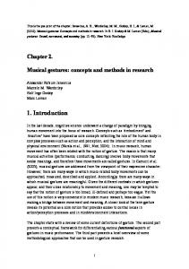
ABSTRACT It has been claimed that quantum mechanics is a non-local theory, i.e., that the predictions of quantum mechanics are at odds with a conception of the world where all the interactions are mediated by local mechanisms. The cited reason is the violation of the Bell inequality in cases where measurements are performed on quantum systems of particles that have interacted in the past. Quantum mechanics predicts that the state of the particles in such a system are correlated, a result obtained from considering a thought-experiment often known as EPR. In this thesis, I will argue that the violation of the Bell inequality in EPR forces us to either accept that causes sometimes act both backwards and forwards in time, or give up some widely-held assumptions about causal relations or the role of causal explanations. First, I will present three principles regarding causality that I take be widely accepted. I will then present the background for the claim the quantum mechanics is a non-local theory, and discuss the implications of non-local causal influences in light of the Special Theory of Relativity. One argument against a causal explanation of the EPR-correlations will be discussed, and different models for the causal structure of EPR will be assessed. I will argue that a retrocausal model – models that include instances of retrocausation, where the direction of causation is the opposite of the direction of time – is the only viable option if we want to uphold the three principles presented in chapter 1. I will discuss the plausibility of rejecting one of these principles, and argue that at least one of the can be restricted in a way that still accounts for our commitment to it. Finally, I will assess the non-local models against the retrocausal models, and argue that a retrocausal model offers interpretational advantages over the nonlocal alternatives.

V

VI

AKNOWLEDGEMENTS

I began writing this thesis in spring 2016. At that time, I only knew that I wanted to write something about quantum entanglement, a topic that has fascinated me since I first read about it in some popular science book when I was 15. I had long held the suspicion that this phenomenon would challenge some of our notions and beliefs about causality, and writing my thesis on the topic gave me the opportunity to explore this idea further. In going from this rough idea, I have benefitted greatly from the discussions with my two supervisors, Anders Strand and Øystein Linnebo. They have directed me towards relevant material, helped me organize my thoughts and opinions, and challenged me to provide greater clarity and better arguments. During these months, the shape of the thesis changed, as the possibility of retrocausation as an interpretation of EPR consistent with our causal intuitions grew from being an annoying problem for my intended argument into a possible conclusion. To see the thesis taking on a life on its own in this way, has proved to me that doing philosophy is something more than just finding arguments in support of pre-decided views. I want to thank The Science Studies Colloquium Series (Forum for Vitenskapsteori) for supporting my efforts. Their contribution made it possible for me to focus exclusively on the thesis in the final semester. Figures made with GeoGebra © 2017 International GeoGebra Institute

To Tomas and Linn, for seeing the errors that I didn’t. To my supervisors, for counsel and encouragement. To my parents, for always being there for me. To my friends, for bearing with me. To Henning Knutsen, who encouraged the curiosity of a young boy who wanted to make sense of a strange universe. VII

VIII

CONTENTS ABSTRACT .............................................................................................................................. V Aknowledgements ...................................................................................................................VII Contents .................................................................................................................................... IX 1

Introduction ........................................................................................................................ 1 1.1

Introducing the dialectic .............................................................................................. 1

1.2

‘Causality’ and Epistemic Practices ............................................................................ 1

1.2.1

Correlation and causality ...................................................................................... 1

1.2.2

Causal asymmetry and the direction of time ........................................................ 5

1.2.3

Absolute causal direction ..................................................................................... 8

1.3 2

3

Outline of the thesis ................................................................................................... 10

Quantum Mechanics and Locality.................................................................................... 12 2.1

The Einstein-Podolsky-Rosen Argument .................................................................. 12

2.2

The principle of local causality and the factorization condition ............................... 15

2.3

The EPR argument revisited ...................................................................................... 17

2.4

Local causality and Bell-type inequalities ................................................................. 20

2.5

Bell’s conclusion and the way forward ..................................................................... 24

The Principle of Relativity and Lorentz-invariance ......................................................... 25 3.1

What the Special Theory of Relativity doesn’t say ................................................... 25

3.2

A brief introduction to the Special Theory of Relativity ........................................... 26

3.2.1

The Special Principle of Relativity and the Galileo Transformations................ 26

3.2.2

The two postulates of the Special Theory of Relativity and the Lorentz

transformation .................................................................................................................. 28 3.2.3 3.3 4

The Minkowski spacetime and the light cone .................................................... 30

What the Special Theory of Relativity does say........................................................ 33

Causal Explanations and Causal Structures ..................................................................... 37 4.1

The argument thus far and where to go next ............................................................. 37 IX

4.2

4.2.1

Philosophical accounts of causality and CAUSAL EXPLANATION ............... 38

4.2.2

Indistinctness and non-separability .................................................................... 41

4.3

5

Causality as systematic correlations .......................................................................... 38

Causal Models of EPR ............................................................................................... 44

4.3.1

Local common cause models ............................................................................. 44

4.3.2

Non-local causal models .................................................................................... 46

4.3.3

Retrocausal models ............................................................................................ 48

Philosophical Implications of Bell’s Theorem ................................................................. 53 5.1

Taking stock .............................................................................................................. 53

5.2

Causal explanation and the screening-off criterion ................................................... 53

5.2.1

The importance of the screening-off criterion .................................................... 53

5.2.2

Arguments against the screening-off criterion ................................................... 55

5.3

Asymmetry on a non-local causal model .................................................................. 59

5.4

Argument for a retrocausal model ............................................................................. 62

5.5

Recent developments ................................................................................................. 65

5.6

Conclusion ................................................................................................................. 67

References ................................................................................................................................ 70

Figure 1: All the events (points) are a part of a shared causal structure. An arrow marks a direct causal connection between two events.. .................................................................... 3 Figure 2: A causal structure with a causal ordering. The structure has an overall direction, given by the increasing number of branches. ....................................................... 7 Figure 3: A causal structure with a causal loop. ................................................................... 8 Figure 4: The set-up of the thought-experiment EPR. cλ is the creation event, sA and sB are setting events, and mA and mB are measurement events. ............................................. 13 Figure 5: The only possible common causes for the events A and B are events in the overlap of the two light cones ................................................................................................ 16 Figure 6: The velocity of the ball relative to two different inertial frames that move relative to each other .............................................................................................................. 28 X

Figure 7: The light cone depicted in a three-dimensional spacetime ................................ 32 Figure 8: A possible causal structure in one reference frame ............................................ 34 Figure 9: There are infinitely many possible spacelike hyperplanes (here illustrated by coloured circles), some of which are simultaneity slices in the given reference frame .... 35 Figure 10: A collapse model for EPR. .................................................................................. 42 Figure 11: The Complex Common Cause Model, where the common cause-structure is uncertain. ................................................................................................................................ 45 Figure 12: The Hyperplane Model, where the common cause is a spacelike hyperplane prior to both measurement events ........................................................................................ 46 Figure 13: The Remote Outcome Dependence Model, where there is a causal connection between the measurement events at each wing (possibly through some outcome event in the path of the second particle) ............................................................................................. 47 Figure 14: The Remote Setting Dependence Model, where the outcome on one wing depends on the setting on the other wing. ............................................................................ 47 Figure 15: The Outcome Dependent Retrocausal Model, where the outcome at one wing has a causal influence on some event(s) in the past of the creation event (or possibly the creation event itself), which in turn is causally connected with the outcomes. ................. 48 Figure 16: The Setting Dependent Retrocausal Model, where the setting events has a causal influence on some event(s) in the past of the creation event (or possibly the creation event itself), which in turn is causally connected with the outcomes. ................. 49 Figure 17: Possible causal structure of EPR. The solid arrows mark the causal dependencies that are given, whereas the dotted arrows are possible causal dependencies. The red arrow connects the two outcomes, and the blue one outcome and the distant setting. In either case, either the Causal Markov Condition or the Causal Faithfulness Condition fails. .................................................................................................. 66

XI

XII

1 INTRODUCTION 1.1 INTRODUCING THE DIALECTIC The dialectic of this thesis will be based on the following three principles: CAUSAL EXPLANATION If any two distinct events, A and B, are systematically correlated, then there is a causal explanation for this correlation. TEMPORALITY

Causal and temporal asymmetry are related.

ABSOLUTENESS

The direction of causation is absolute.

These are epistemic claims: As I will argue in the next section, they capture certain features of ‘causality’ as it is incorporated in our description of reality and applied in our epistemic practices. However, the success of these practices is often taken to justify a further metaphysical commitment: That the principles represent facts about the `underlying´ causal structure of reality and the nature of causation. The central argument of this thesis is that this commitment requires us to accept the existence of retrocausation, i.e., that causes, in some cases, act both backwards and forwards in time. This follows from applying the principles to a phenomenon known as “quantum entanglement”, which I will argue either entails that future events have a causal influence on the past, or that causes act between spacelike separated events. I will show that the latter option entails that either TEMPORALITY or ABSOLUTENESS must be rejected, given the results of the Special Theory of Relativity. Rejecting retrocausation would thus require us to relax our metaphysical commitments, but I will argue that the perspectivalist view on the direction of causation offers one way of rejecting ABSOLUTENESS in a way that is consistent with its application in our epistemic practices.

1.2 ‘CAUSALITY’ AND EPISTEMIC PRACTICES 1.2.1 Correlation and causality CAUSAL EXPLANATION captures a common schema of reasoning: Whenever we observe two or more co-occurring events, we tend to look for causal explanation to account for this co-incidence. We notice that a lightning bolt is usually followed by thunder, and are lead to believe that there is some causal explanation for this fact. In Norse mythology, the god Thor 1

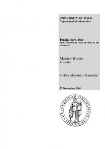
was assumed to be responsible for both, while we in modern times believe that it is a transmission of electrons between the ground and the sky that cause photons to be emitted and create the pressure wave we register as sound. However, as we also experience in our daily lives, sometimes strange coincidences occur by mere chance: A lot of famous people died the same year as Donald Trump was elected president of the United States, but it is unlikely that these events have any common cause(s)1. On the other hand, if Trump is re-elected in 2020, and this year also has a high celebrity mortality rate, we may start to suspect that these events are causally related in some way. Even more so if we develop a rigorous scientific theory which relates celebrity-deaths and the life of Donald J. Trump. Thus, by describing two events as systematically correlated, I mean that there must be a statistical correlation between the two types of events that is robust both empirically and theoretically. That is, it should be theoretically predicted (by a wellestablished theory) that 𝑃(𝐴, 𝐵) > 𝑃(𝐴) ∗ 𝑃(𝐵)2, and this prediction should be confirmed by observations.3 Furthermore, the events under considerations must be distinct. Otherwise, a causal explanation generally isn’t required, as there then is another explanation more readily available. For instance, the fact that a rose is red is systematically correlated with the fact that it is coloured, but this is because the former follows analytically from the latter, not because they are causally related. Rather than committing to a general theory of ‘explanation’, I will proceed on the assumption that a causal explanation would in part involve providing a description – a model – where the two events are a part of a shared causal structure (in which causal relations obtain between the relata in this structure), like what is illustrated in Figure 1. Furthermore, even though systematic correlation is a relation that obtains between types of events, I will assume that a causal explanation of these systematic correlations must involve causal relations between event-tokens. This would follow given the assumption that causal structures with event-types as relata supervene on causal structures where the relata are event-tokens.4 Otherwise, it is

1

There is of course the possibility that there are complex historical causes to both the rise of right-wing populism in America and the birth of celebrities at the right age for dying in 2016, but for the sake of the example we ignore this possibility. 2 𝑃(𝐴, 𝐵) is to be read as «the probability of A and B», whereas 𝑃(𝐴, 𝐵 | 𝐶) is to be read as «the probability of A and B, given C». 3 Empirically, the event-types A and B are correlated when the relative frequency of the event-tokens 𝑎1 , 𝑎2 , … and 𝑏1 , 𝑏2 ,…, of the event-types A and B respectively, display the relationship 𝑟𝑓((𝑎 , 𝑏)’𝑠) > 𝑟𝑓(𝑎’𝑠) ∗ 𝑟𝑓(𝑏’𝑠). 4 Note that this causal structure differs slightly from the concept of a ‘causal structure’ that is used in Bayes nets theories, as the relata in this latter framework are variables, where I assume the relata to be event-tokens.

2

possible to develop the argument with causal explanations in terms of types rather than tokens, given some account of how these event-types are instantiated at particular points in spacetime. For brevity, I will – following Tim Maudlin – say that events that are a part of such a structure are causally implicated with one another (Maudlin, 2002, pp. 128-129). This is intended as a rather weak notion, which neither distinguishes causes and effects nor exclusively applies to events in which one is the cause of the other. Accordingly, a causal explanation would – minimally – involve a claim to the effect that the events are causally implicated with one another; a fuller explanation would also involve a description of exactly how they are causally implicated.

Figure 1: All the events (points) are a part of a shared causal structure. An arrow marks a direct causal connection between two events..

Events can be causally implicated in two ways: They can be causally connected, in which case one event causes the other, possibly through some intermediaries. For example, the shattering of the window and the rock striking the glass are causally connected. In the figure, two events are causally connected if it is possible to trace the arrows (respecting their direction) from one event to the other.5 For instance, F and I are causally connected. Otherwise, two events can be causally implicated due to being causally connected to some shared common cause. Smoke and flames are causally implicated due to the exothermic reaction between the organic molecules in the kindling and the oxygen in the air, precipitated by extra addition of heat, which causes both release of photons (“flames”) and the release of

5

This is known as a directed path in the literature on causal Bayes nets. See e.g. Spirtes et al. (1993, pp. 25-31)

3

gases (“smoke”). In this case, the two events are causally implicated due to being causally connected with the same common cause(s). In the figure, the two events and the common cause will form a `fork´, where two arrows originating in the common cause point towards each effect.6 For instance, H and I are causally implicated due to the common cause A. CAUSAL EXPLANATION is inspired by Reichenbach’s principle of the common cause, which states that “if an improbable coincidence has occurred, there must exist a common cause” (Reichenbach, 1956, p. 157). “Improbable coincidences” would refer to the sort of events which in my terminology are systematically correlated, and causally implicated through the common cause(s). A further issue is what sort of conditions must apply to this common cause(s) for it to explain the correlation of its effects. Following Reichenbach, I suggest that a plausible condition is that conditional on the common cause(s) C, the effects A and B should be mutually independent, i.e., conditioning on the disjunction of the full list of common causes should screen off the correlation between A and B. From this it follows that C is the (full list of) common cause(s) of A and B only if the following applies:

Screening-off

𝑃(𝐴 |𝐵, 𝐶) = 𝑃(𝐴|𝐶) 𝑃(𝐵 |𝐴, 𝐶) = 𝑃(𝐵|𝐶)

{

If there is more than one common cause, C is taken to be the disjunction of these common causes (Reichenbach, 1956, pp. 159-160). The screening-off criterion captures the intuition that when two events are correlated due to some common cause(s), the correlation disappears when the common cause(s) are taken into account. The rationale behind it is the idea that events that aren’t causally implicated with each other are also statistically independent. If the events aren’t causally connected, any statistical dependence between two events must consequently be due to the common cause(s). The common cause(s) should explain away the correlation, so that statistical independence is restored when we control for them. A residual correlation would be an indication that we haven’t be able to identify all the common causes, and therefore not provided a full causal explanation of the correlation. For instance, life expectancy might be correlated with sneakers ownership. However, few will claim that sneakers ownership by itself causes people to live longer lives; we don’t live longer 6

I.e. there is an undirected, but not a directed path, joining the three events.

4

by simply buying a pair of sneakers and throwing them into the attic. Rather, we believe that the explanation is some common cause of both longer life expectancy and sneakers ownership, and it is tempting to think that the common cause is regular exercise. Then, we also expect that the correlation between sneakers ownership and life expectancy will disappear when we only look at the people who exercise regularly (some of them owning sneakers, whereas others do not). Accordingly, CAUSAL EXPLANATION involves two distinct claims: (a) That systematic correlations should be explained in terms of causal structure, and (b) that the correlation between two events should disappear conditional on their common causes. As such, CAUSAL EXPLANATION is closely related to the Causal Markov Condition: The Causal Markov Condition (CM) For all distinct variables X and Y in the variable set V, if X does not cause Y, then P(X | Y, Parents(X)) = P(X | Parents(X)). (Hausman and Woodward, 1999, p. 523) The Causal Markov Condition is treated as an axiom in the theory of causal Bayes nets developed partly in Spirtes et al. (1993), which has become part of the methodology in many sciences that work with statistical data (Näger, 2016, p. 1129).

1.2.2 Causal asymmetry and the direction of time Causes tend to precede their effects. Most – if not all – observations suggest that the direction of causation coincides with the direction of time. Even if this does not hold universally, it seems difficult to conceive of a direction of time without in some way relating it to a causal asymmetry (or vice versa): If time didn’t have a direction, how could we distinguish between causes and effects; and if there were no causal asymmetry, how could the progression of events have any direction? Empirically as well as conceptually, causal and temporal asymmetry seem to be closely related. Though the above statement is hard to deny, there are different accounts for the exact nature of this relation. One view, at least dating back to Hume, is that the difference between cause and effect is simply that the former occurs before the latter: The conceptual connection between the direction of time and causal asymmetry is due to our tendency to assume that when two events occur in constant conjunction, the earlier event is the cause of the later event (Hume, 1739, pp. 378, 388). On this view, known as the temporal theory on the direction of causation (Dowe, 2000, p. 179), causal asymmetry is defined by temporal priority: For two 5

causally connected events, x and y, x is a cause of y iff x occurs before y. This also ensures that the causal relation has a direction, at least to the extent that time has one. Hence, TEMPORALITY can be restated as: STRONG TEMPORALITY The direction of causation is the direction of time. The motivation I have described for this principle may be called conventionalist, in the sense that the asymmetry of causation is defined in terms of a convention, where we label the earlier event “cause” and later event “effect” (Price, 1996, pp. 136-138). On the conventionalist account, retrocausation – where a later event causes an earlier event – is, by definition, impossible. However, a non-conventionalist may also ascribe to this principle. In that case, the non-existence of retrocausation is a contingent fact about our world, but not a conceptual impossibility. On the other hand, a non-conventionalist might also not want to rule out retrocausation in our world, in which case one might want to adopt a weaker principle (given below). A reason to object to the temporal theory is that one finds the direction of time just as, if not more, mysterious than the direction of causation. One might therefore think that the direction of time should be analysed in terms of causal asymmetry, rather than the opposite. See e.g. Reichenbach (1956) for a comprehensive attempt at a causal theory of time. This theory takes causal asymmetry as its starting point, and reduces temporal ordering to causal ordering (causal asymmetry itself might be defined in terms of some other physical asymmetry, or be taken as a primitive fact about reality). To avoid preconception about the directionality of time, this ordering can be defined in terms of a betweenness-relation (Reichenbach, 1956, pp. 32-33): If A causes B and B causes C, then B is causally between A and C. The betweennessrelation is non-directional in the sense that if B is between A and C, it is also between C and A. It is also transitive: If B is between A and C, and C is between B and D, then B is between A and D. For a given system, we can define a causal ordering by listing the betweennessrelations. This will give us a (weak) partial ordering for the system. Now, the claim is that if an event B is causally between A and C, it is also temporally between A and C. For such an account, TEMPORALITY can be restated as: WEAK TEMPORALITY

The temporal ordering of a system is the same as the causal ordering of the system

Note that this follows from STRONG TEMPORALITY: If A causes B, B causes C, and the direction of causation is the same as the direction of time, it follows that B is after A and C is 6

after B, so B is temporally between A and C. Unlike STRONG TEMPORALITY, however, this principle is compatible with the possibility of retrocausation: If A causes B, and B causes C, B is causally and hence temporally between A and C. This will be the case even if the direction of causation is the opposite of the direction of time, i.e., if C occurs before B, which occurs before A. To see how this principle can be used to define a direction of time, we can consider the causal structure depicted in Figure 2.

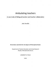
Figure 2: A causal structure with a causal ordering. The structure has an overall direction, given by the increasing number of branches.

This structure has an overall direction that can be defined in terms of the increasing number of branches. The structural asymmetry might be due to some other physical asymmetry, as the entropic increase in the universe stated by the second law of thermodynamics (assuming certain boundary conditions), or the Kaon arrow (Dowe, 1992, pp. 189-191). It is then possible to use this asymmetry to define a direction of time, for instance by associating the future-direction with increased branching: Since E is temporally between F and C, it lies in the past of F and the future of C. Since C is temporally between A and E, it lies in the past of E and the future of A. Consequently, A occurs before C, which occurs before E, which occurs before F. Where no arrow connects two events, the temporal ordering is indeterminate, and might vary in different reference frames (see chapter 3 on the Special Theory of Relativity). In the case of retrocausation, we have a causal loop in the structure. For these systems, we cannot use the betweenness-relation to define a causal ordering, since any event is between any other two events. Nevertheless, an event that is a part of a causal loop might still lie in the future of another event in that causal loop, due to being between this event and another event that lies outside the loop. See for example Figure 3: Here B is between A and G, and 7

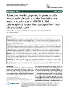
accordingly lies in the future of A and the past of G. This is consistent with it being between A and C, even if A is also between C and B: Causal loops do not have a temporal ordering, so any temporal ordering must be due to the event partaking in betweenness-relations outside the causal loop, like B in Figure 3.

Figure 3: A causal structure with a causal loop.

Depending on the account for causal and temporal asymmetry you accept, TEMPORALITY can thus be interpreted as both allowing for or rejecting the possibility of causal loops. This will be relevant for our discussion in chapter 4. In the following discussion on non-local correlations in quantum mechanics, both the strong and the weak version of TEMPORALITY will be evaluated.

1.2.3 Absolute causal direction ABSOLUTENESS is the claim that the direction of causation for two causally connected events is not relative to the observer, perspective, reference frame, context, etc. In extension, any two observers, even employing different reference frames, should be able to agree on which event causes the other. It follows that the same should apply to the causal ordering of a system, as defined in the previous section. Later in this thesis, I will show that this claim is tantamount to the demand that the causal ordering should be Lorentz invariant (see chapter 3). The directionality of the causal relation is required by the causal theory of time I sketched in the previous section: In order to define a direction for the causal structure in terms of increased branching, it is necessary to assume that a common cause of two events cannot lie causally between the events. Otherwise, ignoring the direction of the causal relation entirely, 8

almost any path through the causal structure depicted in Figure 2 would correspond to an increase in number of branches, and there would be no structural asymmetry that could be used to define a direction of time. Given that this structural asymmetry is absolute in the sense stated above, the direction of causation, and therefore also causal ordering, must be so too. It follows that rejecting an absolute direction of causation would require us to abandon a causal theory of time of the sort sketched in the previous section. ABSOLUTENESS is furthermore motivated by the desire to include causal explanations in our scientific theories: Whether it is the fusion of hydrogen atoms that cause a release of highenergy photons or the release of high-energy photons that cause the fusion of hydrogen atoms isn’t a matter of perspective. A minimal requirement for any scientific account of the given phenomena is that it is invariant under change of reference frame or context7, and this should apply to causal accounts as well. Bertrand Russell argues, to the contrary, that causal explanations have no part in a scientific account of the world. He notes that the concept ‘cause’ does not generally appear in the contemporary scientific literature, and further argues that (most of) the laws of fundamental physics are time-symmetric, whereas causation is generally believed to be asymmetric (Russell, 1912, p. 26). Russell here ignores the fact that fundamental physics is more than a set of laws. Fundamental physics also incorporates idealised models, illustrations and physical descriptions of the phenomena under study. Typically, both when doing text-book exercises and when making predictions to be tested, physicists create idealised models where the different causal relations are specified, and employ the appropriate differential equations that express the general physical laws in order to make predictions. These predictions are then tested against observations. Furthermore, it is often the idealised models, and not the laws themselves, that are tested. If we think that the models are idealised representations of absolute, non-perspectival features of reality, then it follows that the causal account they include are so too. This point can reasonably be extended to non-scientific explanations: When we ask why there is a foul stench emanating from the refrigerator we expect the explanation – that our roommate has brought in some fancy, smelly cheese from their latest trip to France – to apply no matter what context the claim is evaluated in. Furthermore, part of coming up with

7

A similar idea also motivates the Special Principle of Relativity, which will be discussed in chapter 3, that states that all physical laws should have the same formulation in all inertial frames.

9

effective strategies (Cartwright, 1979) to address the situation at hand – demand that the roommate removes the smelly cheese from the common area – requires that the causal explanation display some form of asymmetry. Otherwise we could hope to conjure up fancy cheese by stinking up the fridge. Similarly, when the health department releases a campaign against smoking as a cancer-preventing program, rather than treating people with cancerpreventing drugs to make them quit smoking, it is the asymmetry of the causal relation that accounts for the fact that the former is an effective strategy, whereas the latter isn’t. In the interest of ensuring that the campaign is universally applicable (and well-spent use of the taxpayers’ money), we furthermore demand that the strategy is based on some objective, person-independent facts about the relation between smoking and cancer. Hence, it seems that the asymmetry of the causal relation is crucial both if causal explanations should be included in our scientific theories, and in our practical use of causal concepts. Furthermore, the application of causal asymmetry to widely different contexts and on large scopes, suggests a commitment to the assumption that it is an absolute, non-perspectival feature of reality.

1.3 OUTLINE OF THE THESIS In this chapter, I presented the three principles that will form the basis for the dialectic of this thesis, and discussed the role they have in our epistemic practices. In the following chapters I will discuss the implications of applying them to a certain phenomenon described by quantum mechanics. The EPR-argument will be presented in chapter 2. This argument describes a phenomenon known as “quantum entanglement” – where quantum mechanics predicts that the outcomes of measurements performed on certain two-particle systems are correlated – and provides a context for the following derivation of the Bell inequality. I will demonstrate that the predictions of quantum mechanics violate the Bell inequality, and show how this led to the conclusion that the EPR-correlations had to be explained by non-local influences. In chapter 3, I will discuss the implications of non-local causal influences in light of the Special Theory of Relativity, and argue that this entails a rejection of either TEMPORALITY or ABSOLUTENESS. I will also address some common misconceptions regarding the possibility of superluminal influences. Though important for a full understanding of the issue, 10

chapter 2 and chapter 3 are rather technical. The conclusions drawn in these chapter will be summarized in beginning of chapter 4, so it is possible to skim through these parts of the thesis. In chapter 4, I will consider whether a causal explanation of EPR follows from some traditional theories on causation. I will also address a common objection to the claim that the EPR-correlations require a causal explanation. Next, I will consider some different models for a causal structure that can explain the EPR-correlations, and argue that a commitment to CAUSAL EXPLANATION, TEMPORALITY and ABSOLUTENESS requires us to accept a retrocausal model. Finally, in chapter 5, I will explore the option of rejecting one of the principles. First, I will discuss some arguments against the screening-off criterion that is assumed by CAUSAL EXPLANATION, and consider one way that ABSOLUTENESS can be restricted that still justifies its application in our epistemic practices. This admits a non-local causal model of EPR, which will be evaluated against a retrocausal model.

11

2 QUANTUM MECHANICS AND LOCALITY 2.1 THE EINSTEIN-PODOLSKY-ROSEN ARGUMENT The Einstein-Podolsky-Rosen argument (EPR) was first put forward in an issue of Physical Review from 15. May 1935, co-authored by Albert Einstein, Boris Podolsky, and Nathan Rosen (Einstein et al., 1935). The purpose of this argument was to show that the orthodox interpretation of quantum mechanics was incomplete. I shall first give a summary of the argument, and then go give a more detailed description. Initially, the argument sets out to provide a condition for a theory (or a description of the world) to be complete: A description is complete iff nothing that is an “element of reality” is left out of that description (Einstein et al., 1935, p. 777). As far as we know, no theory or description of the world that we currently have is complete in this sense, as the only way we can establish this is first by identifying every single “element of reality”, which is an enormous demand to place on our current theories. However, this is not required for EPR to work: What is required is to show we can find some “elements of reality” that are left out by quantum mechanics. Hence, we need a sufficient condition for something being an element of reality, and EPR provides us with the following “criterion of reality”: […] if, without in any way disturbing a system, we can predict with certainty (i.e., with probability equal to unity) the value of a physical quantity, then there exists an element of reality corresponding to this quantity. (Albert, 1992, pp. 61-62) To illustrate this, we might consider one way to measure the mass of a planet: If the planet has a satellite orbiting it, then we can measure the period 𝑃 and the radius 𝑟 of this orbit. From classical mechanics, we can then approximately predict the mass of the planet as: 4𝜋 2 𝑟 3 𝑀= 𝐺 𝑃2 Thus, without disturbing the system, we can predict the mass of the planet, and this physical quantity is an “element of reality”. The argument then goes on to show that quantum mechanics itself is able to predict the values of some physical quantities that are left out of the quantum state describing the system. Since, on the orthodox interpretation of quantum mechanics, the quantum state is a complete 12

description of the system (Griffiths, 2005, pp. 2-5), a contradiction occurs: If, per the orthodox interpretation, the quantum-mechanical description is complete, it follows that there must be some elements of reality that are not part of this description. Hence, the quantummechanical description is incomplete. Now, let us delve into the details. The rest of the argument involves a particular thoughtexperiment where a composite quantum-mechanical system is prepared in some particular state, and the two individual members of this system are sent to two different measuring devices. I will use “EPR” to refer to both this thought-experiment as well as the original argument. See below for illustration:

Figure 4: The set-up of the thought-experiment EPR. cλ is the creation event, sA and sB are setting events, and mA and mB are measurement events.

In what follows, rather than presenting the original form of the argument, I shall present David Bohm’s version of it (Fine, 2016). In this particular example, we take the composite state at the source to be two electrons in a singlet-state. This state can be given the following specification: |𝜑 ⟩ =

1 √2

(|↑1𝜃 ⟩|↓2𝜃 ⟩ − |↓1𝜃 ⟩|↑2𝜃 ⟩)

Equation 1: The singlet state

The arrows mark the different spin-orientation of the particle 1 and 2 along the axis theta. On the standard interpretation, this state is a complete description of the system before performing an experiment. This is what is meant by the electrons being in an “entangled state”.

13

The probability that we will measure the system in the state |↓1𝜃 ⟩|↑2𝜃 ⟩ is given by the Born rule (Harris et al., 2016, pp. 1,3): 𝑃(|↓1𝜃 ⟩|↑2𝜃 ⟩) = |⟨𝜑| ↓1𝜃 ⟩|↑2𝜃 ⟩|2 =

1 2

and similarly for measuring the system in the state |↑1𝜃 ⟩|↓2𝜃 ⟩. The probability for measuring the system in |↑1𝜃 ⟩|↑2𝜃 ⟩ or |↓1𝜃 ⟩|↓2𝜃 ⟩ is zero. The individual probabilities of measuring one of the particles in any particular spin-state will then be: 𝑃(↑1𝜃 ) = 𝑃(↓1𝜃 ) = 𝑃(↑2𝜃 ) = 𝑃(↓2𝜃 ) =

1 2

Before performing the experiment, we can only predict that we will measure a particular spin on an individual particle 50% of the time. The two particles are sent to the measuring devices A and B, and the two devices measure the spin along a particular axis perpendicular to its flight path. If the devices are set to measure the spin along the same axis, by conservation of momentum, the spin of the two particles will be anti-correlated. Thus, we can find the conditional probabilities: 𝑃(↑2𝜃 | ↓1𝜃 ) = 1 𝑃(↑2𝜃 | ↑1𝜃 ) = 0 Thus, by measuring the spin of particle 1, we can predict with certainty that the spin of particle 2 will be the opposite. Since the measuring devices can be separated either by distance or by some other means, we will have predicted the outcome of a measurement on particle 2 without in any way disturbing the system. Thus, by the “criterion of reality”, the spin of particle 2 is an element of reality. However, a complete description of reality should then contain the spin of particle 2, which is left out by the original singlet-state. The upshot of this argument is that the singlet-state cannot be a complete description of the composite system. Barring any direct influence from one wing of the experiment to the other, the only explanation of the correlations predicted by quantum mechanics would be that each particle had a determinate state at the outset (Maudlin, 2002, pp. 139-140). This entails that there must be some so-called “hidden variables” in addition to the standard quantum state, which would allow one to predict the results of each experiment. One might then try to develop such a hidden variable-theory consistent with the result of standard quantum mechanics. However, in 1964 John S. Bell released a paper in which he proved that no such 14

theory is possible (Bell, 1964). More than this, however, Bell’s results challenges more fundamental notions of a world governed by local causal influences. In the following sections, I will give an account of the principle of local causality (PLC), and demonstrate how it plays a part in the EPR-argument. Furthermore, I will use this principle to derive a version of the Bell inequality, and show that the predictions of standard quantum mechanics violate this inequality.

2.2 THE PRINCIPLE OF LOCAL CAUSALITY AND THE FACTORIZATION CONDITION

A crucial part of the EPR-argument is the assumption that the measurement at one wing of the experiment cannot influence the particle at the other wing. Even though the composite quantum state contains all the information about the system quantum mechanics can offer us, each particle is supposedly localized at each wing of the experiment prior to measurement, and the act of measuring the spin of one particle is a localized event. Each wing of the experiment has some `reality´ pertaining to it, and what happens to the `reality´ of one wing, is in some manner barred from having any influence on the `reality´ of the other wing. This sort of restriction of the possible influences between the realities of the two separated composites of the system is known as “locality”. There are many ways of defining locality, corresponding to different ontologies (i.e., whether what you consider to be `real´ are events, particles, observables, states, etc.), ways of separating these things (i.e., by distance or some sort of impenetrable barrier), and sorts of influences (causal, energy transmission, signals, information, etc.). In what follows, we will consider the form of locality as formulated by John S. Bell, which led to the derivation of the Bell inequality. In his 1975 paper, The Theory of Local Beables, John S. Bell gives his account of what he terms “The Principle of Local Causality” (Bell, 1975, pp. 1-2): For any spatio-temporally localized event8 A, the possible causes of A will be within the backwards light cone of A. If two events A and B are outside each other’s backwards light cones, neither can be a cause of

Rather than committing to a particular ontology, Bell uses “beable” to as a generic term for any sort of thing that has some claim to be a part of physical reality: It includes fields, objects, energy, etc. (Bell, 1975, p. 1) When I define local causality in terms of events, it is simply because this term lends itself well to the discussion, and should not be taken as an ontological commitment. 8

15

the other. Furthermore, the possible common causes of A and B will be within the overlap of the backwards light cones of A and B. See Figure 5.

Figure 5: The only possible common causes for the events A and B are events in the overlap of the two light cones

It is important to note that this principle assumes that the `realities´ – “beables” in Bell’s terminology, “events” in mine – of A and B are themselves local. They need not be: Total energy of a system is an example of a non-local beable. This is relevant, for it is possible to challenge the claim that the `reality´ of the quantum state of each particle is localized to a particular spatio-temporal region. In that case, PLC might not apply, as it might not be a genuine causal relation. For now, however, we will leave these difficulties aside. In order to make principle relevant to the predicted correlations of EPR, we need some way of relating the causes and correlations. This is achieved by the screening-off criterion, which was formulated in chapter 1 as: Screening-off

𝑃(𝐴 |𝐵, 𝐶) = 𝑃(𝐴|𝐶) 𝑃(𝐵 |𝐴, 𝐶) = 𝑃(𝐵|𝐶)

{

By applying standard probability theory, we find that this is equivalent to 𝑃(𝐴, 𝐵|𝐶) = 𝑃(𝐴|𝐶) ∗ 𝑃(𝐵|𝐶).9 From these two assumptions (i.e., the screening-off criterion and PLC), Bell is able to derive what is known as the factorization condition: We let SA be all the events within the backwards

9

By standard probability theory, 𝑃(𝐴, 𝐵| 𝐶) = 𝑃(𝐴|𝐵, 𝐶) ∗ 𝑃(𝐵|𝐶). Using the screening-off criterion, we find 𝑃(𝐴, 𝐵|𝐶) = 𝑃(𝐴|𝐶) ∗ 𝑃(𝐵|𝐶).

16

light cone of A, but not B; SB be all the events within the backwards light cone of B, but not A; and C be all the events within the overlap of the two light cones (see Figure 5). Then: FACTORIZATION

𝑃(𝐴, 𝐵 | 𝑆𝐴 , 𝑆𝐵 , 𝐶) = 𝑃(𝐴 | 𝑆𝐴 , 𝐶) ∗ 𝑃(𝐵 | 𝑆𝐵 , 𝐶)

By way of the screening-off criterion, we express PLC in a way that allows us to evaluate whether or not a particular theory obeys this principle: On this notion of locality, any theory which determines joint probability functions consistent with FACTORIZATION, will be a local theory. In the next section, I will show how the factorization condition is assumed in the EPR-argument, and in the following section I will demonstrate how Bell used it to argue that quantum mechanics is a non-local theory.

2.3 THE EPR ARGUMENT REVISITED To see how this applies to our previous discussion on the EPR argument, we may return to our illustration (Figure 4). In this simplified thought-experiment, there are only five distinct events to consider: I.

II. III. IV. V.

A creation event cλ, where the composite quantum state λ is created, and the individual components are sent in different directions. At this point, we have made no assumption as to what type of state this is: It might be the indeterminate state of the standard interpretation, or a determinate state with hidden variables. A setting event 𝑠𝐴 of measuring device A. A setting event 𝑠𝐵 of measuring device B. A measurement-event 𝑚𝐴 at device A. A measurement-event 𝑚𝐵 at device B.

We further assume that we can set the measuring devices to measure the spin along three different directions. The aim of this section is to reformulate the EPR-argument in more formal terms by using the factorization condition, as well as introduce some notation that will be useful later. We first lay down some general requirements: An empirical theory of this system should aim to determine some joint probability functions of the form 𝑝𝜆𝐴𝐵 (𝑥, 𝑦|𝑖, 𝑗)10, where 𝑥, 𝑦 are the outcomes of the measurement (spin up or spin down), and 𝑖, 𝑗 = 1, 2, 3 are the different settings for each measuring device (the axis along which we measure the spin).

The notation and discussion in the following paragraphs are heavily influence by Jon P. Jarrett in Bell’s theorem: A guide to the implications. See Jarrett (1989, pp. 65-69). 10

17

As probability functions, 𝑝𝜆𝐴𝐵 must obey the following constraints: 0 ≤ 𝑝λ𝐴𝐵 (𝑥, 𝑦|𝑖, 𝑗) ≤ 1 ∑ ∑ 𝑝λ𝐴𝐵 (𝑥, 𝑦|𝑖, 𝑗) = 1 𝑥

𝑦

Furthermore, we can define the marginal and conditional probabilities: 𝑝λ𝐴 (𝑥|𝑖, 𝑗) ≝ ∑ 𝑝λ𝐴𝐵 (𝑥, 𝑦|𝑖, 𝑗) 𝑦

𝑝λ𝐵 (𝑦|𝑖, 𝑗) ≝ ∑ 𝑝λ𝐴𝐵 (𝑥, 𝑦|𝑖, 𝑗) 𝑥

𝑝λ𝐴 (𝑥|𝑖, 𝑗, 𝑦)

𝑝λ𝐴𝐵 (𝑥, 𝑦|𝑖, 𝑗) ≝ 𝑝λ𝐵 (𝑦|𝑖, 𝑗)

𝑝λ𝐵 (𝑥|𝑖, 𝑗, 𝑥)

𝑝λ𝐴𝐵 (𝑥, 𝑦|𝑖, 𝑗) ≝ 𝑝λ𝐴 (𝑥|𝑖, 𝑗)

Lastly, an asterisk will be used to indicate a nonmeasurement; for instance, 𝑝λ𝐴 (↑,∗ |1,∗) will be the probability of device A measuring the spin along the x-axis as up, when no measurement is performed by device B. We are now able to give a more precise articulation of the premises and conclusions underlying EPR. Firstly, EPR assumes local causality, which is captured in the factorization condition. Applied to our current example, this becomes: FACT.*

𝑝λ𝐴𝐵 (𝑥, 𝑦|𝑖, 𝑗) = 𝑝λ𝐴 (𝑥|𝑖,∗)𝑝λ𝐵 (𝑦| ∗, 𝑗)

EPR furthermore assumes standard quantum mechanics, which predicts that the spin of the two particles should be anti-correlated when the spin is measured along the same axis for both devices. Thus, we have: CONSERVATION

𝑝λ𝐴𝐵 (↑, ↑ |𝑖, 𝑖) = 𝑝λ𝐴𝐵 (↓, ↓ |𝑖, 𝑖) = 0

EPR argues from CONSERVATION and the principle of local causality that a complete state description would yield: DETERMINISM

𝑝λ𝐴𝐵 (𝑥, 𝑦|𝑖, 𝑗)𝜖{0,1}

18

i.e., that given the complete state description we could predict any outcome of a trial with any detector settings with certainty. To see this, we can write out CONSERVATION with FACT*. This gives us the following marginal probabilities: 𝑝λ𝐴 (↑ |𝑖,∗) = 0 𝑝λ𝐴 (↑ |𝑖,∗) = 0 𝑝λ𝐴 (↑ |𝑖,∗) = 1

𝑎𝑛𝑑 𝑎𝑛𝑑 𝑎𝑛𝑑

𝑝λ𝐵 (↑ | ∗, 𝑖) = 1 𝑝λ𝐵 (↑ | ∗, 𝑖) = 0 𝑝λ𝐵 (↑ | ∗, 𝑖) = 0

and similarly for 𝑝λ𝐴𝐵 (↓, ↓ |𝑖, 𝑖). Writing out the anti-parallel case, we find that: 𝑝λ𝐴𝐵 (↑, ↓ |𝑖, 𝑗) = 𝑝λ𝐴 (↑ |𝑖,∗)𝑝λ𝐵 (↓ | ∗, 𝑗) Since each of the two marginal probabilities are either 1 or 0, we find that the joint probability function is also either 1 or 0. In section 2.1 I claimed that this led EPR to conclude that the quantum mechanical state description cannot be the complete state. Now we see why this must be so: In the case were the settings on both detectors are the same (𝑖 = 𝑗), standard quantum mechanics predicts that 𝑝λ𝐴𝐵 (↑, ↓ |𝑖, 𝑖) = 𝑝λ𝐴𝐵 (↓, ↑ |𝑖, 𝑖) = 0.5, while we have found them to be either 0 or 1. By the “criterion of reality”, the complete description should contain the states of the individual particles. The next question is how this solves the apparent inconsistency in the predictions given by quantum mechanics. In the preceding argument, I assumed that the joint probability function given by quantum mechanics was 𝑝λ𝐴𝐵 (𝑥, 𝑦|𝑖, 𝑗). This is based on the standard interpretation, in which the singlet state is a complete description of the composite system, and there is no fact of the matter whether an electron has spin up or spin down prior to measurement. The theory can only assign probabilities to the outcomes; quantum mechanics is an indeterministic theory. I have shown how this led to apparent inconsistency. However, the preceding requirements – i.e., the factorization condition, the general requirements of an empirical theory, and standard probability theory – are compatible with both indeterministic and deterministic theories, i.e., theories that only give us the probability of an event occurring and theories that predict with certainty what event will occur. Hence, it might be possible that, by adding some unknown – and possibly unknowable – hidden variables to this state description, we can get both a deterministic theory and a complete description. Such “hidden variable theories” (HVT’s for short) would be able to predict with certainty the outcomes of the experiment given the correct and complete state 19

description. Still, there might be some uncertainty as to what the quantum state is in each trial of the experiment. Thus, the observed frequencies of the outcomes are due to variations of the quantum state from trial to trial, rather than the probabilistic nature of reality itself. A fullyfledged theory must also provide some probability density function 𝜌(λ) on the set of possible states Λ, that predicts how often a particular state occurs across the different trials. In general, the predicted relative frequencies of the outcomes are given by 𝑝 𝐴𝐵 (𝑥, 𝑦|𝑖, 𝑗) = ∫ 𝑝λ𝐴𝐵 (𝑥, 𝑦|𝑖, 𝑗)𝜌(λ)𝑑λ λϵΛ

where deterministic theories will assign 𝑝λ𝐴𝐵 (𝑥, 𝑦|𝑖, 𝑗) as either 0 or 1. These predictions are compared to the observed frequencies to assess our theory. If the quantum state is not the total state of the system, but there are hidden variables as well, then quantum mechanics only predicts the expectation value of the different possible total states, 𝑝 𝐴𝐵 (𝑥, 𝑦|𝑖, 𝑗) = ∫λϵΛ 𝑝λ𝐴𝐵 (𝑥, 𝑦|𝑖, 𝑗)𝜌(λ)𝑑λ, where each of the 𝑝λ𝐴𝐵 (𝑥, 𝑦|𝑖, 𝑗) is either 0 or 1. By tweaking the probability density 𝜌(λ) in our HVT we could hope to reproduce the quantum mechanical predictions. The question then is if there is any way of tweaking the probability densities so our HVT is consistent with standard quantum mechanics. Bell demonstrated that this was impossible: In fact, no local theory, i.e., no theory obeying the factorization condition, would be able to reproduce the quantum mechanical predictions. This will be the topic of the next section.

2.4 LOCAL CAUSALITY AND BELL-TYPE INEQUALITIES In the previous section I demonstrated how PLC entered into the EPR argument, and how we might get a theory which is both consistent with the predictions given by standard quantum mechanics, and the results when applying the factorization condition, by the addition of hidden variables. In this section, I will first give a general overview of Bell’s proof that no such theory is possible, and then go on to derive another version of this proof.

20

From the factorization condition and standard probability theory, Bell was able to derive his version of what has been known as the Bell inequality (Bell, 1975, p. 6): |𝑃(𝑠𝐴 , 𝑠𝐵 , 𝑐) ∓ 𝑃(𝑠𝐴 , 𝑠′𝐵 , 𝑐)| + |𝑃(𝑠′𝐴 , 𝑠𝐵 , 𝑐) ± 𝑃(𝑠′𝐴 , 𝑠′𝐵 , 𝑐)| ≤ 2 Equation 2: The Bell inequality

Here 𝑠𝐴 , 𝑠𝐵 , 𝑐 (primed or un-primed) are variables that specify the particular experimental setup (in the red, blue and green backwards light-cones respectively). After deriving this inequality in The Theory of Local Beables, Bell then proceeds to show that quantum mechanics violates it by considering a pair of photons created by a decaying neutral pion. For a particular experimental set-up, he is able to show that |𝑃(𝜃, 𝜎) − 𝑃(𝜃, 𝜎′)| + 𝑃(𝜃′, 𝜎) − 𝑃(𝜃 ′ , 𝜎 ′ ) − 2 = 2𝐾(√2 − 1) where K is a positive number determined by the creation mechanism. The important thing to note is that the right-hand side of this equation can be a positive (non-zero) number, in violation of the Bell inequality |𝑃(𝑠𝐴 , 𝑠𝐵 , 𝑐) ∓ 𝑃(𝑠𝐴 , 𝑠′𝐵 , 𝑐)| + |𝑃(𝑠′𝐴 , 𝑠𝐵 , 𝑐) ± 𝑃(𝑠′𝐴 , 𝑠′𝐵 , 𝑐)| − 2 ≤ 0 with 𝑠𝐴 = 𝜃, 𝑠𝐵 = 𝜎 and 𝑐 is the fixed specification of the creation mechanism. This led Bell to conclude that […] quantum mechanics is not embeddable in a locally causal theory as formulated above (Bell, 1975, p. 9) It might be of interest to see in which way the violation of the Bell inequality implies a violation of PLC. In what follows, I will therefore derive a Bell-type inequality to demonstrate how the factorization criterion enters into it. Rather than deriving Bell’s original inequality (Equation 2). I will instead derive a version known as the Bell-Clauser-HorneShimony-Holt inequality. The derivation is taken from Shimony (2016). Suppose that we have a complete state λ (with or without hidden variables), and that the settings on the two detectors are chosen independently. We further suppose that the outcomes (𝑥, 𝑦) of a measurement can either be 1 or -1 (corresponding to spin up and spin down)11. We then define the expectation value for both outcomes as:

11

There are variants of the theorem in which 𝑠 and 𝑡 can take any discrete values in the interval [-1, 1], but for our purposes this simplified version is enough. See Shimony (2016).

21

𝐸λ (𝑖, 𝑗) = ∑ ∑ 𝑝λ𝐴𝐵 (𝑥, 𝑦|𝑖, 𝑗) 𝑥𝑦 𝑥

𝑦

And similarly for any other settings (𝑖, 𝑗’), (𝑖’, 𝑗), (𝑖’, 𝑗’). By FACT* we can factorize 𝑝λ𝐴𝐵 (𝑥, 𝑦|𝑖, 𝑗), so that: 𝐸λ (𝑖, 𝑗) = ∑ 𝑝λ𝐴 (𝑥|𝑖)𝑥 ∑ 𝑝λ𝐵 (𝑦|𝑗) 𝑦 𝑥

𝑦

We then define: 𝑞 = ∑ 𝑝λ𝐴 (𝑥|𝑖)𝑥 ;

𝑞 ′ = ∑ 𝑝λ𝐴 (𝑥|𝑖′)𝑥

𝑥

𝑥

𝑟 = ∑ 𝑝λ𝐵 (𝑦|𝑗)𝑦 ;

𝑟′ = ∑ 𝑝λ𝐵 (𝑦|𝑗)𝑦 ;

𝑦

𝑦

so that 𝐸λ (𝑖, 𝑗) = 𝑞𝑟. Since 𝑥 and 𝑦 can take the values 1 and -1, and the probabilities 𝑝 can take some value between 0 and 1, the single expectation values 𝑞, 𝑞′, 𝑟 and 𝑟′ are constrained by the interval [1, 1]. We then observe that 𝑆 ≝ 𝑞𝑟 + 𝑞𝑟 ′ + 𝑞 ′ 𝑟 − 𝑞′𝑟′ will be constrained by the interval [2,2]. Hence: −2 ≤ 𝐸λ (𝑖, 𝑗) + 𝐸λ (𝑖, 𝑗′) + 𝐸λ (𝑖′, 𝑗) − 𝐸λ (𝑖′, 𝑗′) ≤ 2 Ex hypothesi, we do not know the complete state λ, but any HVT should provide a probability density 𝜌(λ) that allow us to test the theory empirically (see section 2.3). We define the expectation value for a given probability density function 𝜌 by: 𝐸𝜌 (𝑖, 𝑗) = ∫ 𝐸λ (𝑖, 𝑗)𝜌(λ)𝑑λ λϵΛ

From our previous result, we thus find: 𝐸𝜌 (𝑖, 𝑗) + 𝐸𝜌 (𝑖, 𝑗′) + 𝐸𝜌 (𝑖′, 𝑗) − 𝐸𝜌 (𝑖′, 𝑗′) = ∫(𝐸λ (𝑖, 𝑗) + 𝐸λ (𝑖, 𝑗′) + 𝐸λ (𝑖′, 𝑗) − 𝐸λ (𝑖′, 𝑗′))𝜌(λ)𝑑λ λϵΛ

Since 𝜌(λ) have values between 0 and 1, and we have ∫λϵΛ 𝜌(λ)𝑑λ = 1:

22

−2 ∫ 𝜌(λ)𝑑λ ≤ 𝐸𝜌 (𝑖, 𝑗) + 𝐸𝜌 (𝑖, 𝑗 ′ ) + 𝐸𝜌 (𝑖 ′ , 𝑗) − 𝐸𝜌 (𝑖 ′ , 𝑗 ′ ) ≤ 2 ∫ 𝜌(λ)𝑑λ λϵΛ

λϵΛ

−2 ≤ 𝐸𝜌 (𝑖, 𝑗) + 𝐸𝜌 (𝑖, 𝑗 ′ ) + 𝐸𝜌 (𝑖 ′ , 𝑗) − 𝐸𝜌 (𝑖 ′ , 𝑗 ′ ) ≤ 2 Equation 3: The BCHSH-inequality

Any local HVT will obey this inequality, and the claim is that standard quantum mechanics violates it. We can see this in the case of our singlet-state: The expectation value when we measure the spin of particle 1 and particle 2 along the different axes 𝑖 and 𝑗 is given by (Griffiths, 2005, p. 424): 𝐸𝜑 (𝑖, 𝑗) = − cos 𝜃 𝜋

Where 𝜃 = 𝑗 − 𝑖 is the angle between the axes. If we then take 𝑖 = 4 , 𝑖 ′ = 0, 𝑗 = 0, 𝑗 ′ =

3𝜋 4

we find: 𝐸𝜑 (𝑖, 𝑗) = −0.707 𝐸𝜑 (𝑖, 𝑗 ′ ) = 0 𝐸𝜑 (𝑖 ′ , 𝑗) = −1 𝐸𝜑 (𝑖′, 𝑗′) = 0.707 Thus, we have: 𝐸𝜌 (𝑖, 𝑗) + 𝐸𝜌 (𝑖, 𝑗 ′ ) + 𝐸𝜌 (𝑖 ′ , 𝑗) − 𝐸𝜌 (𝑖 ′ , 𝑗 ′ ) = −0.707 − 0 − 1 − 0.707 = −2.414 in violation of the BCHSH-inequality. It follows that any local HVT cannot reproduce the predictions of quantum mechanics. This is unsettling, as the predictions of quantum mechanics are well-supported by experimental evidence. However, the quantum mechanical predictions might be incorrect in this particular case, so preferably we would want an experiment that could test the BCHSH-inequality directly. Such experiments have been devised, and show a violation of Bell-type inequalities consistent with the predictions of quantum mechanics (Aspect, 2004)12.

12

The results of these experiments have been contested (Shimony, 2016), but our main interest here is to discuss the philosophical consequences of violating Bell-type inequalities, so we will leave these practical considerations outside of this thesis.

23

2.5 BELL’S CONCLUSION AND THE WAY FORWARD In this chapter, it was established that quantum mechanics predicts that certain systems are correlated in such a way that the Bell inequality is violated. This lead Bell to conclude that quantum mechanics could not be embedded in a local theory of reality, and that the EPRcorrelations would have to be explained by some form of non-local causal influence. Whether this conclusion is warranted will be discussed in chapter 4, where I will argue that the EPRcorrelations must be due to causal structure, given CAUSAL EXPLANATION. I will also consider some different causal models for EPR to see whether there are any plausible local candidates after all, despite Bell’s conclusion. I will argue that the only viable local model consistent with other widely-held beliefs, is one where the past state of the particles is caused by either the future settings or the future outcomes. In the next chapter, I will consider the issue given the assumption that the only possible causal explanation of the correlations would involve a causal connection between spacelike separated events. I will discuss the implications of such non-local causal connections in light of the Special Theory of Relativity, and argue that this requires us to reject either ABSOLUTENESS or TEMPORALITY.

24

3 THE PRINCIPLE OF RELATIVITY AND LORENTZINVARIANCE 3.1 WHAT THE SPECIAL THEORY OF RELATIVITY DOESN’T SAY As we saw in the last chapter, one of the possible interpretations of the observed and predicted violations of the Bell inequality is that there is a causal connection between two events that lie outside each other’s backward light cones, in violation of the principle of local causality. A common misconception – even among some philosophers – is the belief that such non-local causal influences are ruled out by the Special Theory of Relativity (STR)13. This intuition might be a part of the explanation why locality was taken for granted in the original formulation of the EPR-argument (Fine, 2016), and why also Bohr seemingly accepted that these correlations could not be explained by any causal influences (Maudlin, 2002, p. 142). This claim, however, is wrong on two accounts: Firstly, the Special Theory of Relativity does not rule out transmission of superluminal signals or even superluminal energy-mattertransference, only that it is possible to accelerate objects from subluminal to superluminal velocities (Lawden, 2004, pp. 73-74). The existence of tachyons – particles created with superluminal velocities, but which cannot be slowed down to subluminal speeds (Maudlin, 2002, p. 72) – has been theorized (Lawden, 2004, pp. 51-53). Secondly, the causal influences need not be due to any energy-matter-transference14, and restrictions on the manipulability of the quantum states might make it impossible to use the non-local correlations to send any controllable signal.15 Even though superluminal causation isn’t ruled out by STR, we will still have to settle some challenging questions: If the causal influence isn’t due to transference of energy or matter, there is the question what kind of process it might then be. If the causal influence is in fact realized by the superluminal transference of particles, we will need to explain how the properties of these depend on the setting of the measuring devices. Furthermore, it might in principle be possible to exploit non-local correlations to send a controllable signal, in which

13

See for instance Jarrett (1989) In fact, transference of energy is explicitly ruled out by quantum theory (Maudlin, 2002, pp. 72-73) 15 This restriction is introduced as a postulate of relativistic quantum field theory, where the change of the Hamiltonian on one wing of the experiment cannot change the expectation values on the other wing. In addition, within the standard interpretation of QM, the indeterministic nature of the quantum state makes it impossible to use `wave collapse´ to send a controllable signal. (Maudlin, 2002, pp. 85-87) 14

25

case we might run afoul of causal paradoxes.16 See Maudlin (2002) for a full treatment of these issues. I will not look further into problems specific to superluminal energy-matter-transference or superluminal signalling. It suffices to note that STR doesn’t outright rule out any of the above, nor does it rule out superluminal causal influences. My focus will be on the possibility of nonlocal causal influences, where, as we will see, STR does introduce some more subtle challenges. These challenges will also arise in the case of superluminal signals or superluminal transference of matter and/or energy. This discussion will require a brief exposition of the Special Theory of Relativity.

3.2 A BRIEF INTRODUCTION TO THE SPECIAL THEORY OF RELATIVITY 3.2.1 The Special Principle of Relativity and the Galileo Transformations Imagine that you are trapped in a box, and unable to look outside. You cannot feel any acceleration, but wonder whether the box is travelling with constant velocity or is at rest. Is there any way to decide which is the case? The answer is no, at least not by any mechanical means: If you throw a ball, it will move in a parabola in accordance with the kinematic equations, no matter whether you are at rest or in a state of constant velocity. Objects rolling down a slope experience the same acceleration no matter what state of constant motion the slope is in. At the moment, the earth is orbiting the sun at a velocity of about 30 km/s, but to us inhabiting it, it might as well be at rest. Provided that the box does not experience any acceleration, there is no simple mechanical experiment that will tell whether you are in motion or at rest. To determine which one is the case, you need some point of reference. Usually, when we measure the velocity of, say, a car, the point of reference is the ground. Yet, the ground is no more fixed than the car is – in fact the entire earth is in motion relative to sun and the stars – so rather than measuring the velocity of the car alone, we measure it relative to the ground. If we choose the car as the point of reference, we will find that the ground is in motion, and we measure the velocity of the ground relative to the car.

16

The no-signalling constraint is inserted as an axiom into the different interpretations of quantum formalism to avoid the issues with signalling between spacelike separated points in spacetime. So far, it has accorded with our empirical evidence (Näger, 2016, p. 1140), but it is possible that it fails in some rare cases.

26

There are several ways to measure the velocity relative to a point of reference. In olden days, a rope dropped in the ocean was used to measure the speed of the ship relative to the water, and the speed of an athlete can be approximated by measuring the time it takes to finish the 100m sprint. Yet, we would like some general method of evaluating velocities, and the Cartesian reference frame is a useful abstraction. This is a three-dimensional coordinate grid (𝑥, 𝑦, 𝑧), usually with the origin fixed at the intended point of reference. The velocity of objects relative to this reference frame is measured by noting the coordinates of the objects at different times. This coordinate grid can be fixed wherever we like – to the ground, the car, or a passing asteroid – and the velocities measured in the different reference frames will vary wildly. Which reference frame we choose is largely a matter of convention. However, if you choose a reference frame fixed to an accelerating object, you will find that other objects do not behave according to the usual physical laws: Objects that should move in straight lines have curved trajectories, almost as if they were acted upon by some force you had failed to account for. To account for these reference frames in the formulation of physical theories would be unnecessarily complicated. Instead we choose a special class of reference frames – the inertial frames – which makes the task much easier (Lawden, 2004, p. 6). These are frames in which Newton’s first law is valid, i.e., where objects not acted upon by any force are either at rest or move in straight lines with constant velocity. I previously noted that there is no way, by any mechanical means, to determine whether the box is at rest or moving in a straight line. In other words, you cannot distinguish between an inertial frame in which the box is at rest and one in which it is in motion by performing an experiment. In fact, it would seem like all inertial frames are equivalent in this regard. This is reflected in the fact that the laws of mechanics – Newton’s three laws – have the same formulation in all inertial frames. This equivalence of inertial frames is known as the Special Principle of Relativity, and any physical law which has the same formulation in all inertial frames is said to satisfy this principle. (Lawden, 2004, p. 11). Though the fundamental laws of classical physics are the same in any inertial frame, we would also like to be able to evaluate quantities like velocity and position relative to different inertial frames. For instance, it would be practical to be able to evaluate the velocity of the ball in the primed frame given its velocity in the unprimed frame in Figure 6.

27

Figure 6: The velocity of the ball relative to two different inertial frames that move relative to each other

For this, we employ the Galilean transformations: 𝑥 ′ = 𝑥 + 𝑥𝑂′ − 𝑢𝑥 𝑡 𝑦 ′ = 𝑦 + 𝑦𝑂′ − 𝑢𝑦 𝑡 𝑧 ′ = 𝑧 + 𝑧𝑂′ − 𝑢𝑧 𝑡 𝑡′ = 𝑡 Equation 4: The Galilean transformations

where the primed coordinates are measured in the primed system and vice versa, whereas the 𝑢’s are the velocity of the primed system as measured from the unprimed system. The 𝑥𝑂′ , 𝑦𝑂′ and 𝑧𝑂′ are to account for the different origin (Maudlin, 2002, p. 42). Using the Galilean transformations, we find that the velocity of the ball along the x-axis in the primed frame is given by 𝑣′𝑥 = 𝑣𝑥 − 𝑢𝑥 . As expected, the velocity and position of the ball will depend on which inertial frame we evaluate them from, i.e., they are frame dependent. Distance, acceleration and mass, on the other hand, have the same values in all inertial frames, and are what is known as invariant quantities. It also follows that Newton’s second law (𝐹⃗ = 𝑚𝑎⃗) has the same formulation in all inertial frames.

3.2.2 The two postulates of the Special Theory of Relativity and the Lorentz transformation In the previous section I introduced the concept of an inertial frame, and stated that the laws of mechanics preserve their formulation under Galilean transformations. Velocities, though, are shown to be frame dependent. One exception is the velocity of light, which, according to the laws of electrodynamics (Maxwell’s equations), is just c. At first, it was believed that there existed a special medium – the aether – in which the light waves propagated, just like sound waves propagate in air, and relative to which the velocity is 28

c (Lawden, 2004, pp. 12-13). If this was the case, the laws of electrodynamics would not conform to the special principle of relativity, as they would only be valid in the rest frame17 of the aether; you would have to introduce correction terms to Maxwell’s equations to make them apply in other reference frames. This would also imply that relative to other inertial frames – like the rest frame of the earth – it should be possible to measure slight deviations in the speed of light. Upon testing this prediction, however, one was unable to detect any deviation. (Lawden, 2004, p. 13). This result was the impetus for Einstein’s 1905-paper “On The Electrodynamics of Moving Bodies”, where he put forward the following two, seemingly contradictory postulates, which would form the basis of the Special Theory of Relativity (Einstein, 1920, p. 2, Lawden, 2004, p. 11): I. II.

Light travels at the fixed velocity 𝑐 in vacuum in all reference frames, independently of the motion of the emitting body. All physical laws conform to the special principle of relativity, i.e., all physical laws have the same formulation in all inertial frames.

The apparent contradiction stems from the fact that, given that the speed of light is c in the rest frame of the aether (as stated in the laws of electrodynamics), the Galilean transformations would entail that the speed would be different than c in an inertial frame moving relative to the aether, in violation of the first postulate. As noted in the previous section, it was known that Newton’s laws had the same formulation in all inertial frames, i.e., all inertial frames are equivalent with respect to Newton’s laws. Einstein extended this to apply to all physical laws, in which case there should be no physical distinction between different inertial frames (though, of course, there can be non-physical distinctions, like the fact that I am at rest relative to some of them). Hence, the relativity postulate may be considered as a claim to the effect that there are no privileged inertial frames (Lawden, 2004, p. 11). The points of view of all observers unaffected by external forces are equivalent. Einstein proceeded to reformulate Newton’s laws in such a way that they conformed to the two postulates, as well as the predictions of classical physics for objects moving at low velocities. This required a revaluation of time as it occurred in physics (Lawden, 2004, pp. 1618), and the Galilean transformations (Equation 4) had to be replaced by the Lorentz transformations (Maudlin, 2002, pp. 45-47):

17

The inertial frame relative to which the aether is at rest.

29

𝑥 ′ = 𝛾(𝑥 − 𝑢𝑡) 𝑦′ = 𝑦 𝑧′ = 𝑧 𝑡 ′ = 𝛾(𝑡 − 𝑢𝑥 ⁄𝑐 2 ) Equation 5: The Lorentz transformations 𝑢2

Where 𝛾 = √1 − 𝑐 2 is the Lorentz-factor. Any physical (scalar) quantity which remains the same under Lorentz transformations is said to be Lorentz invariant. It is evident that, unlike with the Galilean transformations, time measured relative to different inertial frames will have different value, and is not Lorentz invariant. Velocities also transform differently: From the Lorentz transformations we are able 𝑣 −𝑢 2, 𝑥 ⁄𝑐

𝑥 to derive that 𝑣 ′ 𝑥 = 1−𝑢𝑣

and inserting 𝑐 for 𝑣𝑥 yields 𝑐 ′ = 𝑐, in accordance with the first

postulate of STR. Causal order, given that it remains the same in all inertial frames in accordance with ABSOLUTENESS, must also be Lorentz invariant. I will not list the various consequences of STR at length, but will attend to one in particular: According to STR, time difference ceases to be invariant across reference frames: Where, according to the Galilean transformations, ∆𝑡 ′ = ∆𝑡, the Lorentz transformations yield that ∆𝑡′ = 𝛾 (∆𝑡 −

𝑢∆𝑥 𝑐2

). Furthermore, two events that are simultaneous in the unprimed frame

(∆𝑡 = 0), will not be simultaneous in a different reference frame, but will be separated by the time interval given by ∆𝑡′ =

𝑢𝑑′ 𝑐2

, where 𝑑′ is the spatial distance between the events measured

in the primed frame (Lawden, 2004, p. 28). Thus, according to the Special Theory of Relativity, simultaneity is frame dependent. This will be important in the next section, where I will discuss how STR lead to a new notion of space and time.

3.2.3 The Minkowski spacetime and the light cone It is possible to give the special theory of relativity a geometrical interpretation, known as Minkowski spacetime. Before delving into this, it will be instructive to give a brief exposition to the geometry of classical physics: In classical physics, time is absolute, and one can therefore represent events occurring simultaneously as points in a three-dimensional Euclidian space (𝑥, 𝑦, 𝑧). To get the full 30

spacetime, the Euclidean simultaneity slices are `stacked´ on top of each other, such that a continuous trajectory is represented by continuously varying coordinates. Newton’s first law furthermore gives us a preferred class of reference frames – the inertial frames – where objects not acted on by any force follow straight lines in this Galilean spacetime (𝑡, 𝑥, 𝑦, 𝑧) (Maudlin, 2002, pp. 40-41). Different inertial frames represent equivalent ways of coordinatizing this Galilean spacetime, and by applying the Galilean transformation one can evaluate quantities like velocity and spatial location relative to different inertial frames. According to STR, however, time is not absolute, and thus we do not have a precise notion of two events occurring simultaneously. Hence, we cannot form a four-dimensional spacetime by stacking Euclidean simultaneity slices. Instead we need to start with a four-dimensional Minkowski spacetime (𝑐𝑡, 𝑥, 𝑦, 𝑧), which differs from a four-dimensional Euclidean space in one important respect: It has a different metric. Where distance (𝑑 = √𝑥12 + 𝑥22 + ⋯ + 𝑥𝑛2 ) is the metric of Euclidean space, the metric of Minkowski spacetime is the proper time interval defined by ∆𝜏 = √∆𝑡 2 − 𝑑 2 ⁄𝑐 2 , where 𝑑 is the spatial distance in Euclidean space. Like Galilean spacetime, Minkowski spacetime can be coordinatized in infinitely many ways, corresponding to the different possible reference frames. Yet, also like with Galilean spacetime, there is a preferred class of reference frames – the inertial frames – where objects not acted on by any force follow straight lines in Minkowski spacetime. In accordance with the theorems of the Special Theory of Relativity, the Lorentz transformations allow one to evaluate different quantities – like distance, velocity and elapsed time – relative to these different inertial frames. Unlike in Galilean spacetime, where distance-at-a-moment and elapsed time are invariant quantities, the distance and elapsed time between two events will vary depending on reference frame in Minkowski spacetime. The proper time interval, on the other hand, is Lorentz invariant, and hence the choice of metric. Some of the structural properties of the Minkowski spacetime can be evaluated by considering different classes of solutions of the proper time interval. There are three noteworthy cases to discuss: (1) The proper time interval is a real number whenever ∆𝑡 > 𝑑 ⁄𝑐 , i.e., when the time interval between the two events is longer than the time it would take for light to pass between them. In this case, an observer could be present at both events by travelling at subluminal velocity between them. Therefore, it is possible to choose an inertial frame where both events occur at the origin, in which case the actual time interval would be the same as the proper time interval 31

(∆𝑡′ = ∆𝜏′). The proper time interval is said to be timelike, and two events separated by a timelike proper time interval are timelike separated. (2) With ∆𝑡 = 𝑑⁄𝑐 , the proper time interval is null. Only an object or signal travelling at the speed of light could be present at both events, and there is no inertial frame in which the two events are spatially or temporally coincident. The proper time interval is said to be lightlike, and two events separated by a lightlike proper time interval are lightlike separated. (3) Setting ∆𝑡 < 𝑑 ⁄𝑐 , the proper time interval becomes an imaginary number. It is possible to find an inertial frame where the events are simultaneous: Choosing (∆𝑡 ′ = 𝑡′ − 𝑡′0 ) as the time interval in the primed frame, we can apply the Lorentz-transformations to find ∆𝑡 ′ = 𝛾(∆𝑡 − 𝑢𝑑 ⁄𝑐 2 ) We may now choose 𝑢 = 𝑐 2 ∆𝑡/𝑑 < 𝑐 (the last inequality is ensured since ∆𝑡/𝑑 < 1⁄𝑐 by assumption) to find that ∆𝑡 ′ = 0. Hence, it is possible to find an inertial frame in which the two events are simultaneous. The proper time interval is said to be spacelike, and two events separated by a spacelike proper time interval are spacelike separated. (Lawden, 2004, pp. 3841). We can illustrate the forgoing points by a figure known as the light cone (see Figure 7). In this figure, the three spatial dimensions of four-dimensional spacetime are represented by the twodimensional grid of 𝑥- and 𝑦-coordinates, whereas the 𝑧-axis represents the temporal dimension. The surface of the cone represents the path of a light signal (known as the worldline of that light signal) sent out from the origin, either into the past or the future, and has the equation 𝑥 2 + 𝑦 2 = 𝑐 2 𝑡 2 .

Figure 7: The light cone depicted in a three-dimensional spacetime

32

This light cone separates spacetime into three different regions: The past light cone, the future light cone and the conditional present. All events inside either the past or future light cones are separated from the origin by a timelike proper time interval, and it is thus possible for an observer travelling at subluminal speeds to be present at both events. It is thought that an event at the origin can only be influenced by or influence events in the past or future light cones respectively (Lawden, 2004, p. 43). Conversely, all events in the conditional present are separated from the origin by a spacelike proper time interval, and thus it is possible to find some inertial frame in which the two events are simultaneous. Any event inside the light cone is timelike separated from the origin event, and thus the temporal priority of the two events will be Lorentz invariant: If event 𝐴 occurs before 𝑂 in one frame, then event 𝐴 occurs before 𝑂 in all other inertial frames as well. To see this, consider the frame 𝑆 where two events have the same spatial coordinates, such that event 𝐵 happens after event 𝐴 (so that 𝑡𝐵 − 𝑡𝐴 > 0). Then 𝑡′𝐵 − 𝑡 ′𝐴 = 𝛾 ((𝑡𝐵 − 𝑡𝐴 ) − 𝑢𝑑⁄𝑐 2 ). Since both events have the same spatial coordinates in the frame 𝑆, 𝑑 = 0, so 𝑡′𝐵 − 𝑡 ′𝐴 = 𝛾(𝑡𝐵 − 𝑡𝐴 ) > 0. Conversely, temporal priority is not Lorentz invariant when the proper time interval is spacelike, that is, when one event lies outside the light cone of the other. As we have seen, it is possible to find a reference frame in which the events are simultaneous by letting 𝑢 = 𝑐 2 ∆𝑡⁄𝑑 < 𝑐. Furthermore, choosing a reference frame in which 𝑐 > 𝑢 > 𝑐 2 ∆𝑡⁄𝑑 , we find that 𝑡′𝐵 − 𝑡 ′𝐴 < 0, i.e., the temporal priority of the events is reversed.

3.3 WHAT THE SPECIAL THEORY OF RELATIVITY DOES SAY At this point we are in a position to understand the consequences of the Special Theory of Relativity, and the relevance this has for non-local causal influences: One possible consequence of the violation of the Bell inequality is that there is a causal connection between events lying outside each other’s light cones (i.e., spacelike separated events). See Figure 8 for one possible causal structure in the 𝑆-frame.

33

Figure 8: A possible causal structure in one reference frame

According to STR, the temporal priority of these events isn’t Lorentz invariant, but will depend on choice of reference frame: In one reference frame the outcome event at the B wing occurs after the outcome event at the A wing, whereas in a different reference frame it occurs before the outcome event at the A wing. The upshot is that depending on the choice of reference frame, either 𝑚𝐵 lies temporally between 𝑐𝜆 and 𝑚𝐴 , or 𝑚𝐴 lies temporally between 𝑐𝜆 and 𝑚𝐵 . Consequently, the temporal ordering, as defined in chapter 1, is frame dependent. If we assume ABSOLUTENESS, the causal order must be frame invariant. Then the causal ordering for the system is the same in all reference frames, whereas the temporal ordering varies, in violation of WEAK TEMPORALITY. If we assume WEAK TEMPORALITY, on the other hand, the causal ordering must vary with the temporal ordering, in violation of ABSOLUTENESS. The same applies for STRONG TEMPORALITY. Consequently, on both interpretations of TEMPORALITY, a causal connection between the two measurement events would entail the inconsistency of TEMPORALITY and ABSOLUTENESS. We encounter a further problem when we try to give some account of the mechanism that mediates these influences: On the orthodox interpretation of non-relativistic quantum mechanics, the quantum state undergoes an instantaneous change when measured, known as wave collapse (Maudlin, 2002, p. 192, Griffiths, 2005, pp. 2-5). Presumably, this collapse occurs at both wings when a measurement is performed, which would imply that the state collapses at both wings simultaneously18. This would partly solve our dilemma from the first

18

For illustrative purposes, I have chosen to model the possible mechanism as the wave collapse of orthodox quantum mechanics. However, it must be noted that the same argument applies for non-collapse theories like

34

paragraph, as it then is possible for the measurement on the A wing to cause the collapse on the B wing, while the temporal priority is fixed to “simultaneous”. However, it also leaves us with a bigger problem: According to STR, simultaneity is relative to reference frames. By including the notion of two events happening simultaneously in our fundamental description of the world, we pick out a unique privileged reference frame, in violation of the relativity postulate. If we model the collapse as occurring along flat, spacelike hyperplanes, the `correct´ frame is then the one where these hyperplanes are simultaneity slices (Maudlin, 2002, p. 202).

Figure 9: There are infinitely many possible spacelike hyperplanes (here illustrated by coloured circles), some of which are simultaneity slices in the given reference frame

Gordon Fleming has proposed an alternative interpretation (Fleming and Bennett, 1989, Fleming, 1986): Rather than collapsing along only one hyperplane, the wave function collapses along an infinity of hyperplanes going through either measurement even, corresponding to a `simultaneity slice´ in every possible inertial frame. Furthermore, the states of the particles at the two wings depend on what hyperplane you consider: Relative to one hyperplane, a measurement event at A has caused the wave function to collapse, but this has yet to be registered at the B wing. Relative to another, the measurement at the B wing has caused the wave function to collapse, but this has still to be registered at the A wing19.

Bohmian mechanics, where we also require the notion of events happening simultaneously. See Maudlin (2002, pp. 212-216) for further discussion. 19 Alternatively, if one wants to uphold ABSOLUTENESS, one may claim that the cause of the collapse still is the measurement event at the A wing – which comes after the measurement event on the B wing relative to this hyperplane – but that the causal influence travels backwards in time. Then the causal ordering will remain absolute, but depending on the hyperplane one considers, the direction of causation will either be forwards or backwards in time, so TEMPORALITY is violated.

35

Relative to a third hyperplane, there has not been performed a measurement on either wing, and thus the wave function has not collapsed. This would entail that the intrinsic state of the particles (whether or not they are in an entangled state), as well as which of the measurement events cause the collapse, will be a hyperplane-dependent matter. As Fleming himself admits: We find space-like propagation of position probability amplitudes, and the probability density for finding a particle at a given space-time point depends on the particular hyperplane, containing that point, over which the particle was searched for. (Fleming and Bennett, 1989, p. 261). It follows that, on this theory, even properties that we ordinarily take to be intrinsic to a system – like spin or polarization – are in fact relational. (Maudlin, 2002, pp. 211-212) On such a theory, both the state of the particles and the causal account of the events will depend on the hyperplane one considers. In a way, this rescues the invariant status of causal order: Though causal order per se isn’t Lorentz invariant, causal order relative to a particular family of hyperplanes is so by definition. Thus, if one believes that the only objective features of the world are those that can be represented by invariant quantities, hyperplane-relative causal order (and temporal priority, for that matter) are among the objective features. Nonetheless, this is clearly not enough to constitute ‘absoluteness’ of causal order in the sense that it is usually understood. Consequently, if the violation of the Bell inequality is due to causal connections between two spacelike separated events, then – if we want to respect the relativity postulate – we are given two alternatives: A. We abandon absolute causal asymmetry (at least in the sense we ordinarily understand it), and thus give up ABSOLUTENESS. B. We come up with an account of causality in which causal asymmetry is entirely unrelated to temporal asymmetry, and thus give up TEMPORALITY. The discussion in this chapter has been based on the premise that the non-local correlations of EPR are due to a causal connection between spacelike separated events. As I have shown, this forces us to reject either ABSOLUTENESS or TEMPORALITY. The remaining question is whether we must accept this premise. This will be discussed in the next chapter, where I will argue that we either must grant the existence of retrocausation, or give up either CAUSAL EXPLANATION, ABSOLUTENESS or TEMPORALITY.

36

4 CAUSAL EXPLANATIONS AND CAUSAL MODELS 4.1 THE ARGUMENT THUS FAR AND WHERE TO GO NEXT In the previous two chapters, I established (a) that quantum mechanics predicts that certain spacelike separated events are systematically correlated, (b) there are no common causes in the shared backwards light cone of these events that screen off the correlation, and (c) that – according to the Special Theory of Relativity – the temporal order of such events will depend on our choice of reference frame. In this chapter I will argue that, unless we accept the existence of retrocausation, this forces us to reject one or more of the three principles introduced in chapter 1: CAUSAL EXPLANATION If any two distinct events, A and B, are systematically correlated, then there is a causal explanation for this correlation. TEMPORALITY

Causal and temporal asymmetry are related.

ABSOLUTENESS

The direction of causation is absolute.

The outcome events in EPR are systematically correlated in the sense stated in chapter 1. Thus, according to CAUSAL EXPLANATION, given that the events are distinct, there is a causal explanation of this correlation. In chapter 2, we saw that it is impossible to find common causes in the shared backwards light cone of the two events that screen off the observed and predicted correlation between them, which was chalked up to a violation of the principle of local causality. Hence, a causal explanation of the correlation must involve either a causal connection between the events or some screening-off common cause outside the shared backwards light cone. In either case, if the full causal structure involves a causal connection between two spacelike separated events, the discussion on the consequences of the Special Theory of Relativity in chapter 3 will apply. There I argued that if we want to uphold the relativity postulate, we will be forced to give up either ABSOLUTENESS or TEMPORALITY: If the temporal ordering of events is the same as the causal ordering, it follows that when the temporal priority is relative to inertial frame – as is the case for spacelike separated events – causal order will be so as well. The other possibility is to fix the causal ordering so that it is frame invariant, with the cost of making it independent of the temporal ordering.

37

Thus, given that (1) the EPR-correlations are systematic correlations of the sort that requires a causal explanation according to CAUSAL EXPLANATION, and (2) this causal explanation will involve a causal connection between two spacelike separated events, it follows that the three principles will be inconsistent. In the next section, I will consider EPR in light of different philosophical accounts of causality, and discuss one argument to the effect that these non-local correlations do not require a causal explanation. In the following section, I will consider some different proposals for the causal structure of EPR.

4.2 CAUSALITY AS SYSTEMATIC CORRELATIONS 4.2.1 Philosophical accounts of causality and CAUSAL EXPLANATION CAUSAL EXPLANATION captures the idea that the role of causality is to explain (or possibly allow for manipulation of) regularities in nature. Even though a pure regularity account might not entirely capture the content of ‘causality’, and even though one might disagree on whether regularities are conceptually primary, regularities still constitute a key class of phenomena of which we want our causal concept to apply. Even so, it might be that when we consider the different philosophical accounts of causality, a causal explanation is not appropriate in the EPR-case. I will therefore briefly consider some different accounts, and discuss whether they rule out a causal explanation of EPR. Tim Maudlin argues that, on a modest counterfactual account, the two outcome events in EPR will be causally implicated (Maudlin, 2002, p. 148). He offers the following minimal counterfactual analysis of ‘causally implicated’: Minimal Counterfactual Analysis (MCA) Two local physical events A and B are causally implicated with one another if B would not have occurred had A not (or vice versa) (Maudlin, 2002, p. 128) Maudlin further argues that in the EPR-case, we have two options: We may accept a deterministic theory where the outcome at one wing is partly determined by the setting on the other wing. In this case, we can support the counterfactual that the particular outcome would not have occurred if the setting was different, thus implying that the events are causally implicated. (Maudlin, 2002, p. 134). On the other hand, if we assume a stochastic theory, where the outcome on both wings are undetermined before measurement, we cannot support the counterfactual that the outcome would be different if the setting was different. However, 38

since the outcomes must be anti-symmetric when the settings are the same, it follows that the outcome at one wing will depend on the outcome at the other wing, and hence the outcomeevents are causally implicated (Maudlin, 2002, pp. 136-137). Similarly, on a nomological account of causality a rough analysis of ‘A causes B’ might be: An instance of A and an instance of B are actual, and there is a law that states that every instance of A is followed by an instance of B. A causal explanation of the EPR-correlations would be consistent with such an account as well, at least in the case when the two measuring devices are aligned. With a slightly different wording, which allows for stochastic laws, this can be generalized to the unaligned cases. These accounts, though rough, suggest that a causal explanation of EPR is appropriate, and as CAUSAL EXPLANATION explicitly links causation and probabilities, it would follow from a probabilistic account as well. Though these accounts have become standard in the literature on the subject, the interventionistic account – where causation is linked to manipulability – has received more traction in the recent years. Since the EPR-correlations cannot be exploited to send a controllable signal, this sort of account might rule out a causal explanation of EPR. For this reason, we need to discuss the interventionistic account as well, and to that end I will consider the following analysis of ‘causation’, offered by James Woodward: Interventionistic Analysis (IA) X causes Y iff (i) there is a possible intervention that changes the value of X which is such that (ii) under this intervention the value of Y changes (Woodward, 2014, p. 5) In this analysis, X and Y are “variables” that can take different values. Thus, this is a typelevel analysis, where the X and Y are types of event that can instantiate different properties (`on´-`off´, `high´-`medium´-`low´, `up´-`down´, etc.), where one is realised in each trial. Prima facie, this analysis also seemingly suggests that either the setting or the outcome causes the outcome at the distant wing: If we embrace determinism, then there is a possible intervention – changing the setting on one wing – that changes the value of the outcome at the other wing. If we embrace indeterminism, on the other hand, then the act of measuring the spin on one wing will change the outcome on the other wing (from a superposition of different values to a definite value). However, this argument relies on a very rough characterization of ‘intervention’, which must be examined further. Woodward (2004) offers the following explication: 39

Woodward’s Conditions for Intervention Variables (IV) I1. I causes X. I2. I acts as a switch for all the other variables that cause X. That is, certain values of I are such that when I attains those values, X ceases to depend on the values of other variables that cause X and instead depends only on the value taken by I. I3. Any directed path from I to Y goes through X. That is, I does not directly cause Y and is not a cause of any causes of Y that are distinct from X except, of course, for those causes of Y, if any, that are built into the I‐X‐Y connection itself; that is, except for (a) any causes of Y that are effects of X (i.e., variables that are causally between X and Y ) and (b) any causes of Y that are between I and X and have no effect on Y independently of X. I4. I is (statistically) independent of any variable Z that causes Y and that is on a directed path that does not go through X. (Woodward, 2004, p. 98) Given this explication, the verdict is different for the deterministic and the indeterministic case: In the deterministic case, we can change the value of the local setting X (I1), such that the value of X only depends on the value of the intervention I (I2), the only directed path from I to the distant outcome Y goes through X (I3), and the value of I is independent of any other causes of Y. Since it isn’t possible send any controllable signal, the intervention cannot be used to force Y to take a specific value – it only changes the probability distribution of Y – but this must be allowed if the interventionistic account should apply to stochastic cases. In the indeterministic case, on the other hand, I cannot take any values such that the local outcome X ceases to depend on the values of the other variables that cause X, other than not causing X to occur at all. The intervention only causes X to take a distinct value, while these values will depend on both the local setting and which quantum state was created at the source. Thus, the only values an intervention that changes X can take are 0 and 1, corresponding to notmeasurement and measurement. On this intervention, however, the value of Y would also change from a superposition of values to a distinct value. Hence, it is impossible to distinguish between intervening on X and intervening on both X and Y, so there is no welldefined notion of intervening with respect to only one of the outcomes. Woodward therefore argues that there is no causal connection between X and Y, as the outcomes are not really distinct (Hausman and Woodward, 1999, p. 566). In that case, however, a direct causal connection would be excluded on MCA and nomological analysis as well, and CAUSAL EXPLANATION only applies when the events are distinct. Consequently, on a deterministic theory, the interventionistic account would agree with the other accounts previously considered that a causal explanation of EPR is appropriate. In the

40

indeterministic case, the question hinges on whether the outcomes are distinct events. This will be discussed in the next section.

4.2.2 Indistinctness and non-separability Some authors have argued that a causal explanation of the EPR-correlations isn’t required, as the two events aren’t distinct. See e.g. Hausman and Woodward (1999, pp. 565-567) and Salmon (1998, p. 280). As I noted in chapter 1, we usually don’t require a causal explanation when this is the case. For instance, the correlation between the appearance of Hesperus and Phosphorous don’t require any causal explanation, as the fact that they are the same object (Kripke, 1980, pp. 301-302) – and hence the appearance the same event – is explanation enough. Thus, if the outcomes in EPR aren’t distinct, CAUSAL EXPLANATION fails to apply. If this objection isn’t going to be entirely ad hoc, however, we need some further reasons to think that the outcome events aren’t distinct. After all, events can plausibly be defined as ‘instantiations of properties at particular spatio-temporal locations’ (Hausman and Woodward, 1999, p. 523), and spatial and/or temporal separation of two events is usually reason to believe that the events are distinct, as they can be individuated by their different spacetimecoordinates. On the other hand, it certainly isn’t always the case that two events that occur in different spacetime-regions are distinct. For example, my presence at the study hall is systematically correlated with my absence from home. These events have different spacetimecoordinates, yet are not distinct, and hence do not need any causal explanation. What reason do we have to think that the outcome events in EPR aren’t distinct? The usual suspect is the non-separability of the quantum state (Salmon, 1998, p. 280, Hausman and Woodward, 1999, p. 566): Per the orthodox interpretation of quantum mechanics, the composite two-particle state is a complete description of the system before the measurement is performed and the wave-function collapses (Griffiths, 2005, pp. 2-5). It is only after the measurement it makes sense to speak of two different particles existing at different spacetimecoordinates. Hence, the two seemingly distinct outcome events should be regarded as “aspects of a single, indivisible nonlocal event – the collapse of the wave packet” (Skyrms, 1984, p. 255). We can now describe EPR in the following way: The initial quantum state is created at the source event 𝑐𝜆 , and occupies the entire spacelike hyperplane along which the collapse 41

eventually occurs. A measurement event 𝑚𝐴 at the A wing causes the wave-function to collapse. The collapse event also fixes the state at the B wing, and this part of the quantum state proceeds as a normal, distinct particle until it is measured at 𝑚𝐵 . See Figure 10.

Figure 10: A collapse model for EPR.

Since this view argues that the collapse isn’t a causal connection, but an event that occurs along a spacelike hyperplane, we don’t have any direct causal connections between spacelike separated events. Accordingly, it lets us keep local causality in the sense we have defined it, so seemingly neither TEMPORALITY nor ABSOLUTENESS are violated. On the other hand, it entails a rejection of separability, which can be stated as the claim that: […] the contents of any two regions of space-time separated by a nonvanishing spatiotemporal interval constitute separable physical systems in the sense that (1) each possesses its own, distinct physical state, and (2) the joint state of the two systems is wholly determined by these separate states (Howard, 1989, pp. 225-226) It should be noted that this view implies a violation of both conditions, whereas standard quantum mechanics does not outright deny (1): The quantum state is separable into two parts, corresponding to each distinct particle, but the joint state isn’t wholly determined by these two parts (Suárez, 2007, pp. 4-5). Thus, the indistinctness of the particles doesn’t follow from the quantum mechanical formalism. Notice that this argument only applies in case the orthodox (or similar) interpretation of quantum mechanics is correct: On a non-local, deterministic interpretation, like that of Bohm, the system consists of two distinct particles with distinct locations, as well as a wave function 42

that governs their interaction. The quantum state isn’t a complete description of the system, and the states of the two particles are in fact separable (Maudlin, 2002, pp. 116-121, Bohm, 1952a). On this interpretation, the events are distinct, and thus a causal explanation will be required. Though the orthodox interpretation with wave collapse has become standard in textbooks on the subject, we should be wary of simply presupposing its validity. Furthermore, though this view claims that the wave collapse isn’t a causal connection, we still face the same difficulty of reconciling it with the Special Theory of Relativity that was discussed in chapter 3: If the collapse happens instantaneously, like is supposed on the orthodox interpretation of quantum mechanics, then this would establish a privileged reference frame, i.e., the one where the collapse happens simultaneously at the two wings. This problem is avoided on Fleming’s hyperplane-dependent theory, which was discussed in chapter 3, but as was noted, this would entail a further violation of separability, as the particles only have a definite state relative to a hyperplane. On Fleming’s theory, the `temporal´ priority of the events will depend on which family of hyperplanes they are evaluated from: Relative to one family, the measurement event at the A wing occurs `before´ the measurement event at the B wing, whereas the opposite will be the case relative to a different family of hyperplanes. This corresponds to the frame-dependency of the temporal priority in the usual interpretation. Hence, even though we assume that the `collapse´ is a single event, and the two outcomes only aspects of this event, we still need to reject either TEMPORALITY or ABSOLUTENESS: Relative to one family of hyperplanes, 𝑚𝐴 occurs `before´ 𝑚𝐵 . Given that the `earlier´ event is the cause of the collapse, then 𝑚𝐴 causes the collapse along the spacelike hyperplane 𝑆, which also fixes the state at the B-wing. This part of the quantum state continues as a distinct particle, and causes the measurement 𝑚𝐵 . Given the transitive property of the causal relation, 𝑚𝐴 therefore causes 𝑚𝐵 . Relative to another family of hyperplanes, however, 𝑚𝐵 occurs `before´ 𝑚𝐴 , so 𝑚𝐵 causes a collapse along the spacelike hyperplane 𝑆′, which then causes 𝑚𝐴 . See Figure 10. Hence, ABSOLUTENESS is violated. Alternatively, on the assumption that 𝑚𝐴 causes 𝑚𝐵 relative to all families of hyperplanes, the causal ordering 𝑐𝜆 -𝑚𝐴 -𝑚𝐵 is hyperplane-invariant, whereas the `temporal´ ordering varies. Thus, TEMPORALITY is violated. In conclusion, even though the `collapse´ can be described as a single event rather than an interaction between distinct particles on the assumption of non-separability, a collapse model of EPR will still require a rejection of either ABSOLUTENESS or TEMPORALITY to be 43

consistent with STR. In what follows, I will proceed on the assumption that the two outcomes are distinct, and discuss possible causal models that can explain the EPR-correlations.

4.3 CAUSAL MODELS OF EPR 4.3.1 Local common cause models Given that the outcomes are distinct events, CAUSAL EXPLANATION requires a causal explanation for the correlations between them. As I argued in chapter 1, this will involve describing a causal structure such that there either is a causal connection between the outcome events, or a common cause that screens off the correlation between the two. The question is whether this is possible on a model where the causal connections are local. In “Causal Inference in Quantum Mechanics: A Reassessment”, Mauricio Suárez proposes two possible local common cause models (Suárez, 2007, pp. 24-27), which are depicted in Figure 11 and Figure 12. The first figure depicts a structure in which there are other common causes in the shared backwards light cone that partially cause the quantum state, but also has a causal influence on the setting events, the measurement events, or both. In this case, factorization fails because we do not take into account the full causal structure: Even though the local setting and the quantum state do not screen off the correlation between the outcomes, the full specification of the common causes will. We have previously seen that standard quantum mechanics, with or without hidden variables, violates Bell’s factorization condition. Consequently, the complex common cause model cannot just be another local hidden variable-theory consistent with the predictions of standard quantum mechanics, but requires that these predictions are incorrect. The reason why empirical research has shown a violation of Bell’s inequality consistent with the predictions of standard quantum mechanics, must then be explained by inadequate methods that do not properly screen off the confounding causes. At some point in the future, better methods might reveal that Bell’s inequality is not violated when we consider the full causal structure. This is a possible solution, but since this is an empirical question, we should wait until there is some empirical evidence in support of this view before adopting it. Up to now, most evidence has pointed against a complex common cause-model, and in favour of standard quantum mechanics.

44

Figure 11: The Complex Common Cause Model, where the common cause-structure is uncertain.

One variation of such a complex common-cause structure, is what is known as the superdeterministic structure, where the choice of settings is determined either by the quantum state or some underlying cause of the quantum state (Wood and Spekkens, 2015, pp. 21-22). This would go against the assumption that the settings can be independently set. Furthermore, since the settings can be chosen on the whim of the experimenter, by coin toss or by a machine generating pseudo-random numbers, the causal influence from this underlying common cause must be able to influence any kind of system that can be used to choose the settings (Näger, 2013, pp. 32-33). This would require a very general mechanism to transmit the causal influence. Another causal model briefly considered by Suarez is depicted in Figure 12. Here, the `common cause´ is not a single event, but rather a spacelike hyperplane that is prior to both measurement events and after the setting events. This model is similar to the one considered in Figure 10, as it connects the settings at each wing with the outcome at the opposite wing, but does not connect the two outcomes. The difference is that it does not treat the settings as distinct events. Instead, the setting states are aspects of a spacelike hyperplane, similar to the

45

suggestion that the outcomes at each wing are aspects of a single collapse event. As such, this model does not explicitly contain a causal connection between two spacelike separated events.

Figure 12: The Hyperplane Model, where the common cause is a spacelike hyperplane prior to both measurement events

Such a model would entail a violation of separability, as I discussed in the previous section. This proposal, however, goes further in that the distinctly non-quantum setting events are also a part of this hyperplane-spanning common cause, and hence one cannot rely on the nonseparability of quantum states as a justification for this claim. It might be the case that reality itself is non-separable, but that would be a strong ontological claim to make in order to explain the EPR-correlations, and go against other widely-held metaphysical beliefs we have about the structure of reality. Considering the empirical evidence against the complex common cause model, I will not consider this as a viable model for EPR. In the final chapter, I will briefly assess the superdeterministic and hyperplane-models against the non-local and retrocausal alternatives.

4.3.2 Non-local causal models One possible non-local causal structure is depicted in Figure 13, with a causal connection directly between the measurement events (or through some intermediary outcome event along the path of the particle measured at the B-wing). This sort of structure is suggested on the orthodox interpretation of quantum mechanics, where the measurement event causes the quantum state to collapse. As this model entails a causal connection between two spacelike separated events, the conclusion from chapter 3 will apply: Given ABSOLUTENESS, causal order must be frame invariant, while temporal order is frame dependent, in violation of 46

WEAK TEMPORALITY. Given WEAK TEMPORALITY, both causal order and temporal order must covary, in violation of ABSOLUTENESS.

Figure 13: The Remote Outcome Dependence Model, where there is a causal connection between the measurement events at each wing (possibly through some outcome event in the path of the second particle)

Furthermore, the violation of the Bell inequality implies that there is no screening-off common cause in the shared backwards light cones of the measurement/outcome events. So, any screening-off common causes must lie outside this shared backwards light cone. One possibility is that the setting events are causally connected with the outcome events at the opposite wings (see Figure 14). Note that the dotted arrows only represent the causal dependencies between the setting and the outcome, and need not represent the path of an actual physical process that transmit the causal influence. This process could go `through´ the measurement event. Bohm’s interpretation of quantum mechanics suggests a similar structure (Maudlin, 2002, pp. 133-135).

Figure 14: The Remote Setting Dependence Model, where the outcome on one wing depends on the setting on the other wing.

47

Both the Remote Outcome Dependence Model and the Remote Setting Dependence Model represent non-local causal structures that are excluded on a commitment to TEMPORALITY and ABSOLUTENESS, but are viable options if we are willing to relax our commitments to these principles. I will discuss this possibility in the final chapter. If we want to uphold our commitment to CAUSAL EXPLANATION, TEMPORALITY and ABSOLUTENESS, the remaining possibility is thus a retrocausal model, which will be discussed in the next section.

4.3.3 Retrocausal models Two examples of possible retrocausal structures are depicted in Figure 15 and Figure 16. Figure 15 depicts a causal structure where a causal influence is propagated backwards in time, from the outcome event at the A wing to the creation event at the source, and then forwards in time to the measurement event at the B wing. Each of the setting events is causally connected with their respective measurements, and thus the outcome at the B wing will be determined by the conjunction of the setting at the B wing, the creation event at the source, and the outcome at the A wing (Suárez, 2007, pp. 20-23, 27). See also Price (1996, pp. 231-260).

Figure 15: The Outcome Dependent Retrocausal Model, where the outcome at one wing has a causal influence on some event(s) in the past of the creation event (or possibly the creation event itself), which in turn is causally connected with the outcomes.

Figure 16 is similar, but here it is the setting events that have a causal influence on the creation event, which in turn is causally connected to the outcomes. Like with the Remote Setting Dependence Model, the dotted arrows only represent the causal dependencies, and need not represent the path of the possible processes that transmit the causal influence.

48

Figure 16: The Setting Dependent Retrocausal Model, where the setting events has a causal influence on some event(s) in the past of the creation event (or possibly the creation event itself), which in turn is causally connected with the outcomes.

Either way, assuming a retrocausal structure would allow a local hidden variable-theory, where the `hidden variables´ depend on either the future setting or the future outcome. As is apparent from the illustrations, both models assume a causal connection between the outcome/setting at the A wing and the outcome at the B wing, but without any direct causal connection between two spacelike separated events. Consequently, the temporal priority of these events will be frame invariant. As discussed in chapter 1, such structures are excluded by STRONG TEMPORALITY, but allowed by WEAK TEMPORALITY, while the structures depicted in are Figure 13 and Figure 14 are excluded by both version. One concern that might be raised is that such retrocausal models may be vulnerable to the bilking argument. Say that a future event causes some past event. It might then be possible to set up the system in such a way that the past event causes some other event, which in turn prevents the future event from occurring, in which case we are faced with a paradox: Let us say that A causes B, which causes C, which causes not-A. Then, if A occurs, it doesn’t occur. If A doesn’t occur, there is nothing that prevents A from occurring, so it does occur. The upshot is that there cannot be any reliable correlation between A and B, where B is some past event, and A some independently determined future event (Price, 1996, p. 172). If, in the case of EPR, it was possible to set up the system such that the settings were changed based on the complete quantum state created at the source, then we could bilk the supposed correlation between the setting and the state. However, both the standard relativistic quantum field theory and Bohm’s interpretation of quantum mechanics preclude the possibility of using the quantum state to send any 49

controllable signal (Bell, 1987, pp. 60-61, Bohm, 1952b, pp. 186-187, Maudlin, 2002, pp. 8287). For this reason, it is useful to distinguish between two different principles regarding the direction of causality (Cramer, 1980, pp. 367-368, Pegg, 2006, p. 411). Strong Causality Principle

A cause must always precede all of its effects in any reference frame, even at a microscopic level.

Weak Causality Principle

It is impossible, in any reference frame, to send a controllable signal back in time, i.e., macroscopic information can never be transmitted over a spacelike interval or over a negative timelike or negative lightlike interval.

It can be shown that the weak causality principle follows from the choice of normalisation conditions assumed by the probability postulate in the quantum mechanical formalism (Pegg, 2006, pp. 412-413). On the other hand, the strong causality principle – which would give a definite direction on state propagation – is not required, and the predictions of quantum mechanics is consistent with an interpretation where the quantum state evolves backwards in time from the measurement event to the creation event (Pegg, 2008, pp. 650-651). The weak causality principle prohibits bilking: Since it is impossible to exploit the quantum correlations to send any controllable signal, there isn’t a reliable correlation between the future setting and the past quantum state that would allow us to determine what the future setting will be. Thus, we cannot set up the system so that we ensure the non-occurrence of a given setting in the cases where the quantum state is caused by that setting. For instance, on the orthodox interpretation, trying to measure the quantum state after it was created would collapse it, and in these cases, it would not be correlated with the future setting. The correlation disappears when we try to bilk it. An example of an interpretation of EPR (and quantum mechanics in general) involving retrocausal structures, is the transactional interpretation offered by Cramer (1986). This idea is motivated by an approach to electromagnetism known as the Wheeler-Feynman absorber theory, in which an electromagnetic wave is considered as composed of a half-amplitude retarded wave and a half-amplitude advanced wave, which are produced both during the emission and absorption process (Cramer, 1980, p. 364). The retarded wave propagates forwards in time, whereas the advanced wave propagates backwards in time. During an emission-absorption-process, an advanced and a retarded wave are produced at both the emitter and the absorber. Along the path between the emitter and the absorber, the retarded wave from the emitter and the advanced wave from the absorber reinforce each other, such that the result is observed as a full-amplitude wave. This exchange of advanced and retarded 50

waves between emitter and absorber is called a transaction. Everywhere else, the waves cancel, and the situation is indistinguishable from one where the emitter sends out a fullamplitude wave which is later absorbed. Cramer suggests a similar picture for quantum phenomena like EPR (in fact for quantum mechanics in general), in which the creation event acts as an `emitter´ and the two measurement events as `absorbers´, and the interaction between them is taken to be a transaction like the transaction of advanced and retarded electromagnetic waves in WheelerFeynman absorber theory (Cramer, 1986, pp. 665-666). On this interpretation, the situation can be described as one where at the creation event, an `offer´ wave is sent out in both time directions from an `emitter´, looking for potential `absorbers´, i.e., potential outcome events. These potential absorbers respond by sending out `confirmation´ waves in both time directions, which are received by the emitter. The strength of this `echo´ is proportional to the probability that this particular transaction will occur (Cramer, 1986, p. 668). The cycle is repeated until there is formed a three-vertex system of emitters and absorbers where the exchange satisfies the boundary conditions of the system, at which point the transaction is completed. Note that this sequential description is merely a convenience for the sake of explication: Since the waves are sent both backwards and forwards in time, there is really no sequence of events, but only the complete transaction. This is but one way to provide a physical account of retrocausal structures. It might not be the only way, and whatever problems20 this specific interpretation has need not apply to a different account. However, the transactional interpretation illuminate one implication common to all retrocausal accounts: At the time of the creation event, the transaction is established, and hence the outcomes are fixed, though it will be impossible to know what the outcomes are before the measurement is performed. Furthermore, as the potential allowed transactions are restricted by the boundary conditions, which includes the settings of the measurement apparatus, the settings must also be fixed. The process can still be stochastic in the sense that the boundary conditions might allow for many different possible transactions, where the universe `picks´ one at random. Even so, which choice the universe makes, and the boundary conditions that restrict that choice, are fixed at the time of the creation event. Unlike non-local structures, retrocausal structures are consistent with both WEAK TEMPORALITY and ABSOLUTENESS, but would go against the widely-held assumption

20

Maudlin (2002, pp. 198-201) discusses the problems of Cramer’s account in more detail.

51

that the past is `closed´, whereas the future is `open´ to different possibilities. A non-local structure might therefore seem preferable, even though this would entail a rejection of either TEMPORALITY or ABSOLUTENESS. This possibility will be explored in the final chapter, and the retrocausal model will be assessed against the non-local model.

52

5 PHILOSOPHICAL IMPLICATIONS OF BELL’S THEOREM 5.1 TAKING STOCK Given a rejection of retrocausation, and thus retrocausal structures, the remaining option is to abandon either CAUSAL EXPLANATION, TEMPORALITY or ABSOLUTENESS. As I argued in chapter 1, we do have reasons to believe in all of them, but if one must go, which one is it? In section 1.2.1, it was noted that CAUSAL EXPLANATION bears strong similarities to the Causal Markov Condition in the theory of causal Bayes nets. In recent years, there has been some debate surrounding the validity of this principle, especially concerning the claim that common causes must screen off the correlation between their effects. Since this screening-off criterion was required to derive the Bell inequality, I will consider the importance of the screening-off criterion for CAUSAL EXPLANATION, before I discuss the arguments that has been offered against it. I will argue that abandoning either the screening-off principle, or CAUSAL EXPLANATION in general, is not as clear-cut as some of its critics have argued. Following this discussion, it might seem preferable to give up either TEMPORALITY or ABSOLUTENESS. In the second section, I will argue that on the perspectivalist view on the direction of causation allows us to restrict ABSOLUTENESS in a way that is both consistent with our epistemic practices and a non-local model of EPR. Thereafter, I will argue that – though a non-local model is possible on a rejection of ABSOLUTENESS – the retrocausal model still offers other advantages over the non-local alternatives. Before concluding, I will also mention a few of the more recent developments in the discussion on EPR and causal explanations.

5.2 CAUSAL EXPLANATION AND THE SCREENING-OFF CRITERION 5.2.1 The importance of the screening-off criterion In chapter 1, CAUSAL EXPLANATION was interpreted as involving two distinct claims: (a) That systematic correlations should be explained in terms of causal structure, and (b) that the probabilistic dependencies between two distinct events should disappear conditional on their common causes (the screening-off criterion). The screening-off criterion became important in 53

the derivation of the factorization condition underlying the Bell inequality, where I relied on it to link the principle of local causality (PLC) to a restriction on allowed probabilities. Hence, the violation of the Bell inequality can be due to a failure of the screening-off criterion rather than a failure of PLC. If this is true, it might after all be possible to explain the EPR-correlations in terms of a fully local causal structure, i.e., a structure in which all the directly causally connected events are timelike separated. In this case, the local causal connections between the common causes, the settings and the outcomes constitute a complete description of the causal structure. In addition to the causal dependencies, however, there are certain non-causal dependencies that give rise to correlations that don’t disappear when you take the common causes into account. These non-causal dependencies can either be taken as brute facts, or be explained in some noncausal terms, for instance that they are due to conservation laws. A common cause might be a necessary condition for a dependency to arise, but the exact magnitude of the dependency is due to something other than the common cause. Neither of the options are ideal. The first amounts to saying that the correlations cannot be fully explained, and the second suggests that we need different, irreducible types of explanations – both causal and non-causal – for the same phenomenon. Both go against the spirit of CAUSAL EXPLANATION, which suggests that correlations in nature are due to a causal structure, and should be explained in terms of this structure. Furthermore, a violation of the screening-off criterion would also imply a violation of the Causal Markov Condition, which lies at the heart of recent theories on causal inferences from statistical data. See for instance Spirtes et al. (1993). The empirical success of this framework should at least make us wary about abandoning one of its key principles. One reason to put the blame on the screening-off criterion is because one thinks that non-local causal connections are ruled out by the Special Theory of Relativity. As I argued in chapter 3, however, this is not the case, though the existence of non-local causal connections would require us to either give up TEMPORALITY or ABSOLUTENESS. Retrocausal models, like the ones discussed in the final part of chapter 4, are also possible. Hence, if EPR were the only case against the screening-off criterion, it isn’t obvious that we should give it up rather than one of the other principles. If, on the other hand, the screening-off criterion fails in more cases than EPR, then we have more reason to suspect it to be the culprit in EPR as well. Before embracing this horn, we should therefore consider other cases where screening-off might fail. 54

5.2.2 Arguments against the screening-off criterion One putative counterexample to the screening-off criterion was proposed by Wesley Salmon: Two pool balls, the cue ball and the 8-ball, lie on a pool table. A relative novice attempts a shot that is intended to put the 8-ball into one of the far corners pockets; but given the position of the balls, if the 8ball falls into one corner pocket, the cue ball is almost certain to go into the other far corner pocket, resulting in a ‘scratch.’ Let A stand for the 8-ball dropping into the one corner pocket, let B stand for the cue ball dropping into the other corner pocket, and let C stand for the collision between the cue ball and the 8-ball that occurs when the player executes the shot. Assume that the probability of the 8-corner going into the pocket is ½ if the player tries the shot, and that the probability of the cue ball going into the pocket is also about ½. It is immediately evident that A, B, and C do not constitute a conjunctive fork, for C does not screen A and B from each other. Given that the shot is attempted, the probability that the cue ball will fall into the pocket (approximately ½) is not equal to the probability that the cue ball will go into the pocket given that the shot has been attempted and that the 8-ball has dropped into the other far corner (approximately 1) (Salmon, 1984, pp. 168-169)

In a similar vein, Arntzenius (1992) has argued that the screening-off criterion doesn’t apply in the case of equilibrium correlations. For example, the humidity in a region will be correlated with the humidity in neighbouring regions, but the humidity in one region does not cause the humidity in another region, and there is no macroscopic common cause that screens off the correlations. Arntzenius claims that in these cases, the correlation can be explained by the fact that the equilibrium humidity in adjacent areas are roughly identical (Arntzenius, 1992, pp. 230-231). Note that this objection applies not only to the screening-off criterion, but also the more general principle that correlations should be explained in terms of causal structure. A common objection to these and similar counterexample, is that the apparent violation of the screening-off criterion is due to the common cause being insufficiently specified, or because one has failed to account for the whole causal structure. See e.g. Spirtes et al. (1993, pp. 5764) and Hausman and Woodward (1999, pp. 526-531). In Salmon’s example, the violation of the screening-off criterion occurs because one has failed to specify the exact properties of the common cause, i.e., the exact momentum of the cue ball as it strikes the 8-ball. Conditional on this specific event, the correlation between the two effects will disappear (Spirtes et al., 1993, p. 63). In the case of the equilibrium correlations, these can be explained if we instead of considering only macroscopic causes, consider the microscopic interactions of the molecules that make up the air in the two regions. Given that these interactions obey deterministic laws, 55

the full list of causes of the humidity (the accumulation of water molecules) in the two regions will screen of the correlation (Hausman and Woodward, 1999, p. 530). This reply to Arntzenius’ objection also illuminates the importance of CAUSAL EXPLANATION in our usual conception of the world and in our scientific enterprise: If it was the case that the correlation between the humidity in two neighbouring regions is explained by the fact that the equilibrium humidity in adjacent regions are roughly identical, then what purpose does the explanation in terms of microscopic interactions between molecules serve? It seems like it is precisely because we can explain the correlation in terms of some underlying causal structure that we think this to be a fuller explanation of the phenomenon. Furthermore, the occurrences of yet unexplainable correlations have often motivated us to develop new techniques and tools – like the microscope or causal discovery algorithms – to uncover previously hidden common causes. There is however, a more serious criticism of the screening-off criterion, in particular due to Nancy Cartwright in context of the debate surrounding the Causal Markov Condition. See e.g. Cartwright (1999) and Chang and Cartwright (1993). Cartwright has argued that the screening-off criterion only holds in general when causes act deterministically, and generally fails for stochastic causes. One of her arguments involves a factory producing a particular compound X by the use of a stochastic process, so that the probability that the compound is produced on a given day is less than 1. However, on the days the product is produced, another compound Y is also produced as a by-product. The scenario can be given the following specification: 𝑃(𝑋|𝐶) ≤ 1 and 𝑃(𝑌|𝐶) ≤ 1 𝑃(𝑌|𝑋) = 𝑃(𝑋|𝑌) = 1 where ‘C’ is the event that the factory is active on the given day. From these relations, it follows that the factory being active on a given day does not screen off the correlation between X and Y, i.e., 𝑃(𝑌|𝑋, 𝐶) > 𝑃(𝑌|𝐶). Another example would be the case of a decay event. Say that the probability that a nucleus decays in the time interval 𝑇 is 0.8. The decay products are an alpha-particle and a smaller nucleus, which travels in opposite directions, so that momentum is conserved. A sample of the radioactive material is placed on a stand, and detectors are set up so that they can register either of the decay products. The probability of detecting the smaller nucleus in the time interval 𝑇′ = 𝑇 + 𝑡 (to account for the travel time) is 0.8. The probability of detecting the 56

smaller nucleus, given that you have detected the alpha particle, is 1. The presence of the radioactive material does not screen of the correlation between detecting each of the decay products. In both Cartwright’s factory case and in the decay case, it is possible to save the screening-off criterion by postulating the existence of an intermediary cause between the assumed common cause (the factory being active or the presence of the radioactive material). In the factory case, the intermediary cause might be the creation of a progenitor compound, which is later split up into product and by-product. In the decay case, the decay event comes immediately to mind as a possible candidate. If we label this intermediary cause 𝐶 ∗ , we can give the following specification: 𝑃(𝐶 ∗ |𝐶) ≤ 1 𝑃(𝑋|𝐶 ∗ ) = 1 and 𝑃(𝑌|𝐶 ∗ ) = 1 𝑃(𝑌|𝑋) = 𝑃(𝑋|𝑌) = 1 Though 𝐶 still doesn’t screen of the correlation between 𝑋 and 𝑌21, the intermediary cause 𝐶 ∗ does. Hence, as long as the indeterministic cause itself don’t directly cause the correlated events, but only acts through a deterministic intermediary, the screening-off criterion will not be violated. In the case of EPR, the violation of the Bell inequality cannot be explained by postulating an intermediary common cause in the shared backwards light cone of the two outcome events (which would just be a form of hidden variable theory), as the correlations also depend on the settings at the two wings. In the case of the radioactive decay and Cartwright’s factory example, on the other hand, there is nothing except the construction of the example that rules out the possibility of such an intermediary cause. Furthermore, as has been pointed out by Näger (2013, pp. 33-35), in the decay and factory examples the non-screening off common cause C1 can be re-described as a common cause C1 and a latent common cause C2 that jointly screen off. This would be equivalent to a hidden variable theory of EPR, which is ruled out by the violation of the Bell inequality. Note that Näger doesn’t claim that there is in fact such a latent common cause C2, but only that the correlation from a non-screening-off common cause can only explain the correlation to the same degree as two common causes that jointly screen off. Postulating that there are no intermediaries, or that the non-screening common cause cannot be re-described in this manner, just make the decay and factory examples

21

See Sober (1988, pp. 225-226).

57

another form of EPR, but without the theoretical and empirical justification provided by the violation of the Bell inequality22. It is, as Cartwright points out (Cartwright, 2002, p. 442), nevertheless true that many of our best models for various phenomena do violate the Causal Markov Condition (and hence screening-off). For instance, the fact that some radioactive material has decayed can usually only be inferred from the detection of the decay products. Consequently, if we want to limit the causal model of the phenomenon to express relations among observables, we will require explanations in terms common causes that do not screen off the correlations between their effects. Also, when trying to identify common causes for different mental illnesses, we don’t generally expect these to entirely screen off the correlations, but nevertheless accept results that show how the presence of the common cause makes the mental illnesses more prevalent. Framed in this way, the question about the validity of the screening-off criterion (or the Causal Markov Condition) becomes a methodological question about whether we should require that it is satisfied by the causal models employed in our scientific practices. This must be distinguished from the metaphysical question on whether it is true that common causes screen off the correlation between their joint effects. One may believe that for the practical purposes of scientific discovery, the causal models employed cannot strictly adhere to the screening-off criterion, but still think that `underneath´ these models, there are real causal structures where the common causes do in fact screen off. As previously noted, this belief may motivate us to develop new techniques and tools to uncover previously inaccessible causal relations. EPR not only challenges the screening-off criterion as a methodological requirement, but also as a metaphysical fact. If the violation of the Bell inequality is due to the failure of the screening-off criterion, rather than the principle that causes only act locally, then we are forced to accept that there are in fact instances where the common cause fails to screen off. No matter what tools we develop or scientific progress we make, we will be unable to uncover a causal structure where the common causes screen off their effects. In that case, the most complete explanation of the phenomenon will either not be able to explain the magnitude of the correlations, or explain it in non-causal terms. My point is not to argue that it cannot be the case that there are, in fact, non-screening off common causes. I am sympathetic to Cartwright’s view that our metaphysics and our 22

I want to thank my supervisor, Anders Strand, for this observation.

58

methodology should correct each other, so that we should be suspicious of a metaphysical account that doesn’t tie with our best scientific practices (Cartwright, 2006, p. 197). I would argue, however, that in most cases, the view that the `true´ common causes do in fact screen off is not only consistent with our best scientific practices, but is also supported by the fact that we often take the lack of screening-off common causes as an indication that there is more to be discovered. As far as I know, the only possible exception is EPR or EPR-equivalents, but here the failure might lie in other assumptions we have about the nature of causation. To give up the screening-off criterion and/or the principle that systematic correlations should be explained in terms of causal structure (and hence CAUSAL EXPLANATION), is one possible solution, but it is far from obvious that it is preferable to other options.

5.3 ASYMMETRY ON A NON-LOCAL CAUSAL MODEL The remaining option, given a rejection of retrocausation, would be to reject either ABSOLUTENESS or TEMPORALITY. This would allow us to explain the EPR-correlations in terms of a non-local causal structure, like those considered in section 4.3.1. ABSOLUTENESS seems to be the most likely suspect: A rejection of TEMPORALITY would require separate accounts of temporal and causal asymmetry, which would add more complexity to an issue already fraught with it. One would also face the challenge of explaining why causal and temporal asymmetry are seemingly so intertwined, if this isn’t really the case. As far as I know, such an account has yet to be attempted. Furthermore, the violation of ABSOLUTENESS would follow from a transference account on causation, where the non-local causal influence is assumed to be mediated by the transference of superluminal tachyons: Assume that a tachyon with a velocity of 2𝑐 relative to the 𝑆-frame is emitted at 𝑂 and later absorbed at 𝑃, in which case 𝑂𝑃 represents the worldline of the tachyon. In this frame, the time-difference between 𝑂 to 𝑃 is ∆𝑡 =

1 𝑥𝑃 2 𝑐

2

, i.e., 𝑂 occurs before 𝑃. In a frame 𝑆′ that moves with the velocity 𝑐 relative to 𝑆, 3

′

1

𝑥𝑃

6

𝑐

the Lorentz transformations (Equation 5) yield a time difference of ∆𝑡 = − 𝛾

priority is reversed, so 𝑂 occurs after 𝑃. From the velocity transformation (𝑣 ′ 𝑥 =

, i.e., the temporal 𝑣𝑥 −𝑢

1−𝑢𝑣𝑥 ⁄𝑐 2

), we also

find that the velocity of the tachyon relative to the 𝑆′-frame is −4𝑐, i.e., the tachyon travels in the negative 𝑥-direction, from 𝑃 to 𝑂.

59

Thus, on the assumption that the direction of causation is the same as the direction the tachyons travel in the given frame, it follows that the direction of causation is frame dependent, so that ABSOLUTENESS is violated. TEMPORALITY, on the other hand, still holds, as the temporal priority is also reversed. Though a rejection of TEMPORALITY is a logical possibility, I take the preceding considerations to suggest that the most promising option is to reject ABSOLUTENESS. This, however, still needs to tie with our apparently successful application of this principle in our epistemic practices: As I argued in chapter 1, both the practical use of causal concepts and our scientific practices seem to assume causal asymmetry (despite Russell’s claim that ‘causality’ doesn’t appear in fundamental physics). Furthermore, the application of causal asymmetry in varying contexts and on vast scales (like the cosmological scale), suggests a commitment to the belief that this causal asymmetry isn’t a perspectival matter. It might be the case that this belief is misguided, but then one is faced with the challenge of explaining the apparent success of the epistemic practices that commit to it. Accordingly, to account for causal asymmetry in our epistemic practices, we cannot reject ABSOLUTENESS outright, but it might be possible to restrict its scope. The perspectivalist view on the direction of causation proposed by Huw Price offers this possibility: According to Price, causal asymmetry reflects a means-end-relation, which is founded on our experience as agents (Price, 1996, pp. 155-159). The asymmetry arises because it is ordinarily impossible to reverse the order of things, so that if one can bring about B by doing A, then one cannot usually bring about A by doing B. For example, I may bring about dinner by cooking, but I cannot bring about cooking by buying a take-away dinner. Furthermore, the connection with temporal asymmetry can be explained by the fact that we as agents are asymmetric in time: We plan for the future, and deliberate about the past. Though causal asymmetry on this view is perspectival, it is also what Price terms “objectified”; it is not something we are able to change, as it rests on the fact that we are the type of creatures that we are. Thus, as Price states, “[…] it is objectively true, from our perspective, that we can’t affect the past” (Price, 1996, p. 167). There may be other beings who are not similarly constrained (God, perhaps), or for whom the direction of causation is opposite of the direction of time. Our inability to affect the past further relies on the fact that we are macroscopic beings, subject to the laws of thermodynamics and the boundary conditions of the universe. According to Price, this accounts for the fact that even though we cannot identify asymmetry in the microscopic realm, we still usually consider causation to be 60

asymmetric. In the realm where our causal concepts are created, and most commonly applied successfully, absolute causal asymmetry holds. It follows that we should not expect causal asymmetry to hold in the microscopic realm, or in obscure cases like EPR. Price’s perspectivalist view has the merit that it can account for both the relation between causal and temporal asymmetry, and the application of causal asymmetry in our epistemic practices, but Price also denies that there is any asymmetry in microphysics. Thus, he argues that the EPR-correlations are due to the past quantum state being dependent on future outcome and/or setting states (Price, 1996, pp. 246-248). His account is similar to the retrocausal models considered in chapter 4, except that the dependencies aren’t due to causal influences that propagate backwards and forwards in time, but reflect symmetric dependencies between the outcomes, settings and the quantum state. These backward-looking dependencies only look like retrocausation because of our perspective as temporally oriented creatures. To avoid the conclusion that the past quantum state depends on the future outcomes and/or setting states, we must assume that there are both asymmetric and symmetric dependencies in the microscopic realm, such that ABSOLUTENESS applies to the former, but not to the latter. The fact that we are temporally oriented creatures, epistemically restricted by how we are situated in reality, accounts for why we usually consider ‘causation’ to represent an asymmetric relation, though it may also refer to symmetric dependencies. Nonetheless, since how we experience reality is more relevant for our epistemic practices than how reality `really´ is, we are still justified in our commitment to causal asymmetry as an epistemic assumption. We can therefore choose to adopt a non-local causal model of EPR, where the direction of causation may depend on which reference frame you evaluate the events from, rather than a model with both symmetric and asymmetric `causation´.23 In conclusion, it is possible to restrict the scope of ABSOLUTENESS such that we still can account for the successful application of the principle within our epistemic practices. Price’s perspectivalism on the direction of causation offers such an account. This view also validates a non-local causal model of EPR, where the direction of causation for the causal connections between the outcomes depend on the reference frame it is evaluated from. Contrary to Price, 23

A `collapse´ will be one sort of symmetric `causation´, where cause and effect happen simultaneously. In section 4.2.2, I argued that, on the assumption non-separability, this `collapse´ can be re-interpreted as a single hyperplane-spanning event, rather than an interaction between two distinct particles. This suggests that symmetric `causation´ of this sort, where we have no criteria of individuation of the different parts, can be interpreted as both a single, indivisible event, and as a causal mechanism.

61

however, if we want to avoid the conclusion that past events are dependent on future events, then we must assume that there are both asymmetric and symmetric dependencies in reality, and that ‘causation’ refers to both.

5.4 ARGUMENT FOR A RETROCAUSAL MODEL Although a non-local causal model would require us to relax our metaphysical commitments, we saw in the previous section of how we can restrict the scope of ABSOLUTENESS in a way that still justifies it for most of our epistemic practices. This would allow a causal model where the direction of causation between the outcomes is frame-dependent, which also follows on the assumption that the supposed causal influences between the outcomes are due to transference of superluminal tachyons. Furthermore, unlike the superdeterministic model, the non-local causal model doesn’t require a very general causal mechanism to account for the different ways the settings can be chosen. It is also consistent with separability, which would be rejected on the hyperplane-spanning common cause model, and as such doesn’t go against other metaphysical assumptions we have about the structure of reality. As these considerations count in favour of a non-local causal model as opposed to the local alternatives, I will proceed on the assumption that the only viable options are either a nonlocal or a retrocausal model. Like the non-local causal model, a retrocausal model does not require a very general causal mechanism to account for the dependency between setting and outcomes, and is consistent with separability. Unlike a non-local causal model, however, it would also allow us to uphold a metaphysical commitment to CAUSAL EXPLANATION, ABSOLUTENESS24 and WEAK TEMPORALITY. Furthermore, as I argued in chapter 4, a retrocausal model of EPR isn’t vulnerable to the bilking argument, and doesn’t rule out a stochastic process (at least in the sense that the outcomes need not be determined by the boundary conditions of the system). One further objection against the retrocausal model is that we have little evidence that the past depends on the future. Against this objection, I would argue that EPR is exactly the type of case that would indicate that retrocausation is real: Since we are temporally oriented creatures, the only indication we could ever have for the existence of retrocausation is the 24

Price (1996) argues that the dependencies are symmetric, in which case we have no asymmetric causation, and ABSOLUTENESS would not apply. However, the dependencies can also be due to two different causal processes that are propagated in opposite temporal directions, in which case each process mediates asymmetric causation. The latter view is held by Dowe (2000).

62

observation of correlations that cannot be accounted for only in terms of past causes. Still, as the existence of retrocausal structures would go against the widely-held assumption that the future is `open´ to different possibilities, whereas the past is `closed´, we should consider what further merits it may offer against a non-local model. For one thing, given a process-view (or variants thereof) on causation, like is advocated by e.g. Dowe (2000) and Salmon (1984), the non-local model would involve processes going along spacelike worldlines, which would require a process going faster than the speed of light. For instance, the causal influences might be mediated by a transference of superluminal tachyons, which, as mentioned in chapter 3, isn’t ruled out by the Special Theory of Relativity. Nevertheless, these tachyons would require some special properties, both to account for the fact that we have yet to observe them, and to account for their very specific interaction with the quantum state (as we are seemingly unable to block them from influencing the distant outcome). Also, though the tachyons travel faster than the speed of light, their velocity is still finite in a given inertial frame. Thus, if the time difference between the two measurements relative to an inertial frame is less than the time it takes for the tachyons to pass between the two wings of the experiment, then we would not expect to see any correlations. It also follows that we should observe slight violations of the conservation of spin, since it would be statistically possible that we measure the same spin on both particles. The current evidence does not support this hypothesis.25 An alternative would be to adopt a model where the interaction happens instantaneously at the two wings. This might either be the `collapse´ on the orthodox interpretation, or the “quantum mechanical forces” on Bohm’s interpretation of quantum mechanics (Bohm, 1952b, p. 186). Nonetheless, to avoid a conflict with the relativity postulate, this interaction cannot just occur along one single hyperplane, but along an infinity of hyperplanes going through either measurement event. One possibility is to adopt Fleming’s theory, where the concept of time dependence is replaced by that of hyperplane dependence, with the implication that the states of the particles depend on the hyperplane they are evaluated from. Like argued in chapter 3, this would imply that spin and polarization are relational properties, like velocity and tallness.

25

One can avoid the violation of conservation laws if one allows the causal influence from the interaction between the tachyon and the quantum system to travel backwards in time along the worldline of the particle, to the point where the quantum system interacts with the measurement device. This is excluded given a denial of retrocausation.

63

Accordingly, the non-local causal influences required by the non-local model would require a revision of our current theories, either in the form of a hyperplane dependent theory or by postulating the existence of new entities like tachyons. The latter option (at least if we want to avoid retrocausation, see note 25) would also entail that we need to revise our conservation laws so that they allow for slight violations in small time-frames. This would follow irrespectively of whether we reject TEMPORALITY or ABSOLUTENESS. Since the differential equations that govern our physical theories are symmetrical with respect to time, a retrocausal model would not require similar revision. Cramer’s transactional interpretation, discussed in chapter 4, offers one example on how quantum mechanics can be interpreted with processes going both backwards and forwards in time.26 Furthermore, a retrocausal model also offers an alternative interpretation of the thoughtexperiment known as Schrödinger’s cat: A cat is put in a box with a canister of a deadly poison, which will instantly kill the cat if it is exposed to it. The canister is set up to a quantum system in such a way that whether the canister is opened, and the poison released, depends on an entirely stochastic process. Thus, the state of the cat – being dead or alive – will depend on the state of the quantum system, which is taken to be in a superposition of the different possible states, some of which will lead to a dead cat, and others to a live cat. Therefore, the cat will also be in a superposition of being dead or alive. As the box is opened, and the state of the cat observed, the superposition-state collapses to one of the possible observable states, and the cat is found to be either dead or alive.

This is the story told on the traditional interpretation, and implies that even the state of a macroscopic system is in a superposition before it is measured, so that the act of measurement is what makes the cat end up as either alive or dead. Pegg (2006) argues that a retrocausal model offers an alternative, and possibly less unintuitive narrative: At the time of the measurement, the cat is either alive or dead, and we can assign it a state reflecting this fact. We can follow the evolution of this state backwards in time to the point where the cat is gassed, before which it was alive. If the measurement outcome is a dead cat, then a retrocausal model would entail that the cat is also dead between gassing and measurement, and alive before that (Pegg, 2006, p. 414): Since the cat is dead in the future, and the state propagates backwards in time, we can trace the dead-state of the cat back to the point when it 26

It is interesting to note that, if we rule out the non-local model where tachyons with finite velocities mediate the causal influence, the two remaining options – the retrocausal model and the hyperplane dependent non-local model – both suggest that reality is more interconnected than we ordinarily consider it. The retrocausal model suggests that the past and the future are more strongly connected than is usually believed, with dependencies going `both ways´, whereas the non-local model implies that even what we believe to be intrinsic states depend on the wholes (hyperplanes) they are a part of.

64

was gassed (relying on identity over time supplied by retrocausation). Before this point, the gas has not been administered yet, and since the cat is dead iff it is gassed, it must be alive. On the ordinary causal picture, the state of the cat is indeterminate after it is placed in the box, and we trace this indeterminate state (again relying on identity over time supplied by causation) as it propagates to the time when the box is opened, the wave function collapses, and the cat found dead. On the retrocausal interpretation, we do not have the ontological indeterminacy that the orthodox interpretation of quantum mechanics assumes, and the epistemic inaccessibility of the `true´ state of the system is explained by the observables pertaining to this state only existing in the future. Thus, even though a non-local model is viable on a rejection of ABSOLUTENESS, the preceding considerations show that the retrocausal model has further interpretational advantages, which might make it the better representation.

5.5 RECENT DEVELOPMENTS Before I conclude this thesis, I want to briefly mention some of the more contemporary developments in the discussion on EPR and the violation of the Bell inequality. The starting point of this discussion has been the Bayes nets-framework for evaluating the causal structure in EPR. Though I have referred to this framework in my discussion on CAUSAL EXPLANATION, it has not been the main topic of this thesis, and therefore not presented in detail. For this reason, I have not been able to consider the issues that have been recently raised at length. One issue is known as the causal problem of entanglement (Näger, 2016). This problem is distinguished from the spatio-temporal problem of non-local causal influences, which has been the topic of this thesis. The problem arises when one tries to apply two different axioms from the Bayes net-framework to the EPR-correlations. One is the Causal Markov Condition, previously discussed. The second is what is known as the Causal Faithfulness Condition: Causal Faithfulness Condition Every causal dependence (between sets of variables X and Y relative to a set of variables Z) implies a statistical dependence (between X and Y conditional on Z) (Näger, 2016, p. 1133)

65

The Causal Faithfulness Condition is the converse of the Causal Markov Condition: Where the Causal Markov Condition states that statistical dependencies imply causal dependencies, the faithfulness condition states that causal dependencies imply statistical dependencies. Wood and Spekkens (2015) have argued that in the case of EPR, either the Causal Markov Condition or the Causal Faithfulness Condition must fail. To see why this is so, consider the causal structure in Figure 17, illustrating EPR. According to the Causal Markov Condition, the violation of the Bell inequality implies either a causal arrow between two outcomes or one outcome and the distant setting (to explain the probabilistic dependence of the outcomes conditional on the initial quantum state). Furthermore, the outcome and the setting must be unconditionally independent, or else it would be possible to exploit the dependencies to send a signal (by changing the setting on one wing, you could alter the probabilities of the outcomes on the other wing in given way). The faithfulness condition, on the other hand, implies that – whichever arrow you assume (red or blue) – there will be an unconditional dependency between the outcome and the setting at the distant wing (as, in either case, there is a directed path between the two). The no-signalling constraint thus entails that either the Causal Markov Condition or the Causal Faithfulness Condition fails in the case of EPR (Näger, 2016, pp. 1135-1136). Though I have only considered the cases of non-local causal influences between the outcomes and/or the outcomes and the distant setting, the same argument can be applied in the case of retrocausal structures.

Figure 17: Possible causal structure of EPR. The solid arrows mark the causal dependencies that are given, whereas the dotted arrows are possible causal dependencies. The red arrow connects the two outcomes, and the blue one outcome and the distant setting. In either case, either the Causal Markov Condition or the Causal Faithfulness Condition fails.

The unconditional independence between the setting and the outcome at the distant wing can be saved if we assume that the influences by either the local setting or the quantum state at the outcome `destroys´ the dependency on the distant setting (i.e., the influence somehow `cancels´ the causal influence from the setting). Hence, Wood and Spekkens (2015) argue that the different parameters must be “fine-tuned” (and this fine-tuning must be stable), as to 66

ensure that this `cancelling-effect´ applies in every case. Näger (2016) has further expanded on what type of fine-tuning is required, and how this fine-tuning may be stable. I also want to mention another point that has recently come up: In discussing candidates for the causal structure of EPR, I have assumed that the violation of the Bell-inequality can either be due to a causal connection between the two outcome events, or by a causal connection between the outcome event and the distant setting event (or both). This is how the options traditionally have been presented, for instance by Jarrett (1989). However, Näger (2015) has argued from the Bayes nets-framework that the only causal structures that could explain the violations of the Bell inequality would require a causal connection between one of the outcomes and the distant setting. This would apply both in the case of a direct causal connection between the outcome event and the distant setting event; and also in the case of retrocausal structures, where one setting event is causally connected with some past event (possibly the creation of the quantum system), which is further connected with the two outcome events (Näger, 2013, pp. 35-36). Per the discussion on the faithfulness condition, either option would require fine-tuning. This thesis does not afford the space to go into these issues in further detail, but I present them here to illustrate how the discussion on EPR and the violation of the Bell inequality is a live topic with potential consequences for our theories on causation. There are venues of further study both on the failure of the Causal Faithfulness Condition and the potential consequences of non-local or retrocausal structures given that there must be a causal connection between the outcome event and the distant setting event. And, of course, we may consider abandoning CAUSAL EXPLANATION (which underlies both the argument for fine-tuning and the argument for setting-dependence) entirely.

5.6 CONCLUSION A retrocausal model offers a possible causal explanation of the EPR-correlations, which doesn’t require us to reject either CAUSAL EXPLANATION, TEMPORALITY, or ABSOLUTENESS, doesn’t entail non-separability, doesn’t require much revision of our physical theories and lends itself well to a process-view (or variants thereof) on causation. It also provides an alternative interpretation of “Schrödinger’s cat” and similar thought-

67

experiments, which allows the quantum system to be in a definite state before measurement, though this is only determined after the future outcome is observed. However, if we are willing to part with some of our metaphysical commitments, EPR can be understood as a case of non-local causal influences or as an indication that we cannot explain all systematic correlations in terms of causal structure alone. Though these commitments are backed by both experience and by our success with applying causal concepts, they might still fail to apply to cases like EPR. As I argued in section 5.3, the perspectivalist view on the direction of causation offers one account of why ABSOLUTENESS is justified in most of our epistemic practices, while still failing in cases like EPR. On a rejection of separability or the assumption that the settings can be independently set, superdeterministic and hyperplane models discussed in 4.3.1 are also possible, but I have argued that these are less plausible than the non-local and retrocausal alternatives. This conclusion comes with a caveat: The arguments of this thesis has taken the Special Theory of Relativity and standard quantum mechanics for granted. These theories might very well be incorrect, and we have good reason to believe that they are at least incomplete, as our efforts to reconcile the general theory of relativity with quantum mechanics so far have been in vain. This fact begs caution when we speculate on their philosophical implications. For example, by denying the relativity postulate, and introducing more structure to spacetime than our theories currently allow, one can escape the conclusion that non-local causal influences travel backward in time in the `true´ reference frame, i.e., the one that gives us the true temporal priority of events. It might also be the case that the correlations observed when testing whether quantum systems violate the Bell inequality are due to how we measure the system, rather than any true dependency between the two wings.27 At the moment, however, we do not have much reason to doubt the relativity postulate or the experiments purported to show the violation of Bell-like inequalities. It is also important to note that the retrocausal models and the non-local models are only possible interpretations of the physical facts, which are constructed to be consistent with the predictions of our current theories, without offering any further predictions of their own. As such, the scientific value of these interpretations is limited. Even so, they are valuable as elucidations of how common notions fail us when we try to account for the fundamental

27

This possibility was mentioned by Arnt Inge Vistnes, Associate Professor in condensed matter physics at the University of Oslo, in a private conversation we had on the subject.

68

nature of reality, and this thesis demonstrates how widely-held assumptions imply what for many is a startling conclusion: That future events sometimes cause past events. However, though I have argued that the retrocausal model also offers further interpretational advantages against the non-local alternatives, this is hardly conclusive proof that this is the correct account of reality. As this thesis also examines, it is possible to revise our assumptions to account for phenomena like the EPR-correlations. Either way, a critical examination of the assumptions that underlie our conception of reality will hopefully lead to the creation of new ideas and theories that further our efforts to understand the world we live in and our place in it.

69

REFERENCES Albert, D. Z. (1992) Quantum Mechanics and Experience. Cambridge, Massachusetts: Harvard University Press. Arntzenius, F. (1992) 'The Common Cause Principle', PSA: Proceedings of the Biennial Meeting of the Philosophy of Science Association, 1992, pp. 227-237. Aspect, A. (2004) 'Bell's Theorem: The Naive View of an Experimentalist', arXiv:quantph/0402001. Available at: https://arxiv.org/abs/quant-ph/0402001 (Accessed 30/04/17). Bell, J. S. (1964) 'On the Einstein Podolsky Rosen Paradox', Physics, 1(3), pp. 195-200. Available at: https://cds.cern.ch/record/111654 (Accessed 07/12/16). Bell, J. S. (1975) The Theory of Local Beables, Geneva: CERN(CERN-TH-2053). Available at: http://cds.cern.ch/record/980036 (Accessed: 17/09/16). Bell, J. S. (1987) Speakable and Unspeakble in Quantum Mechanics. Cambridge: Cambridge University Press. Bohm, D. (1952a) 'A Suggested Interpretation of the Quantum Theory in Terms of "Hidden" Variables. I', Physical Review, 85(2), pp. 166-179. Bohm, D. (1952b) 'A Suggested Interpretation of the Quantum Theory in Terms of "Hidden" Variables. II', Physical Review, 85(2), pp. 180-193. Cartwright, N. (1979) 'Causal Laws and Effective Strategies', Noûs, 13(4), pp. 419-437. Cartwright, N. (1999) 'Causal Diversity and the Markov Condition', Synthese, 121(1/2), pp. 327. Cartwright, N. (2002) 'Against Modularity, the Causal Markov Condition, and Any Link between the Two: Comments on Hausman and Woodward', The British Journal for the Philosophy of Science, 53(3), pp. 411-453. Cartwright, N. (2006) 'From Metaphysics to Method: Comments on Manipulability and the Causal Markov Condition', The British Journal for the Philosophy of Science, 57(1), pp. 197-218. Chang, H. and Cartwright, N. (1993) 'Causality and realism in the EPR experiment', Erkenntnis, 38(2), pp. 169-190. Cramer, J. G. (1980) 'Generalized absorber theory and the Einstein-Podolsky-Rosen paradox', Physical Review D, 22(2), pp. 362-376. Cramer, J. G. (1986) 'The transactional interpretation of quantum mechanics', Reviews of Modern Physics, 58(3), pp. 647-687. Dowe, P. (1992) 'Process Causality and Asymmetry', Erkenntnis (1975-), 37(2), pp. 179-196. Dowe, P. (2000) Physical Causation. Cambridge: Cambridge University Press. Einstein, A. (1920) 'On The Electrodynamics of Moving Bodies', in The Principle of Relativity: Original Papers by A. Einstein and H. Minkowski. pp. 1-34 [Online]. Version. Available at: https://archive.org/details/principleofrelat00eins (Accessed: 31/01/17). Einstein, A., Podolsky, B. and Rosen, N. (1935) 'Can Quantum-Mechanical Description of Physical Reality Be Considered Complete?', Physical Review, 47(10), pp. 777-780. Fine, A., 'The Einstein-Podlosky-Rosen Argument in Quantum Theory', Stanford Encyclopedia of Philosophy (Fall 2016 Edition), Zalta, E.N. (ed.) Available at: https://plato.stanford.edu/archives/fall2016/entries/qt-epr/ (Accessed: 18/02/17) Fleming, G. N. (1986) 'On a Lorentz Invariant Quantum Theory of Measurement', Annals of the New York Academy of Sciences, 480(1), pp. 574-575. Fleming, G. N. and Bennett, H. (1989) 'Hyperplane dependence in relativistic quantum mechanics', Foundations of Physics, 19(3), pp. 231-267. 70

Griffiths, D. J. (2005) Introduction to Quantum Mechanics. Upper Saddle River: Pearson Prentice Hall. Harris, J., Bouchard, F., Santamato, E., Zurek, W. H., Boyd, R. W. and Karimi, E. (2016) 'Quantum probabilities from quantum entanglement: experimentally unpacking the Born rule', New Journal of Physics, 18(5), pp. 053013. Hausman, D. and Woodward, J. (1999) 'Independence, invariance and the causal Markov condition', The British Journal for the Philosophy of Science, 50(4), pp. 521-583. Howard, D. (1989) 'Holism, Separability, and the Metaphysical Implications of the Bell Experiments', in Cushing, J.T. & McMullin, E. (eds.) Philosophical Consequences of Quantum Theory: Reflections on Bell's Theorem. Notre Dame, Indiana: University of Notre Dame Press, pp. 224-253. Hume, D. (1739) A Treatise of Human Nature. (2 vols). London: Longmans, Green, And Co. Reprint, 1886. Jarrett, J. P. (1989) 'Bell's Theorem: A Guide to the Implications', in Cushing, J.T. & McMullin, E. (eds.) Philosophical Consequences of Quantum Theory: Reflections on Bell's Theorem. Notre Dame, Indiana: University of Notre Dame Press, pp. 60-79. Kripke, S. (1980) 'Naming and Necessity', in Martinich, A.P. (ed.) The Philosophy of Language. 5 ed. New York: Oxford University Press, pp. 290-305. Lawden, D. F. (2004) Elements of Relativity Theory. Mineola, New York: Dover Publications, Inc. Maudlin, T. (2002) Quantum Non-Locality and Relativity. Malden: Blackwell Publishing. Näger, P. M. (2013) '[Preprint] Causal Graphs for EPR Experiments'. Available at: http://philsci-archive.pitt.edu/9915/ (Accessed 19/04/17). Näger, P. M. (2015) '[Preprint] A Stronger Bell Argument for (Some Kind of) Parameter Dependence'. Available at: http://philsci-archive.pitt.edu/11947/ (Accessed 21/04/17). Näger, P. M. (2016) 'The causal problem of entanglement', Synthese, 193(4), pp. 1127-1155. Pegg, D. T. (2006) 'Causality in Quantum Mechanics', Physics Letters A, 349(6), pp. 411-414. Pegg, D. T. (2008) 'Retrocausality and Quantum Measurement', Foundations of Physics, 38(7), pp. 648-658. Price, H. (1996) Time's Arrow and Archimedes' Point: New Directions for the Physics of Time. Oxford: Oxford University Press. Reichenbach, H. (1956) The Direction of Time. Mineola: Dover Publications, Inc. Reprint, 1999. Russell, B. (1912) 'On the Notion of Cause', Proceedings of the Aristotelian Society, 13, pp. 1-26. Salmon, W. C. (1984) Scientific Explanation and the Causal Structure of the World. Princeton, New Jersey: Princeton University Press. Salmon, W. C. (1998) Causality and Explanation. New York: Oxford University Press. Shimony, A., 'Bell's Theorem', The Stanford Encyclopedia of Philosophy (Winter 2016 Edition), Zalta, E.N. (ed.) Available at: https://plato.stanford.edu/archives/win2016/entries/bell-theorem/ (Accessed: 18/02/17) Skyrms, B. (1984) 'EPR: Lessons for Metaphysics', Midwest Studies In Philosophy, 9(1), pp. 245-255. Sober, E. (1988) 'The Principle of the Common Cause', in Fetzer, J.H. (ed.) Probability and Causality. Dordrecht: D. Reidel Publishing Company, pp. 211-228. Spirtes, P., Glymour, C. and Scheines, R. (1993) Causation, Prediction and Search. New York: Springer-Verlag. Suárez, M. (2007) '[Preprint] Causal Inference in Quantum Mechanics: A Reassessment'. Available at: http://philsci-archive.pitt.edu/3229/ (Accessed 05/05/16).

71

Wood, C. J. and Spekkens, R. W. (2015) 'The lesson of causal discovery algorithms for quantum correlations: causal explanations of Bell-inequality violations require finetuning', New Journal of Physics, 17(3), pp. 033002. Woodward, J. (2004) 'Interventions, Agency, and Counterfactuals', in Making Things Happen. pp. 94-152 [Online]. Version. Available at: http://www.oxfordscholarship.com/view/10.1093/0195155270.001.0001/acprof9780195155273-chapter-3. Woodward, J. (2014) '[Preprint] A Functional Account of Causation'. Available at: http://philsci-archive.pitt.edu/10978/ (Accessed 03/05/17).

72