Oct 27, 2016 - the bright lines seen in a well-lit coffee cup, or the dancing networks of light at the bottom of swimming pools on a ..... two-stage bunch compression. ..... spective on the challenge of tailoring current profiles. .... [14] R. Li, in Proceedings of the European Particle Accelerator .... Beams 16, 060703 (2013).
PHYSICAL REVIEW ACCELERATORS AND BEAMS 19, 104402 (2016)
Caustic-based approach to understanding bunching dynamics and current spike formation in particle bunches T. K. Charles School of Physics and Astronomy, Monash University, Clayton 3800, Victoria, Australia and Australian Synchrotron, 800 Blackburn Road, Clayton 3168, Victoria, Australia
D. M. Paganin School of Physics and Astronomy, Monash University, Clayton 3800, Victoria, Australia
R. T. Dowd Australian Synchrotron, 800 Blackburn Road, Clayton 3168, Victoria, Australia (Received 15 August 2016; published 27 October 2016) Current modulations, current spikes, and current horns, are observed in a range of accelerator physics applications including strong bunch compression in Free Electron Lasers and linear colliders, trains of microbunching for terahertz radiation, microbunching instability and many others. This paper considers the fundamental mechanism that drives intense current modulations in dispersive regions, beyond the common explanation of nonlinear and higher-order effects. Under certain conditions, neighboring electron trajectories merge to form caustics, and often result in characteristic current spikes. Caustic lines and surfaces are regions of maximum electron density, and are witnessed in accelerator physics as folds in phase space of accelerated bunches. We identify the caustic phenomenon resulting in cusplike current profiles and derive an expression which describes the conditions needed for particle-bunch caustic formation in dispersive regions. The caustic expression not only reveals the conditions necessary for caustics to form but also where in longitudinal space the caustics will form. Particle-tracking simulations are used to verify these findings. We discuss the broader implications of this work including how to utilize the caustic expression for manipulation of the longitudinal phase space to achieve a desired current profile shape. DOI: 10.1103/PhysRevAccelBeams.19.104402
I. INTRODUCTION Caustics are a common occurrence in optics, describing the bright lines seen in a well-lit coffee cup, or the dancing networks of light at the bottom of swimming pools on a sunny day [1,2]. They are a form of “natural focusing” [2] which possess stability with respect to perturbations in the system leading to their formation. Figure 1 shows an image of visible-light caustics forming at the bottom of a coffee cup. The previously mentioned property of structural stability here manifests itself in the fact that any small continuous distortion or reorientation of the cup merely shifts the “naturally focused” caustic lines without altering their form. Electron trajectories forming caustics in particle trajectories could be considered a corollary to caustics found in geometrical light optics [3,4]. In both cases, particle trajectories and light rays, the mathematical description of
Published by the American Physical Society under the terms of the Creative Commons Attribution 3.0 License. Further distribution of this work must maintain attribution to the author(s) and the published article’s title, journal citation, and DOI.
2469-9888=16=19(10)=104402(14)
caustics lies within the broader field of catastrophe theory [1]. Figure 1 shows a common example of optical caustics— the bright lines of reflected light in a coffee cup. These bright caustic lines are the envelope of a family of rays reflecting from the curved inner surface of the cup [see Fig. 1(b)]. The intensity of the light rises sharply as the inverse square root of the distance from the caustic [5] [see Fig. 1(c)]. This sharp rise in intensity is reminiscent of some peaked current profiles often observed in accelerator physics. Some examples of where current spikes are observed in an accelerator physics context are illustrated in Fig. 2. Figure 2(a) illustrates current spikes emerging at the head and tail of a particle bunch typical of strong bunch compression in Free Electron Lasers (FELs) and linear colliders [6–9]. These current spikes are referred to as current horns in some publications. High-current portions of the bunch can produce intense coherent synchrotron radiation (CSR) and result in CSR-induced emittance growth [10,11]. Another example of current spikes is microbunching instabilities, illustrated in Fig. 2(b). Small continuous current and energy modulations initiated by collective effects can result in current density modulation as a particle bunch passes through a dispersive region [12–15].
104402-1
Published by the American Physical Society
T. K. CHARLES, D. M. PAGANIN, and R. T. DOWD
PHYS. REV. ACCEL. BEAMS 19, 104402 (2016)
Density of rays
10 8 6 - 1/2
Density of rays =
4 2 0 0.0
0.1
0.2
0.3
0.4
0.5
0.6
Position from caustic,
FIG. 1. Optical caustics, which are analogous to electron– trajectory caustics found in accelerator physics. (a) image of caustic lines appearing in a coffee cup. (b) illustration of light rays forming the caustic (red line), and (c) intensity of the rays in the vicinity of the caustic.
Current spikes can also be intentional [16] as shown in Fig. 2(c), where strong wakefield-induced energy modulation results in regions of enhanced current. Trains of microbunches can be used for producing coherent terahertz radiation [17–19], and resonant excitation of the wakefields in plasma and dielectric wakefield accelerators [20]. Finally, Fig. 2(d) shows an intermediate step toward obtaining a linearly ramped current profile through controlling the second-order longitudinal dispersion via sextupoles [21]. This current profile is also reminiscent of single-spike profiles found at some FEL facilities [22–24] or ramped profiles produced using a superconducing radio frequency linear accelerator operating at two frequencies [25]. Examples of each of the current profiles mentioned above and schematically illustrated in Fig. 2, can be found in the following literature: (i) for double-horned current profile, see Fig. 7.7 in [6]; (ii) for microbunching instabilities see Fig. 3 in [12] or Fig. 3 in [26] for experimental data; (iii) for trains of microbunches, see Fig. 6 in [27]; (iv) for ramped current profiles, see Fig. 5(a) in [21]. In this paper we discuss how these intense current spikes result from the coalescing of electron trajectories forming singularities known as caustics. A brief outline of caustics is presented in Sec. II, followed by a detailed analysis of how caustics can appear in accelerator physics applications in Sec. III. This includes derivation of a caustic expression
FIG. 2. Illustrations of current spikes induced by caustics in a variety of applications.
which describes where in longitudinal position caustics in a particle bunch will form and under what conditions. Section IV compares the analytical results with particle– tracking computer simulations calculated using the
104402-2
CAUSTIC-BASED APPROACH TO UNDERSTANDING … “Electron Generation and Tracking” (ELEGANT) software toolkit [28]. Section V gives an application of this work to current pulse shaping. Finally, Sec. VI discusses some of the broader implications of the present work, including how we may be able to utilize this knowledge of caustics to avoid current horn formation in strong bunch compression. II. CAUSTICS Families of smooth electron trajectories, each of which may be straight or curved, can exhibit caustic behavior at points where infinitesimally separated adjacent trajectories cross. The locus of such crossing points gives an envelope to the family of trajectories which specifies the caustic region. At any point where an electron trajectory within the family of trajectories that comprises the caustic, touches the caustic surface, it will be tangent to that surface. See Fig. 1(b) for the visible-light analogue of this where a family of photon trajectories (shown in blue) generates the caustic region sketched in red. In the vicinity of the caustic line the density of trajectories is greatly enhanced as depicted in Fig. 1(c). Let us return to the case of electron trajectories. When tracing such trajectories through a dispersive region, caustics can be seen in the s–z plane, where z is the longitudinal position with respect to the center of the bunch and s is the position along the accelerator. This is visible in Fig. 3 where the density of trajectories intensifies near the edges of the bunch after propagating some way through the dispersive region. This can be regarded as a cusp caustic, being comprised of two fold caustics that are stitched together at the point of the cusp [29]. The example shown in Fig. 3 is of a standard 4–dipole chicane where T 566 ¼ −3=2R56 and U5666 ¼ 2R56 with R56 , T 566 and U 5666 being the first-, second- and third-order
PHYS. REV. ACCEL. BEAMS 19, 104402 (2016)
longitudinal dispersion values respectively [30]. Despite the current being of uniform distribution at s ¼ 0, by the end of the dispersive region, electron trajectories have coalesced, creating the increased density of particles in z, at the head and tail of the bunch. These caustics create the double-horned cusp-shaped current profile witnessed at many FEL facilities [6,10]. The second panel of Fig. 3 shows the curvature in the longitudinal phase space distribution, typical of strong bunch compressors. When projected onto the z–axis, it becomes clear how the bifurcation leads to intense current spikes. These folds in phase space are introduced by higher-order effects in dispersive regions. This will be examined in more detail in Sec. IV. III. CAUSTIC FORMATION IN PARTICLE TRAJECTORIES Understanding the current profile through the lens of caustics, allows us to predict the sharp rise in the current in the vicinity of caustics when they arise, and also allows us to determine analytically where and under what conditions caustics will form. Throughout this paper, the transfer matrices mapping a particle from some initial coordinates, Xð0Þ ¼ ðx; x0 ; y; y0 ; z; δÞ, to their final coordinates Xð1Þ, have been used. This matrix formalism can be expressed as [31,32], X X Xi ð1Þ ¼ Rij Xj ð0Þ þ T ijk Xj ð0ÞXk ð0Þ j
j;k
X þ Uijkl Xj ð0ÞXk ð0ÞXl ð0Þ;
ð1Þ
j;k;l
where R, T, and U are the first-, second-, and third-order transfer matrices, respectively.
FIG. 3. Electron trajectories through a chicane in s–z plane, showing how the electron trajectories overlap in a caustic at the extreme values of z (i.e., at the head and the tail of the bunch). (b) Typical phase space distribution and corresponding current profile seen at the end of a strong bunch compressor [equivalent to s ¼ 9.5 m in (a)].
104402-3
T. K. CHARLES, D. M. PAGANIN, and R. T. DOWD
PHYS. REV. ACCEL. BEAMS 19, 104402 (2016)
In this section we consider an example case of an electron bunch passing through a bunch compressor chicane or dogleg defined by the first-, second-, and thirdorder longitudinal dispersion values of R56 , T 566 , and U5666 . We consider this example of a bunch compressor in deriving the conditions for caustics to form, which can then be extended to any relativistic particle bunches traveling through a dispersive region. Denoting the relative energy deviation by δ, the final longitudinal position can be calculated by, zf ¼ zi þ R56 δ þ T 566 δ2 þ U5666 δ3 þ Oðδ4 Þ;
ð2Þ
where zi is the initial longitudinal position of any one particle. Here geometric terms have been omitted as chromatic terms will dominate the transformation for beams with small transverse emittance and large energy spread [33]. This will be the case for bunch compressors where a large energy spread is introduced. For other cases, where chromatic terms do not dominate, geometric terms (e.g., R51 and R52 ) should be included. From here we can approximate how the electron trajectories evolve with position along the compressor, s, with initial longitudinal positions, zi . This leads to the equation where the final longitudinal position zf is, � � R56 δ þ T 566 δ2 þ U5666 δ3 s þ zi ; zf ðsÞ ¼ sbc
energy spread and h1 , h2 , and h3 are the first-, second-, and third-order energy chirps respectively. The first-, second-, and third-order energy chirps are established by the rf voltage and phase of the preceding accelerating cavities but are also influenced by collective effects such as wakefields, space charge forces, or other non-linear effects [11,36]. To create a more realistic example that includes these effects, we have written an ELEGANT simulation [28] that traces particles through an FEL linac. The linac is comprised of an S-band injector followed by an X-band harmonic cavity to mitigate the second-order effect of compression [34,35,37], followed by a 4-dipole chicane (labeled BC1) and an X-band linac. The bunch distribution taken just before a second bunch compressor (BC2), includes the high order effects longitudinal wakefields impart on the longitudinal distribution. A high-order polynomial was fit to this distribution, capturing the effect of nonlinear forces on the longitudinal phase space. The distribution and polynomial fit (δ ¼ c1 zi þ c2 z2i þ c3 z3i ) are shown in Fig. 4. Whilst the fitted distribution in Fig. 4 appears predominately linear, small deviations from a linear distribution lead to large features in both the longitudinal phase space distribution and current profile at the end of the compressor. This sensitivity to small continuous perturbations is a common feature of catastrophe theory [1]. Figure 4(b) shows the derivative of δ with respect to position, z,
ð3Þ
where sbc is the location of the end of the compressor. Figure 3 shows Eq. (3) evaluated for a range of initial zi values. This expression assumes that the longitudinal dispersion remains constant over the compressor, which is unlikely. However when evaluated this expression will produce the same distribution at the compressor exit when compared to an expression that includes how R56 varies with s. Therefore whilst Eq. (3) is simply a “smooth approximation” to how zf varies with s, it accurately predicts zf at the end of the dispersive region sbc , and when plotted provides an intuitive snapshot of the caustic formation. Furthermore this approximation does not impact the derivation of the caustic expression in the following section. An energy chirp correlated with zi , is usually established by the rf voltage and phase of the accelerating section and harmonic cavity upstream of the compressor [34,35]. This creates a relative energy deviation of any particle with respect to the reference particle, expanded to third-order in zi of, δ¼
Ei;0 δ þ h1 zi þ h2 z2i þ h3 z3i þ Oðz4i Þ Ef;0 i
ð4Þ
where Ei;0 and Ef;0 are the central energy before and after acceleration respectively, δi is the initial uncorrelated
FIG. 4. (a) ELEGANT distribution taken before bunch compressor BC2, with a fit (thin, red curve), δ ¼ 81.06zi þ 5929.08z2i þ 1.30 × 10⁸ z3i . (b) Derivative of polynomial fit emphasizing the nonlinearity of the distribution.
104402-4
CAUSTIC-BASED APPROACH TO UNDERSTANDING …
PHYS. REV. ACCEL. BEAMS 19, 104402 (2016)
emphasizing the nonlinearity. This derivative also appears later in Eqs. (7) and (8). A. Expression for the caustics In our treatment, a caustic is the envelope of the family of particle trajectories coalescing through a dispersion region, in this case defined by R56, T 566 , and U 5666 . As previously mentioned, this is analogous to geometrical optics where the caustic is defined by the “family of rays” reflected or refracted by an optical element. Consider the particle trajectories in s–z space described by Eq. (3). Two trajectories infinitesimally spaced at the beginning of the compressor (s ¼ 0), may cross on a caustic at some point P, as shown in Fig. 5. Each trajectory evolves as a function of the initial longitudinal position zi , where the zi position will have a corresponding energy deviation, due to the chirp imposed onto the bunch mainly by the rf phase and voltage. The family of trajectories will have an envelope curve, namely a caustic. The caustic line is tangent to every trajectory forming the family of trajectories. The
FIG. 5.
Two electron trajectories coalescing at the caustic point P.
points which make up the envelope consists of the limit points of two neighboring trajectories as one approaches the other. Take two trajectories labeled T 1 and T 2 , shown in Fig. 5. T 1 and T 2 , can be can be defined as the implicit curves,
� � R56 δðzi Þ þ T 566 δðzi Þ2 þ U5666 δðzi Þ3 T 1 ∶ zf ðsÞ ¼ s þ zi ; sbc � � R56 δðzi þ dzi Þ þ T 566 δðzi þ dzi Þ2 þ U5666 δðzi þ dzi Þ3 T 2 ∶ zf ðsÞ ¼ s þ zi þ dzi : sbc
ð5Þ ð6Þ
To find the coordinates of the caustic point P (in Fig. 5), we recognize that the envelope of trajectories lies on the limit of intersections of two members of the family, T 1 ðR56 ; T 566 ; U 5666 ; zi Þ and T 2 ðR56 ; T 566 ; U 5666 ; zi þ dzi Þ, as dzi approaches zero. Equating Eq. (5) and Eq. (6) gives, R56
d½δðzi Þ� d½δ2 ðzi Þ� d½δ3 ðzi Þ� sbc ¼ 0: þ T 566 þ U5666 þ dzi dzi dzi s
ð7Þ
Assuming we are only concerned if caustics form by the end of the dispersive region, we can set s ¼ sbc . Finally, the parametric form for the set of caustic points (~z, R~56 ), parametrized by zi is, z~ ðzi Þ ¼ zi þ
δðzi Þ½−1 − T 566 δðzi Þδ0 ðzi Þ − 2U5666 δ2 ðzi Þδ0 ðzi Þ� δ0 ðzi Þ
−1 − 2T 566 δðzi Þδ0 ðzi Þ − 3U5666 δ2 ðzi Þδ0 ðzi Þ R~56 ðzi Þ ¼ ; δ0 ðzi Þ where δðzi Þ is the shape of the initial longitudinal phase space or chirp and δ0 ðzi Þ is the derivative with respect to zi . Equation (8) defines the location in z and R56 space where caustics will form, and hence identifies the regions of greatly enhanced current. The caustic expression [Eq. (8)] is plotted in Fig. 6 along with the electron trajectories which had the initial distribution shown in Fig. 4. Note, our use of the word trajectories is not referring to trajectories traveling through physical space, but rather
ð8Þ
between z and R56 coordinates. Note also that, for the particular parameters used here, the caustic in Fig. 6 has the morphology of a cusp, this being one of an infinite hierarchy of possible caustics as classified by catastrophe theory. All of these caustic morphologies are describable by Eq. (8), albeit with polynomial expressions for δðzi Þ that are in general of higher than cubic order in zi . Examples of other caustic morphologies, besides the previously mentioned fold and cusp, include the swallowtail, elliptic
104402-5
(Final longitudinal position)/c (fs)
T. K. CHARLES, D. M. PAGANIN, and R. T. DOWD
PHYS. REV. ACCEL. BEAMS 19, 104402 (2016)
30 20 10 0
– 10 – 20 – 30 –13.0
–12.5
–12.0
–11.5
–11.0
R 56 (mm)
FIG. 6. Caustic expression [Eq. (8)] shown in red overlayed on electron trajectories, showing where in z current spikes can be anticipated for a given R56 value, for a 4 dipole chicane where T 566 ¼ −3=2R56 and U 5666 ¼ 2R56 .
umbilic, hyperbolic umbilic, parabolic umbilic, and butterfly [1]. Each such caustic morphology will leave its own characteristic caustic motif or fingerprint on the associated current distribution. IV. COMPARISON WITH ELEGANT SIMULATIONS The caustic nature of the current profile and the caustic expression in Eq. (8), have been verified using ELEGANT simulations, which performs 6-D particle tracking of the vector X ¼ ðx; x0 ; y; y0 ; z; δÞ. This illustrative example is of an X-band linac based on designs presented in Refs. [38,39]. However it should be noted that the caustic expressions derived in Sec. III are more broadly applicable to relativistic bunches traveling through a dispersive region. In the following illustrative example we use a typical FEL accelerator layout [38,39], consisting of an S–band injector, followed by X–band harmonic linearizer, with two-stage bunch compression. The two bunch compressors were separated by 50 meters of X-band linac allowing longitudinal wakefields to affect the energy distribution along the bunch. Whilst this example uses a predominately X-band linac, caustics can be found to be the underlying mechanism behind strong compression resulting in current spikes for any frequency choice. The longitudinal chirp at the entrance to BC2, as best described by a high-order polynomial δ ¼ c5 z5i þ c4 z4i þ c3 z3i þ c2 z2i þ c1 zi , had the following fitted parameters, c1 ¼ 82.45 m−1 c2 ¼ −7832.32 m−2 c3 ¼ −1.947 × 10⁸ m−3 c4 ¼ 9.446 × 10¹¹ m−4 c5 ¼ 1.412 × 10¹⁶ m−5 :
As previously mentioned, a polynomial fit of third-order or higher is needed to see the emergence of the caustic analytically. Here we have used a quintic fit, whereas previously in Sec. III, we opted for a cubic. The quintic allows for more intricate caustic patterns to be revealed that would not be visible with just the cubic fit. The cubic fit however, is often sufficient to see the main structure evolving, e.g., a current-horn in strong compression, because thirdorder effects dominate the process when second-order effects have been mitigated through harmonic linearization. A series of conditions is presented showing the analytical solution of the caustic expression [Eq. (8)] alongside the 6D particle tracking simulation results. This is shown in Fig. 7. The conditions that were varied were the values of R56 , T 566 , and U 5666 of the second bunch compressor (BC2), and the results shown are taken at the end of BC2. The second row of Fig. 7 shows the histogram of current density obtained by projecting the electron trajectories onto the z axis at the R56 value indicated by the gray vertical line in the trajectory plots (top row of Fig. 7). The third and fourth row of Fig. 7 shows the ELEGANT simulation results using a compressor matching the longitudinal dispersion values listed in the caption. Good agreement can be seen between the analytical expressions and the ELEGANT simulation results. The histograms produced from the analytical approach show slightly more pronounced caustics. This is because in the ELEGANT simulations, and predictably in any experimental results, the caustics are smeared out due to: (a) nonzero transverse position to longitudinal position mapping (i.e., nonzero R15 , R25 , R35 , R45 as well as higher-order terms), (b) chromatic variations from the fit of δ as a higher-order polynomial in zi , and (c) the uniform initial current distribution that was assumed in the analytical approach. It should be noted however that the position of the peaks in rows 2 and 3 of Fig. 7 is very consistent, despite the smearing out of the caustics due to the above mentioned reasons. The three columns of Fig. 7 illustrate three scenarios where caustics are present. The first column shows the iconic double-horned current profile often associated with FEL bunch compression. Another current profile reported at FEL facilities is the single-spike profile [22–24] shown in the second column of Fig. 7. This was achieved here through varying the T 566 parameter, however it could also be found through varying the initial distribution chirp described by δðzi Þ. It can also be shown that varying T 566 can alter the relative heights of the two current peaks in Fig. 7(a). Finally, the last column of Fig. 7 shows the flexibility of this approach whereby unusual and intricate current profiles can be predicted through the caustic expression and emulated with the ELEGANT simulations. Earlier, Fig. 3 showed trajectories in s–z space assuming linear trajectories. This assumes a constant R56 over the
104402-6
CAUSTIC-BASED APPROACH TO UNDERSTANDING …
PHYS. REV. ACCEL. BEAMS 19, 104402 (2016)
FIG. 7. Electron trajectories caustics seen forming in 3 scenarios differentiated by the different values of the R56 , T 566 , and U 5666 encountered. Column (a) shows the double–horned current structure produced at the end of a dispersive region where R56 ¼ −10.78 mm, T 566 ¼ 16.35 mm and U 5666 ¼ −11.38mm. Column (b) shows a single-horn current profile produced with R56 ¼ −10.82 mm, T 566 ¼ −41.07 mm and U 5666 ¼ 0.40 m, and column (c) shows a current profile produced with R56 ¼ −11.76 mm, T 566 ¼ 16.10 mm and U 5666 ¼ 2.60 m. The top row shows trajectories (blue, thin) with the caustic expressions [Eq. (8)] (red, thick). The second row of images shows histograms of electron density, calculated at the value of R56 indicated by the gray vertical line in the top row of images. The third and fourth rows of images were created using ELEGANT, showing the phase space distribution and current profiles, respectively, where the head of the bunch is on the left-hand side of these figures.
chicane, which is an inaccurate assumption. Fortunately this assumption could be avoided in Sec. III through switching to z–R56 space. However for completeness, we used ELEGANT simulations to show how the trajectories are more likely to evolve over the chicane in physical s–z space, where R56 is no longer considered constant. This is shown in Fig. 8, where R56 varies across the chicane, with
most of the compression occurring in the dipoles. Note in this context, that the possible caustic morphologies (fold, cusp, swallowtail, etc.) are identical for both linear and nonlinear continuous trajectory families [2]. Figure 8(a) shows a small number of electron trajectories as they pass through a chicane and the bunch length is shortened. This plot was created by extracting the beam
104402-7
T. K. CHARLES, D. M. PAGANIN, and R. T. DOWD
PHYS. REV. ACCEL. BEAMS 19, 104402 (2016)
FIG. 8. Electron trajectories (in s–z space) through a bunch compressor. (b) shows a close up of the trajectories through the fourth dipole [i.e., region outlined with a red box in (a)]. Caustics can be seen forming at head and tail of the bunch in (b).
coordinates at 45 slices through the chicane and linearly interpolating between those slices. A beam distribution of constant x, x0 , y, y0 was used, leaving only variation in the longitudinal position z and the energy spread δ. Conversely, the ELEGANT simulations plotted in Fig. 7 were created with realistic bunch distributions. Zooming in on the last dipole in Fig. 8(b), we can see the caustics forming at the head and tail of the bunch. Ten slices through the final dipole were used to create Fig. 8(b). V. CURRENT PROFILE SHAPING We can determine the shape of the current profile through first determining an expression for the local compression ratio, Cl , which indicates the degree to which the electron trajectories are compressed as a function of longitudinal position z. Figure 9 shows a sketch of two trajectories through a chicane, for two particles that are infinitesimally separated in the longitudinal direction. The ratio of the length a to b is the local compression ratio, Cl , where a is the separation of the trajectories at the beginning of the compressor and b is the separation of the trajectories at some distance s along the compressor. At the beginning of the chicane, the two trajectories in Fig. 9 are separated by some small distance, dzi . The length a, that separates the two trajectories at s ¼ 0, is simply, a ¼ zi þ dzi − zi :
The compression ratio, Cl , which is equal to the ratio of a to b can be found to be, a Cl ¼ ¼ h b R
sbc i : dðδÞ dðδ2 Þ dðδ3 Þ 56 dz þ T 566 dz þ U 5666 dz s þ sbc
ð11Þ
Substituting in an initial longitudinal distribution of δðzi Þ, and calculating the ratio at the end of the compressor (i.e., setting s2 ¼ sbc ), we find the variation in Cl with zi . This is shown in Fig. 10 for a standard chicane where R56 ¼ −11.8 mm (and T 566 ¼ −3=2R56 and U 5666 ¼ 2R56 ). The three branches indicate the bifurcation points in Fig. 3, corresponding to where the electron trajectories fold around on themselves. Mapping the initial longitudinal positions, zi , to the final longitudinal position, z, we obtain an expression that closely resembles the current profile, but has multiple branches relating to the folds in phase space introduced in the compression. The mapping is defined by Eq. (3) and results in the parametric form for the compression ratio (z, Cl ) in the s–z plane, parametrized by zi,
ð9Þ
The length b can be found through evaluating the longitudinal positions for each trajectory [Eq. (3)] and finding the difference to be, b¼
1 fR ½δðzi þ dzi Þ − δðzi Þ� s2 56 þ T 566 ½δ2 ðzi þ dzi Þ − δðzi Þ� þ U5666 ½δ3 ðzi þ dzi Þ − δðzi Þ�gs þ dzi :
ð10Þ
where s2 is some arbitrary position along the accelerator.
FIG. 9. Electron trajectories passing through a dispersive region. Labels a and b are used to mark the longitudinal distance separating the trajectories at s ¼ 0 and s ¼ s2 respectively.
104402-8
CAUSTIC-BASED APPROACH TO UNDERSTANDING …
PHYS. REV. ACCEL. BEAMS 19, 104402 (2016)
zðzi Þ ¼ zi þ R56 ðc1 zi þ c2 z2i þ c3 z3i Þ þ T 566 ðc1 zi þ c2 z2i þ c3 z3i Þ2 þ U 5666 ðc1 zi þ c2 z2i þ c3 z3i Þ3 Cl ðzi Þ ¼
1 : 1 þ ½c1 þ zi ð2c2 þ 3c3 zi Þ�ðR56 þ T 566 zi ½c1 þ zi ðc2 þ c3 zi Þ�f2 þ 3U 5666 zi ½c1 þ zi ðc2 þ c3 zi Þ�gÞ
Figure 11 shows the parametric expressions of Eq. (12). Each branch contributes to the current profile and therefore the branches need to be added in a correct manner, to obtain an accurate current profile expression. Three sets of zi data were used to produce the three branches visible in Fig. 11. These three data sets come from the three regions visible in Fig. 10 separated
zi
lim 1
ð12Þ
by asymptotes. The position of the asymptotes can be found through expanding the denominator of Eq. (11), truncating to second-order in zi , and finding the values of zi which result in the denominator going to zero which is where Eq. (11) will be undefined at the asymptotes. These asymptotes were found to be located at,
pffiffiffiffiffiffiffiffiffiffiffiffiffiffiffiffiffiffiffiffiffiffiffiffiffiffiffiffiffiffiffiffiffiffiffiffiffiffiffiffiffiffiffiffiffiffiffiffiffiffiffiffiffiffiffiffiffiffiffiffiffiffiffiffiffiffiffiffiffiffiffiffiffiffiffiffiffiffiffiffiffiffiffiffiffiffiffiffiffiffiffiffiffiffiffiffiffiffiffiffiffiffiffiffiffiffiffiffiffiffiffiffiffiffiffiffiffiffiffiffiffiffiffiffiffiffiffiffiffiffiffiffiffiffiffiffiffiffiffiffiffiffiffiffiffi ð2c2 R56 þ 2c21 T 566 Þ2 − 4ð1 þ c1 R56 Þð3c3 R56 þ 6c1 c2 T 566 þ 3c31 T 566 U 5666 Þ 6ðc3 R56 þ 2c1 c2 T 566 þ c31 T 566 U5666 Þ
ð13Þ
pffiffiffiffiffiffiffiffiffiffiffiffiffiffiffiffiffiffiffiffiffiffiffiffiffiffiffiffiffiffiffiffiffiffiffiffiffiffiffiffiffiffiffiffiffiffiffiffiffiffiffiffiffiffiffiffiffiffiffiffiffiffiffiffiffiffiffiffiffiffiffiffiffiffiffiffiffiffiffiffiffiffiffiffiffiffiffiffiffiffiffiffiffiffiffiffiffiffiffiffiffiffiffiffiffiffiffiffiffiffiffiffiffiffiffiffiffiffiffiffiffiffiffiffiffiffiffiffiffiffiffiffiffiffiffiffiffiffiffiffiffiffiffiffiffi ð2c2 R56 þ 2c21 T 566 Þ2 − 4ð1 þ c1 R56 Þð3c3 R56 þ 6c1 c2 T 566 þ 3c31 T 566 U 5666 Þ : 6ðc3 R56 þ 2c1 c2 T 566 þ c31 T 566 U5666 Þ
ð14Þ
¼
−2c2 R56 − 2c21 T 566 þ
¼
−2c2 R56 − 2c21 T 566 −
and zi
lim 2
The most straightforward way to add the three branches visible in Fig. 11 would be to bin the data generated by the parametric equations, then add the binned data at the same z positions. This would allow the branches to be combined, despite the different initial zi that gave rise to the multiplicity in Cl . However this approach, whilst being accurate would mean we lose the analytical expression. In the following section we reattain an analytical expression albeit at the cost of some further approximations. After binning the data and adding the three branches, the final step to achieving the current profile, is to determine the scaling factor required to convert from the local
FIG. 10. Local compression ratio, Cl varying with the initial longitudinal position, zi . Where Cl is negative, this indicates that the electrons with those initial zi values are in fact spreading out rather than compressing.
compression ratio Cl , to current, I. The scaling factor can be determined if the total bunch charge Q is known. Setting Q equal to the sum over all Cl data points calculated after the binning, multiplied by the consistent spacing between the data points in units of time, Δt, and the scaling factor f, we obtain, Q¼f
X Cl;n Δt:
ð15Þ
n
Equation (12) assumes that the initial current profile is flat. If this is not the case, the initial current distribution can
FIG. 11. The local compression ratio mapped to the final longitudinal position values, z. The three colors shown distinguish the electrons from each of the 3 sections of the bunch visible in Fig. 3—the core of the bunch and the two edges which fold around on themselves in longitudinal phase space.
104402-9
T. K. CHARLES, D. M. PAGANIN, and R. T. DOWD
PHYS. REV. ACCEL. BEAMS 19, 104402 (2016) green, folded in to result in the step in the current profile at z ≈ −11 μm. A. Retaining an analytical current profile expression
FIG. 12. Current profile calculated with the parametric equations, Eqs. (16) and (17).
be taken into account through multiplying every occurrence of xi in Eqs. (13) and (14) by ρðzi Þ, where ρðzi Þ is the density of the initial bunch distribution. Incorporating the scaling factor the final current profile is able to predict the double horn current profile. This is shown in Fig. 12. A small step in the current profile can be seen at z ≈ −11 μm. This is due to the flat initial current profile. As the edges of the bunch folds around upon itself (see Fig. 6), this results in a step in current density when the trajectory density is projected onto the z-axis. Figure 11 shows the initial edges of the bunch shown in blue and
We can incorporate some approximations in our approach in order to retain an analytical expression of the current profile, with the cost of possible reduction in accuracy. This section of the paper will present an analytical expression for current profile that is applicable when caustics are present as well as when they are not. The majority of the bunch is comprised of electrons from the middle section of Fig. 10, which we will refer to as the core of the bunch. This section corresponds to the portion of the bunch that does not fold over on itself in longitudinal phase space (see Fig. 3). This is also shown by the orange data points in Fig. 11. In the example case shown in Figs. 10 and 11, the middle portion of the bunch describes 73% of the total bunch. Therefore if we could consider only this middle portion of the bunch, we could develop an expression for the current profile comprised of electrons from the core of the bunch which makes up the majority of the bunch charge. Furthermore, when a nonuniform initial current profile is used, for example a Gaussian distribution, the current populating the noncore fraction of the bunch would be even smaller. Considering only the core of the bunch we find that the current profile behaves as,
zðzi Þ ¼ zi þ R56 ðc1 zi þ c2 z2i þ c3 z3i Þ þ T 566 ðc1 zi þ c2 z2i þ c3 z3i Þ2 þ U 5666 ðc1 zi þ c2 z2i þ c3 z3i Þ3 for zi
lim 1
< zi < zi
ð16Þ
lim 2
� � � � f � � Iðzi Þ ¼� 1 þ ½c1 þ zi ð2c2 þ 3c3 zi Þ�ðR56 þ T 566 zi ½c1 þ zi ðc2 þ c3 zi Þ�f2 þ 3U5666 zi ½c1 þ zi ðc2 þ c3 zi Þ�gÞ� for zi
lim 1
< zi < zi
ð17Þ
lim 2 ;
where zi lim 1 and zi lim 2 are defined in Eqs. (13) and (14), and calculate the zi position of the asymptotes seen in Fig. 10. For the case where only one or no caustic folds are present, Eqs. (16) and (17) still hold and the limits of zi lim 1 and zi lim 2 can be ignored. The magnitude of the current expression is taken because in the case of an overcompressed bunch, where the head and tail swap position, Cl becomes negative and so the subsequent expression for the current, I, needs to be made positive. B. Linearly ramped current profiles Using the caustic formation information presented earlier we can investigate the possibility of producing current profiles of specific shapes, which may be optimal for
different purposes. One such example is the desire to achieve a linearly ramped current profile for optimal drive beams in plasma-based accelerator schemes [21,25,40]. England et al. showed experimentally that a linearly ramped profile could be obtained through using sextupole magnets located in a dispersive section, imparting nonlinear correlation in the longitudinal phase space [21,33]. In this section we derive an analytical approach to gain insight into generating a linearly ramped profile through altering the T 566 and U 5666 of the dispersive region, which could be achieved through sextupoles and higher-order multipole magnets [33,41,42]. Expanding Eq. (17) and grouping terms together, we can write out an expression for the current profile in terms of these newly defined parameters,
104402-10
CAUSTIC-BASED APPROACH TO UNDERSTANDING … zf ðzi Þ ¼ Azi þ Bz2i þ Cz3i � � � � f � � Iðzi Þ ¼� 3� 2 A þ 2Bz þ 3Dz þ 4Ez i
i
PHYS. REV. ACCEL. BEAMS 19, 104402 (2016)
ð18Þ
i
where A ¼ 1 þ c1 R56 B ¼ c2 R56 þ c21 T 566 C ¼ c3 R56 þ 2c1 c2 T 566 U5666 D ¼ c3 R56 þ 2c1 c2 T 566 E ¼ T 566 ðc22 þ 2c1 c3 þ 3c21 c2 U5666 Þ:
ð19Þ
The aim is to force Iðzi Þ [Eq. (18)] to be linear in zf (not zi ). As Eq. (16) is not easily invertible, we can instead force Eq. (18) to be cubic in zi which should result in the current profile being linear in zf . Taylor series expanding Eq. (18) results in, � Iðzi Þ ¼ f
1 2Bzi ð4B2 − 3ADÞz2i − 2 þ A A A3
� −4ð2B3 − 3ABD þ A2 EÞz3i 4 þ þ O½zi � : A4
ð20Þ
To obtain a linearly ramped current profile, we need to obtain a set of parameters for which the following expressions are close to zero, 2B A2
ð21Þ
ð4B2 − 3ACÞ A3
ð22Þ
4ð2B3 − 3ABE þ A2 EÞ : A4
ð23Þ
0¼A−
0¼B− 0¼Cþ
Equations (21), (22), and (23) can be used with an optimizer code to minimize the square of the right-hand side of each expression. An example which used this method is shown in Fig. 13. This illustrative example shows how one can determine the values of R56 , T 566 , and U5666 required to achieve a mostly linearly ramped current profile for a given initial bunch distribution. In this example, we take an arbitrary electron bunch with initial longitudinal distribution parameters of c1 ¼ 81.06, c2 ¼ 5929.08, and c3 ¼ 1.302 × 10⁸ . This bunch, with a positive energy chirp (lower energy at the tail and higher energy at the head of the bunch) can be sent through a dispersive region to obtain a linearly ramped current profile. Through the analysis described above, we find we need the dispersive region to have the properties of R56 ¼ −16.6 mm, T 566 ¼ 0.130 m, and U5666 ¼ −1.153 m.
FIG. 13. Linearly ramped current profile calculated from Eq. (17) and obtained through optimizing R56 , T 566 , and U 5666 . Note the head of the bunch is on the left-hand side, at negative values of z.
The resultant current profile calculated using Eqs. (16) and (17), is shown in Fig. 13. Figure 14 shows the electron trajectories with a gray vertical line indicating the nominal value of R56 ¼ −16.6 mm. Figure 15 also shows electron trajectories, varying with position along the dispersive region. This figure shows the bunch moving beyond the position of maximal compression, resulting in the overcompressed bunch where the electrons originally occupying the head of the bunch have swapped position with the electrons in the tail. Figure 16 shows a histogram of the electron trajectory density along the vertical gray line (indicating the end of the compressor) in Fig. 15. This histogram corresponds to the current profile shape, and agrees well with the current profile calculated in Fig. 13. The longitudinal phase space distribution that exhibits the linearly ramped current profile is shown in Fig. 17. In order to achieve the linearly ramped profile, the longitudinal phase space distribution is curved, such that projection onto the horizontal axis creates more current at the head of the bunch (negative z values) and less toward the tail.
FIG. 14. Electron trajectories in z–R56 space, and caustic expression [Eq. (8)] shown in red. The gray vertical line represents the value of R56 where a linearly ramped current profile (along the z direction) can be obtained.
104402-11
T. K. CHARLES, D. M. PAGANIN, and R. T. DOWD
PHYS. REV. ACCEL. BEAMS 19, 104402 (2016) VI. DISCUSSION
FIG. 15. Electron trajectories s–z space, where the gray vertical line indicates the end of the compressor where the current profile is evaluated.
FIG. 16. Histogram of the density of electron trajectories at the end of the compressor, corresponding to the gray vertical line in Fig. 15.
This result was found through overcompressing the bunch where caustics are less likely to form. A ramped current profile can also be achieved while undercompressing the bunch however this is more likely to result in a ramped, cusplike profile. Figure 14 shows that for values of jR56 j < 14 mm which result in undercompression, the caustic expression (shown in red) is present at the head of the bunch. When jR56 j > 14 mm, which corresponds to overcompression, the caustics do not form.
FIG. 17. Longitudinal phase space distribution at the entrance to the beam line (blue) and at the exit (orange), where the final bunch displays a linearly ramped current profile shown in Fig. 13.
The third-order term in the δðzi Þ distribution (i.e., c3 ), is often cited as the root cause of current horn formation [11,36,43,44]. Generally it is the third-order effects (both those imprinted onto the longitudinal phase space by the rf curvature, longitudinal wakefields and other collective effects as well as the third-order effect encountered in the dispersive region) that lead to the greatly enhanced current at the head and tail of the bunch. However the caustic theory presented in this paper reveals that the cubic chirp is not solely responsible for the current horn behavior. In fact, Eq. (7) shows the conditions where current horns can form even with no cubic or higher order term in the energy chirp. This is due to the longitudinal phase space distribution, δðzi Þ, being squared and cubed in Eq. (7), producing the higher order perturbations necessary to result in the double horn current structure. The analysis presented in this paper reveals that it is a combination of properties of the chirp and compressor that determine if current horns will be present, and the degree of severity (i.e., the height of the current horns) that will result. As mentioned in Sec. III, small continuous perturbations in the chirp δðzi Þ, can lead to dramatic local rises of the associated current profile. Controlling these slight variations in the phase space distribution of the bunch entering a dispersive region would be challenging. However it would be possible to control the evolution of the trajectories through the dispersive region using higher–order magnets. With the insight provided by the caustic condition, namely Eq. (7), R56 , T 566 , and U5666 could be chosen to create conditions under which caustics do not form. Multipole magnets can be included in the dispersive region to obtain the required values of R56 , T 566 , and U 5666 , as demonstrated in [33,41,42]. Many variations of the caustic pattern and corresponding current profile are achievable, beyond the three cases shown in Fig. 7. Understanding how the current profile is influenced by caustic lines may provide another perspective on the challenge of tailoring current profiles. Applications of current profile shaping include creating linearly ramped current profiles for optimal plasma acceleration [21,25], current profiles shaped for suppression of coherent synchrotron radiation induced emittance growth [45], and optimal current profiles for free electron laser applications [43], to name a few. Section V illustrates one way to create a linearly ramped current profile. It has been shown before that sextupole magnets can be added to a dogleg to create a linearly ramped current profile [21]. This work extends upon this concept through providing the analytical underpinnings, in Eqs. (16) and (17). In addition to the above-mentioned current-shaping applications, consideration of the underlying caustics may give insight into the conditions leading to microbunching. Equation (8) includes all of the necessary detail
104402-12
CAUSTIC-BASED APPROACH TO UNDERSTANDING … to investigate how microbunching evolves, so long as the initial energy distribution takes into account the energy modulation needed for microbunching to occur. Figure 3 shows electron trajectories forming a cusp caustic. However we have seen in Fig. 7 that higher-order catastrophes can also be produced. Indeed, the three panels in the top row of Fig. 7 give three different unfoldings of the butterfly catastrophe [29]. To witness these high order catastrophes, a high order polynomial fit of the initial distribution δðzi Þ is required. Using only up to cubic fit in zi , the highest order catastrophe produced analytically is a cusp. A surprising result of Eq. (8) is that it is applicable for all high-order catastrophes such as cusps, swallowtails, elliptic umbilics, hyperbolic umbilics, etc. [1,2] provided the initial distribution δðzi Þ is a polynomial to sufficiently high degree, in zi . A hierarchy of motifs (cusps, swallowtails, butterflies, elliptic umbilics, etc.) will be generated, each displaying higher-order complexity, but all being governed by the same equation, Eq. (8). Whilst the main examples detailed in this paper refer to the longitudinal plane, the concept of caustics appearing in electron trajectories is not limited to the longitudinal plane, and could be easily considered in the transverse plane. This would be done by instead considering the final transverse position xf (or yf ) in Eq. (2) with the transfer matrix elements relevant to the situation being studied. The examples presented all show a bunch being undercompressed. It is interesting to note however that caustics (and the associated current spikes) are much less likely to form in an overcompressed bunch. This can be seen from the plots in the top row of Fig. 7. For example the maximum compression for the case shown in the first column of Fig. 7 is often calculated by equating (1 þ R56 c1 ) with zero [see Eq. (3)]. For this case, R56 ¼ −1=c1 ¼ −12.13 mm. For R56 values greater in magnitude than 12.13 mm, the bunch is overcompressed. It can be seen from the top left subplot of Fig. 7 that at considerably smaller values of R56 caustics no longer begin to form. Local increases in trajectory density can be seen for these small values of R56 near the vicinity of the caustic, however the greatly enhanced current spikes will not appear. Caustics by their very nature are discontinuities that result from small continuous perturbations of an input and reliably produce dramatic changes in the corresponding output—in this case in the current. Here, use of the word reliably, refers to the mathematical stability of caustics, whereby continuous small variations in the control parameters (e.g., R56 , T 566 , etc.) will still see the caustics forming, although the location of the caustic may vary. Because of this, caustics could become a useful diagnostic tool, allowing us to indirectly measure small variations that consistently and reliably produce a large measurable change. For example, measuring the second- and
PHYS. REV. ACCEL. BEAMS 19, 104402 (2016)
third-order chirp of a particle bunch is extremely difficult at present. However measuring the relative heights of current peaks at a number of R56 and T 566 values would allow us to extract these chirps. Finally, it should be noted that whilst the examples detailed in this paper all involved electron trajectories, this work is applicable to any particle beam traversing a dispersive region. VII. CONCLUSION We have identified the current spike formations often seen in FELs as caustic formations of electron trajectories. However these caustics are also witnessed in a wide range of accelerator applications, and the methods presented here are easily adapted to such scenarios. Within the detailed example of strong bunch compression, a butterfly catastrophe was found to be the underlying mechanism behind the associated double-horned current profile. The main result of this paper is the caustic expression for relativistic particle bunches traversing a dispersive region. This expression reveals where in longitudinal position and under what conditions caustics will form, allowing us to predict how caustic formation changes with R56 , T 566 , and U 5666 and the influence of this on the current profile. An analytical expression for the current profile has also been derived. This opens up the possibility of either amplifying or avoiding caustic-induced current modulations present in a wide range of accelerator applications. ACKNOWLEDGMENTS The authors would like to thank Tim Petersen from Monash University for useful discussion relating to the categorizing of catastrophes. This research was undertaken in collaboration with the Accelerator Science group at the Australian Synchrotron, Victoria, Australia.
[1] M. V. Berry and C. Upstill, Prog. Opt. 18, 257 (1980). [2] J. F. Nye, Natural Focusing and Fine Structure of Light: Caustics and Wave Dislocations (Taylor & Francis, Philadelphia, 1999). [3] H. Rose, Geometrical Charged-Particle Optics, 2nd ed. (Springer-Verlag, Berlin Heidelberg, 2012). [4] T. K. Charles, D. M. Paganin, M. J. Boland, and R. T. Dowd, Electron Trajectory Caustic Formation Resulting in Current Horns present in Bunch Compression, in Proc. 7th International Particle Accelerator Conference 2016, Busan, Korea, MOPOW004 (2016) p. 708–711. [5] J. H. Hannay, Commun. Radar Signal Process. IEE Proc. F 130, 623 (1983). [6] J. Arthur et al., Report No. SLAC-R-593, 2002. [7] B. Beutner, in Proceedings of the 4th International Particle Accelerator Conference, IPAC-2013, Shanghai, China, 2013 (JACoW, Shanghai, China, 2013), WEPFI057, p. 2821.
104402-13
T. K. CHARLES, D. M. PAGANIN, and R. T. DOWD [8] M. Cornacchia, P. Craievich, S. Di Mitri, G. Penco, M. Trovo, A. Zholents, P. Emma, Z. Huang, J. Wu, and D. Wang, in Proc. Futur. Light Source Work. FLS 2006, WG313 (2006), pp. 3–5. [9] J. Kim, J. S. Oh, M. H. Cho, I. S. Ko, W. Namkung, D. Son, and Y. Kim, Start-To-End Simulations for Pal Xfel Project, in Proc. 26th International Free Electron Laser Conference 2004 (FEL2004), Trieste, Italy (Comitato Conferenze Elettra, Trieste, Italy, 2004), MOPOS18, p. 151–154. [10] F. Zhou, K. Bane, Y. Ding, Z. Huang, H. Loos, and T. Raubenheimer, Phys. Rev. ST Accel. Beams 18, 050702 (2015). [11] S. Di Mitri and M. Cornacchia, Phys. Rep. 539, 1 (2014). [12] M. Borland, in Proceedings of the 21st International Linac Conference, Gyeongju, Korea, 2002 (Pohang Accelerator Laboratory, Pohang, Korea, 2002), MO202, p. 11. [13] E. L. Saldin, E. A. Schneidmiller, and M. V. Yurkov, Nucl. Instrum. Methods Phys. Res., Sect. A 528, 355 (2004). [14] R. Li, in Proceedings of the European Particle Accelerator Conference, Vienna, 2000 (EPS, Geneva, 2000), TUP3B19, p. 1312. [15] Z. Huang, M. Borland, P. Emma, J. Wu, C. Limborg, G. Stupakov, and J. Welch, Phys. Rev. ST Accel. Beams 7, 074401 (2004). [16] P. Muggli, V. Yakimenko, M. Babzien, E. K. Kallos, and K. P. Kusche, Phys. Rev. Lett. 101, 054801 (2008). [17] A. Gover, Phys. Rev. ST Accel. Beams 8, 030701 (2005). [18] S. Antipov, C. Jing, M. Fedurin, W. Gai, A. Kanareykin, K. Kusche, P. Schoessow, V. Yakimenko, and A. Zholents, Phys. Rev. Lett. 108, 144801 (2012). [19] K. L. F. Bane and G. Stupakov, Nucl. Instrum. Methods Phys. Res., Sect. A 677, 67 (2012). [20] Z. Zhang, L. Yan, Y. Du, Z. Zhou, X. Su, L. Zheng, D. Wang, Q. Tian, W. Wang, J. Shi, H. Chen, W. Huang, W. Gai, and C. Tang, Phys. Rev. Lett. 116, 184801 (2016). [21] R. J. England, J. B. Rosenzweig, and G. Travish, Phys. Rev. Lett. 100, 214802 (2008). [22] S. Huang, Y. Ding, Z. Huang, and J. Qiang, Phys. Rev. ST Accel. Beams 17, 120703 (2014). [23] S. Werin, S. Thorin, M. Eriksson, and J. Larsson, Nucl. Instrum. Methods Phys. Res., Sect. A 601, 98 (2009). [24] B. Marchetti, M. Krasilnikov, F. Stephan, and I. Zagorodnov, Phys. Procedia 52, 80 (2014). [25] P. Piot, C. Behrens, C. Gerth, M. Dohlus, F. Lemery, D. Mihalcea, P. Stoltz, and M. Vogt, Phys. Rev. Lett. 108, 034801 (2012).
PHYS. REV. ACCEL. BEAMS 19, 104402 (2016) [26] D. Ratner, C. Behrens, Y. Ding, Z. Huang, A. Marinelli, T. Maxwell, and F. Zhou, Phys. Rev. ST Accel. Beams 18, 030704 (2015). [27] F. Lemery and P. Piot, Phys. Rev. ST Accel. Beams 17, 112804 (2014). [28] M. Borland, Report No. APS LS-287, 2000. [29] T. Poston and I. Stewart, Catastrophe Theory and Its Applications (Dover Publications, New York, 1998), p. 512. [30] M. Dohlus, T. Limberg, and P. Emma, ICFA Beam Dynamics Newsletter No. 38 (2005). [31] K. L. Brown, SLAC Report No. 75, 1982. [32] D. C. Carey, K. L. Brown, and F. Rothacker, Report No. SLAC-R-95-462, 1995. [33] R. J. England, J. B. Rosenzweig, G. Andonian, P. Musumeci, G. Travish, and R. Yoder, Phys. Rev. ST Accel. Beams 8, 012801 (2005). [34] P. Emma, Reports No. SLAC-TN-05-004, No. LCLS-TN01-1, 2001. [35] K. Flottmann, T. Limberg, and P. Piot, Report No. TESLAFEL-2001-06, 2001. [36] K. L. F. Bane, Int. J. Mod. Phys. A 22, 3736 (2007). [37] T. Smith, SLAC Report No. 303 TH2-4, 1986. [38] M. J. Boland, T. Charles, R. Dowd, G. S. Leblanc, Y. E. Tan, K. P. Wootton, D. Zhu, R. Corsini, A. Grudiev, A. Latina, D. Schulte, S. Stapnes, I. Syratchev, and W. Wuensch, Plans for an Australian XFEL Using a CLIC X-band Linac, in Proc. 5th International Particle Accelerator Conference 2014 (IPAC'14), Dresden, Germany, THPME081 (2014), pp. 3424–3426. [39] A. Aksoy, Ö. Yava, D. Schulte, A. Latina, W. Wuensch, A. Grudiev, I. Syratchev, Z. Nergiz, M. Jacewicz, R. Ruber, V. Ziemann, G. D’auria, S. Di Mitri, M. J. Boland, T. Charles, R. Dowd, G. LeBlanc, Q. Gu, and W. Fang, in Proc. 36th International Free Electron Laser Conference 2014, (FEL2014), Basel, Switzerland, MOP062 (2014) pp. 1–4. [40] K. L. F. Bane, P. Chen, and P. B. Wilson, Tech. Report No. SLAC-PUB-3662, 1985. [41] P. Piot, D. R. Douglas, and G. A. Krafft, Phys. Rev. ST Accel. Beams 6, 030702 (2003). [42] A. He, F. Willeke, L. H. Yu, L. Yang, T. Shaftan, G. Wang, Y. Li, Y. Hidaka, and J. Qiang, Phys. Rev. ST Accel. Beams 18, 014201 (2015). [43] M. Cornacchia, S. Di Mitri, G. Penco, and A. A. Zholents, Phys. Rev. ST Accel. Beams 9, 120701 (2006). [44] I. Zagorodnov and M. Dohlus, Phys. Rev. ST Accel. Beams 14, 014403 (2011). [45] C. Mitchell, J. Qiang, and P. Emma, Phys. Rev. ST Accel. Beams 16, 060703 (2013).
104402-14