lution equation for the Stokes vector is derived with the rela- ... transverse case, the electron pressure is not perturbed, but ... in Eq. 1 and are caused by the increase of the electron mass me ... tween particle momentum and velocity, p=mv . ..... Recall that the x axis ...... Similar corrections are valid for the fast wave,. 2. T = E2.
PHYSICS OF PLASMAS 14, 102105 共2007兲
Finite electron temperature effects on interferometric and polarimetric measurements in fusion plasmas V. V. Mirnov University of Wisconsin-Madison and Center for Magnetic Self-Organization in Laboratory and Astrophysical Plasmas, Madison, Wisconsin 53706, USA
W. X. Ding and D. L. Brower Department of Physics and Astronomy, University of California at Los Angeles, Los Angeles, California 90095, USA
M. A. Van Zeeland and T. N. Carlstrom General Atomics, San Diego, California 92186-9784, USA
共Received 27 August 2007; accepted 7 September 2007; published online 19 October 2007兲 Finite electron temperature effects on interferometry and polarimetry measurements for burning plasma are considered with particular focus on analytically understanding the role of weakly relativistic effects. Development of a new iterative technique, in the limit when the probing wave frequency is much higher than the electron cyclotron frequency, yields the dispersion relation to lowest 共linear兲 order in Te / mec2 Ⰶ 1. Perturbative treatment of the wave phase and polarization is presented in a form suitable for interpretation of experimental data. Previous analysis of the problem included nonrelativistic calculations only. Herein, it is shown that relativistic effects are equally important. Theoretical results are in agreement with computations and can be used for benchmarking of ray tracing codes. The implication of finite temperature effects on future burning plasma interferometer diagnostics is discussed. © 2007 American Institute of Physics. 关DOI: 10.1063/1.2790886兴
I. INTRODUCTION
The refractive indices and evolution of polarization for high-frequency electromagnetic waves are of major interest for density and magnetic field diagnostics in laboratory and astrophysical plasmas. The cold plasma dispersion relation has been widely used for many years to interpret interferometry and polarimetry measurements. Relativistic kinetic theory of electromagnetic waves and the covariant ray tracing formalism were intensively studied for astrophysical applications 共see, for example, Refs. 1 and 2兲. Relativistic effects on reflectometry in laboratory plasmas 共refractive indices, cutoffs兲 were treated numerically in Ref. 3 on the basis of a computationally convenient expression for the weakly relativistic dielectric tensor. Recently, the effects of thermal electron motion on interferometry and polarimetry analysis were analytically investigated and found to be potentially measurable4 in the electron temperature range typical for JET,5 ITER,6 and other high-temperature tokamaks. The lowest-order corrections in 共=Te / mec2 Ⰶ 1兲 to interferometric effects 共including Faraday rotation and CottonMouton effects兲 were calculated in Ref. 4 on the basis of the nonrelativistic dielectric tensor ⑀ij for magnetized plasmas. The nonrelativistic approach was justified by arguing that at wave frequencies significantly higher than the electron gyrofrequency ce, relativistic effects can be ignored. We revisit this problem by analyzing the relativistic kinetic equation for a magnetized plasma, and show7 that thermal 1070-664X/2007/14共10兲/102105/12/$23.00
corrections caused by the weakly relativistic effects are important for Ⰷ ce. They are also linear with , being comparable to the nonrelativistic thermal corrections but with opposite sign. The importance of relativistic effects for precise treatment of interferometry and polarimetry measurements at finite electron temperature motivated our interest in developing a more complete theoretical analysis of the problem. The paper is organized as follows. Section II gives a description of a new analytical approach based on the iterative scheme of the solution of the kinetic equation with the use of the small parameter ce / Ⰶ 1. The quantitative analysis is preceded by a qualitative introduction of two different types of the thermal effects: the dispersive nonrelativistic corrections caused by the Doppler effect and weakly relativistic nondispersive contributions caused by relativistic mass dependence on the velocity. The linear electron temperature corrections for the dielectric tensor are presented in the Stix reference frame with the z axis oriented along the equilibrium magnetic field. In Sec. III, the polarization equation is analyzed in the wave coordinate system with the z axis oriented along the laser beam. Perturbative treatment of the Jones matrix yields the thermal corrections to the refractive indices and eigenvectors of the normal waves. The evolution equation for the Stokes vector is derived with the relativistic effects taken into account. A brief discussion and conclusions are drawn in Sec. IV. Details of the calculations are presented in Appendixes A and B.
14, 102105-1
© 2007 American Institute of Physics
Downloaded 23 Jun 2008 to 128.104.165.144. Redistribution subject to AIP license or copyright; see http://pop.aip.org/pop/copyright.jsp
102105-2
Phys. Plasmas 14, 102105 共2007兲
Mirnov et al.
II. HIGH-FREQUENCY DIELECTRIC TENSOR IN WARM PLASMA
dispersive” for the latter one. Both effects must be included simultaneously for accurate interpretation of the interferometric measurements.
A. Qualitative consideration
For a transverse electromagnetic wave, thermal corrections to the refractive index are caused by the Doppler shift of the frequency − k · v, where k and v are the wave vector and the electron thermal velocity. For the longitudinal plasma wave, in addition to the Doppler shift there is a contribution from the electron pressure perturbation. In the transverse case, the electron pressure is not perturbed, but due to the Doppler effect the magnitude of electron oscillatory velocity is sensitive to the electron thermal velocity. Consider, for example, two electrons moving with thermal velocities ±v in the direction of the wave vector. Their contribution to the transverse current induced in plasma by the wave leads to a correction proportional to v2, j = j+ + j− = ⯝
冉
冊
1 1 ie2 + E m e␥ − k v + k v
冉
冊
2ie2 k 2v 2 1 + 2 E, m e␥
共1兲
where me is the electron rest mass and relativistic factor ␥ = 共1 − v2 / c2兲−1/2. Averaging the k2v2 / 2 term over the equilibrium Maxwellian distribution yields a function of electron temperature. The lowest-order term in expansion of this function at Ⰶ 1 is linear in Te. Correspondingly, one can ignore relativistic corrections by letting ␥ = 1 and using the nonrelativistic Maxwellian distribution function for averaging. Due to the nonrelativistic nature and the presence of the k2 factor, we will refer to this linear Te contribution as the nonrelativistic dispersive correction. Dispersive corrections lead to a transverse current increase with respect to the case of cold electrons and, thus, result in a decrease of the refractive index N = kc / by a factor ⬀N2. Since the phase velocity of a high-frequency electromagnetic wave is close to the speed of light 共N2 ⯝ 1兲, the nonrelativistic thermal corrections are of order . The purpose of this paper is to point out that in addition to the above nonrelativistic dispersive corrections, there are relativistic corrections linear in that were not previously addressed in analytic treatments of the interferometric effects. They originate from the first proportional to unity term in Eq. 共1兲 and are caused by the increase of the electron mass me␥ due to the dependence of ␥ on the electron thermal velocity. Averaging over the electron distribution function leads, effectively, to an electron mass increase with the electron temperature. In the weakly relativistic limit, the corresponding corrections are proportional to 共␥ − 1 ⯝ Te / mec2兲 and, thus, are of the same order as the dispersive ones. Since they are not proportional to k2 or N2, we will refer to them as the nondispersive relativistic thermal corrections. Obviously, the larger electron mass slows the electron response, thereby effectively increasing the refractive indices. As a result, the sign of this contribution is opposite to the dispersive correction. To distinguish the above two mechanisms, we will use the terms “nonrelativistic” or, equivalently, “dispersive” for the former type of the corrections, and “relativistic” or “non-
B. Relativistic kinetic equation for magnetized plasma
Due to the short wavelength of the electromagnetic waves used for interferometric diagnostics, their typical frequency greatly exceeds the characteristic plasma frequencies such that
Ⰷ pe ⯝ ce Ⰷ ci Ⰷ ei .
共2兲
Under these conditions, the main contribution to plasma linear response is given by the electrons while the ion motion can be ignored. The electron response is treated on the basis of the relativistic Vlasov equation for electron distribution function F共r , p , t兲 in uniform magnetic field B0, which is perturbed by the fast oscillating magnetic and electric field E of the wave. In linear approximation with respect to the small electric field, the distribution function F共r , p , t兲 is divided into a stationary equilibrium part f共p兲 and a perturbation ␦ f共p , r , t兲, F共r,p,t兲 = f共p兲 + ␦ f共p,r,t兲.
共3兲
Presenting ␦ f共p , r , t兲 as a sum of the Fourier harmonics ⬀exp i共k · r − t兲 yields a nonhomogeneous first-order ordinary differential equation for the Fourier components of ␦ f. Using a spherical reference frame 共p , , 兲 with the z axis parallel to the unperturbed magnetic field B0 and assuming that the unperturbed distribution function is isotropic, f共p兲 = f共p兲, gives
冉
−i −
冊
k·p eE · p f ␦ f , ␦ f + ce =− m e␥ ␥ p p
ce =
兩e兩B0 , 共4兲 m ec
where the relativistic factor ␥ describes the relationship between particle momentum and velocity, p = mv␥. The same notation ␦ f共p兲 is used for the Fourier harmonics of ␦ f共p , r , t兲. The factor ␥ is also a measure of the relativistic mass increase caused by electron thermal motion and gives rise to the relativistic corrections to the plasma dielectric tensor. Linear response is determined by the currents induced in plasma, j=
n 0e me
冕冉冊 冕 ⬁
0
p 2 p dp ␥
0
sin d
冕
2
d␦ f共p, , 兲,
共5兲
0
where n0 is the equilibrium plasma density, and the equilibrium relativistic Maxwellian distribution function f共p兲 is assumed to be normalized to unity, 4
冕
⬁
f共p兲p2dp = 1.
共6兲
0
Using the definition of the displacement vector D and expressing j as a function of the electric field yields the elements of the dielectric tensor ⑀ij,
Downloaded 23 Jun 2008 to 128.104.165.144. Redistribution subject to AIP license or copyright; see http://pop.aip.org/pop/copyright.jsp
102105-3
Phys. Plasmas 14, 102105 共2007兲
Finite electron temperature effects on interferometric...
D=E+
4i j,
Di = ⑀ijE j .
共7兲
The standard calculation method is based on the exact integration of Eq. 共4兲. The constant of integration is determined by the periodicity of ␦ f on azimuthal angle 共see, for example, Ref. 8兲,
␦f = −
e␥ ce
冋
冕 ⬘冉 冊
⬁
d E ·
f i␥ exp p ce
冕冉 ⬘
−
冊 册
k·p d⬙ . m␥ 共8兲 FIG. 1. The Stix reference frame x⬘y ⬘z⬘ with z⬘ 储 B0 and k in the x⬘ , z⬘ plane.
Expanding the exponential function in series of the Bessel functions summed over the harmonics of and performing angular integrations 共5兲 yields the elements of ⑀ij that have, in the relativistic case, a well known form 共see, for example, Ref. 9兲,
⑀ij ⬀ 兺 n
冕
J2n共k⬜ p⬜/cem兲 f dp储 p⬜dp⬜ . ␥共p兲 − nce − k储 p储/m p
共4兲 and to find corrections linear in Te by means of successive differentiations of simple trigonometric functions. The approach is based on the recursion equation 共A7兲. From the point of view of the exact solution 共8兲, it is equivalent to the expansion in powers of ce / by means of successive integrations by parts with the use of the relationship
共9兲
These expressions are then expanded over the small parameter . Because of the infinite series, resonant factors in the denominator, and relatively large value of the argument of the Bessel functions, this presentation is not suitable for the expansion in powers of . A more tractable form known as the weakly relativistic dielectric tensor was suggested in Ref. 10. It was derived from the original Trubnikov results11 and had a form of the double series expansion in powers of the factor 共k⬜vTe / ce兲2. Since the coefficients of this expansion depend on Te and have a complicated matrix form, this presentation is also difficult for analytical treatment. Instead of using these general expressions, we have developed a simple calculation scheme adequate for the case of practical interest of a high-frequency electromagnetic wave with Ⰷ ce. This allows us to avoid exact integration of Eq.
⑀⬘ij共c兲
冢
冣
1 − iY 0 X 0 iY 1 = ␦ij − , 1 − Y2 2 0 0 1−Y
⌬⑀⬘ij共ND兲
⌬⑀⬘ij共D兲
5X = 2共1 − Y 2兲2
冢
冢
X=
2pe , 2
1 + Y 2 − 2iY
0
1 + Y2
0
0
共1 − Y 兲
2iY 0
− 共1 + 2 sin2 ␣兲
2 2
冣
Y=
冉
d⬘ exp
ce ,
2pe =
+ XN Y
2 2
− sin 2␣
2
冢
− 6 − 9 sin2 ␣
0
0
− 6 − 7 sin ␣
0
0
− sin ␣
− 2 sin 2␣
− 2 sin 2␣ 2
.
共10兲
4 n 0e 2 , me
共11兲
共12兲
−1 − 共3/2兲iY sin 2␣ = XN − 3iY共1 + sin ␣兲 − sin 2␣ 共3/2兲iY sin 2␣ − 共1 + 2 cos2 ␣兲 2
冋 冉 冊册
The calculation details are described in Appendix A. First, we use the Stix reference frame x⬘ , y ⬘ , z⬘ with the z⬘ axis oriented along B0 and the k vector in the x⬘ , z⬘ plane 共kx⬘ = k sin ␣, ky⬘ = 0, kz⬘ = k cos ␣兲 共see Fig. 1兲. The dielectric tensor is presented as a superposition ⑀⬘ij = ⑀⬘ij共c兲 + ⌬⑀⬘ij共T兲, including a cold plasma part ⑀⬘ij共c兲 and the first-order temperature correction ⌬⑀⬘ij共T兲 proportional to . The thermal part is further divided in two physically different parts, ⌬⑀⬘ij共T兲 = ⌬⑀⬘ij共ND兲 + ⌬⑀⬘ij共D兲, where ⌬⑀⬘ij共ND兲 describes weakly relativistic nondispersive corrections while the term ⌬⑀⬘ij共D兲 is responsible for nonrelativistic dispersive effects. Calculations show 共see Appendix A兲 that these terms can be written as
,
3iY共1 + sin2 ␣兲
冊
i␥⬘ ce i␥⬘ = d exp ce i␥ ce
2
冣
,
冣
N 2 = k 2c 2/ 2 .
共13兲
Since the plasma is treated as being nondissipative, all three parts are Hermitian, ⑀⬘ij = ⑀⬘ji*. The second term in Eq. 共13兲, proportional to Y 2, is needed for correct treatment of the Cotton-Mouton effect. Note that this term was not presented Downloaded 23 Jun 2008 to 128.104.165.144. Redistribution subject to AIP license or copyright; see http://pop.aip.org/pop/copyright.jsp
102105-4
Phys. Plasmas 14, 102105 共2007兲
Mirnov et al.
in the similar equation 共14兲 in Ref. 4. However, the final evolution equation for the Stokes vector is calculated in Ref. 4 with this term taken into account. Keeping this caveat 共disagreement of the intermediate results兲 in mind, our results for the dispersive part 共13兲 are consistent with Ref. 4. The key finding of our paper is an additional nondispersive thermal correction 共12兲 that does not depend on N2 and originates from the relativistic effects caused by the factor ␥共p兲. Since the refractive index of high-frequency electromagnetic waves has N2 ⯝ 1, the nonrelativistic dispersive and weakly relativistic nondispersive corrections are of the same order of magnitude. Moreover, comparing their absolute values shows that for the most important elements ⑀⬘xx , ⑀⬘xy , ⑀⬘yy, the weakly relativistic nondispersive corrections are larger than the dispersive ones and have the opposite sign. The correctness of weakly relativistic nondispersive contribution 共12兲 is confirmed by the comparison with Ref. 12 devoted to a relativistic dielectric tensor in plasma without magnetic field. The elements of ⑀ij are calculated in Ref. 12 in the reference frame with the z⬘ axis parallel to k. In order to compare Eqs. 共11兲–共13兲 with Ref. 12, we set ␣ = 0 to match the reference frames and Y = 0 for limiting transition to zero magnetic field. This yields the dielectric tensor 共11兲–共13兲 in the form
冋
⑀ij = ␦ij 1 − X + X
冉 冊册 5 − N2 2
− 2X
k ik j c 2 2
FIG. 2. Local wave reference frame x , y , z with z 储 k and the x axis along B0⬜ and the laboratory reference frame xL , y L , zL with zL 储 k and xL and y L axes fixed with respect to the experimental device. The spatially varying azimuth 0 艋 艋 is the angle in the xL , y L plane between OxL and the direction of B0⬜.
5 / 2 is explicitly presented. Thus, both the calculations12 and our result 共12兲 confirm that the relativistic effects are important and yield contributions comparable with nonrelativistic terms. This indicates that accurate analysis of linear corrections in Te requires the use of the relativistic Vlasov kinetic equation. For analysis of the wave polarization, it is convenient to transfer the dielectric tensor 共11兲–共13兲 to a new reference frame x , y , z. The z axis is oriented along the vector k while the vector of the unperturbed magnetic field is in the x , y plane and has the Cartesian coordinates B0 = 共B0 sin ␣ , 0 , B0 cos ␣兲 共see Fig. 2兲. The transformation is achieved by two successive rotations of the initial reference frame around the y ⬘ axis by the angle ␣ and around the z⬘ axis by the angle . The new tensor ⑀ij is related to the initial one ⑀⬘ij as follows:
共14兲
that coincides with the weakly relativistic limit of the functions ⑀L and ⑀T calculated in Ref. 12. The main argument of Ref. 4 in favor of ignoring the relativistic effects was that they could be important in series expansions 共9兲 only at large n ⯝ / ce. Since the contribution from large n is small, relativistic effects were ignored and the nonrelativistic dielectric tensor was assumed to give an accurate estimate of linear in Te corrections. If this were so, the limiting transition B0 → 0, which is consistent with the large n ⯝ / ce → ⬁ assumption, would result in the expressions containing no terms of the relativistic origination. This contradicts Eq. 共14兲, where the weakly relativistic factor
⑀共c兲 ij
X = ␦ij − 1 − Y2
5 = XC ⌬⑀共ND兲 ij 2
⌬⑀共D兲 ij
= − XN2
冢
冢
冢
1 − Y 2 sin2 ␣
⑀ = T · ⑀⬘ · T , −1
iY cos ␣
1
− iY sin ␣
− Y sin ␣ cos ␣
iY sin ␣
1 − Y cos ␣
1 − A sin2 ␣
2
2
− iB cos ␣ − A cos ␣ sin ␣
iB cos ␣
1
− iB sin ␣
− A cos ␣ sin ␣
iB sin ␣
1 − A cos ␣ 2
冣
冣
sin ␣
0
−1
0
sin ␣
0
cos ␣
冣
,
共15兲
共16兲
,
共17兲
,
1 + Y 2共6 − 5 sin2 ␣兲
− 3iY cos ␣
3iY cos ␣
1 + Y 2共6 + 7 sin2 ␣兲
− 6iY sin ␣
5Y sin 2␣
6iY sin ␣
3 + 15Y 2 sin2 ␣
2
冢
0
where T is the transformation matrix. Applying this transformation for the dielectric tensors 共11兲–共13兲 yields three parts,
− iY cos ␣ − Y 2 sin ␣ cos ␣
2
T=
− cos ␣
5Y 2 sin 2␣
冣
,
共18兲
where Downloaded 23 Jun 2008 to 128.104.165.144. Redistribution subject to AIP license or copyright; see http://pop.aip.org/pop/copyright.jsp
102105-5
A=
Phys. Plasmas 14, 102105 共2007兲
Finite electron temperature effects on interferometric...
Y 2共3 − Y 2兲 , 1 + Y2
B=
2Y , 1 + Y2
共1 + Y 2兲 . 共1 − Y 2兲2
C=
共19兲
2 The dispersive part ⌬⑀共D兲 ij is obtained by the power expansion in Y up to Y order. In contrast to this, the nondispersive part 共17兲 is found exactly and is valid at any Y. To calculate Eq. 共17兲 with the same Y 2 accuracy, the constants 共19兲 are simplified by power expansion in Y,
A ⯝ 3Y 2,
B ⯝ 2Y,
C ⯝ 1 + 3Y 2 .
共20兲
This yields the final form of 共17兲, 5 = X ⌬⑀共ND兲 ij 2
冢
1 + 3Y 2 cos2 ␣
− 2iY cos ␣ − 3Y 2 cos ␣ sin ␣
2iY cos ␣
1 + 3Y 2
− 2iY sin ␣
− 3Y cos ␣ sin ␣
2iY sin ␣
1 + 3Y sin ␣
2
2
III. EFFECT OF ELECTRON THERMAL MOTION ON THE EVOLUTION OF POLARIZATION
The electric field of the wave is determined by the real part of the expression Re兵E exp共ikz − it兲其,
共22兲
where E is a constant complex vector. Slow spatial variations of E can be considered in the higher-order approximation within the scope of the geometrical optics. The homogeneous system of the Maxwell equations for three components of E, 共␦ijN2 − nin jN2 − ⑀ij兲E j = 0,
n = k/k,
i, j = 1,2,3,
共23兲
determines the dispersion and the polarization properties of the wave. Expressing Ez in terms of Ex and Ey from the z component of Eq. 共23兲 and substituting into the x and y components yields two coupled equations for Ex and Ey that are suitable for the analysis of polarization 共Jones equations兲,
冉
N2 − xx
− xy
− yx
N − yy
冊冉 冊 Ex
2
ij = ⑀ij − ⑀iz⑀zj/⑀zz,
Ey
= 0, 共24兲
i, j = 1,2.
According to 共24兲, the Jones tensor ij is Hermitian. Equating the determinant of 共24兲 to zero gives the dispersion relation for two normal waves, N4 − 共xx + yy兲N2 + xxyy − 兩xy兩2 = 0.
共25兲
Solving 共25兲 for N2 gives the refractive indices N21 and N22 for slow 共O-mode兲 and fast 共X-mode兲 waves, respectively, 2 = N1,2
xx + yy 2
±
1 冑R, 2
R = 共xx − yy兲2 + 4兩xy兩2 .
共26兲
Function R determines the difference between N1 and N2 and, thus, the phase between two normal waves. In the cold plasma case 关with dielectric tensor 共16兲兴, solutions 共26兲 have the well known form 2
共c兲 =1− N1,2
2X共1 − X兲
2共1 − X兲 − Y 2 sin2 ␣ ± 冑Q
Q = Y 4 sin4 ␣ + 4Y 2共1 − X兲2 cos2 ␣ .
, 共27兲
2
冣
共21兲
.
The components of E are determined by the polarization factor p = Ey / Ex. Expressing N2 in terms of p from the first equation 共24兲, N2 = xx + xy p, and using 共26兲 yields two solutions, p1,2 = i共g ⫿ 冑g2 + 1兲,
g=
i共xx − yy兲 . 2xy
共28兲
The upper sign corresponds to the slow wave with N1 ⬎ N2. Since g is pure real, the factor p is pure imaginary. Then, the two eigenvectors of the normal modes are as follows: E1 =
1
冑1 + ⌳2
冉冊
i , ⌳
⌳ = 冑1 + g2 − g
E2 =
1
冑1 + ⌳2
共0 艋 ⌳ 艋 1兲.
冉冊
⌳ , i 共29兲
They describe electromagnetic waves elliptically polarized in mutually orthogonal directions. The major semiaxes of the ellipses are parallel to the x and y axes. Recall that the x axis was chosen along the perpendicular component of the magnetic field, B0⬜ = B0 − ez共ez · B0兲. This means that in spatially varying magnetic field, the major semiaxis of the slow wave follows the B0⬜ direction while the ellipse of the fast wave is elongated in the B0 ⫻ ez direction. Introducing the laboratory reference frame, xL , y L , zL, with the zL axis parallel to the z axis and, correspondingly, to the wave propagation direction, the position of the ellipse is characterized by the angle between the major axis and OxL 共0 艋 艋 兲 共see Fig. 2兲. The ratio of minor and major semiaxis 共ellipticity兲 is characterized by the variable , tan = ±
b = ± ⌳, a
b 艋 a,
共30兲
where the positive and negative signs are for anticlockwise and clockwise rotation, looking forward to the laser beam source 共− / 4 艋 艋 / 4兲. The standard approach to the evolution of polarization is based on a presentation of the incident on plasma wave as a superposition of two normal waves at the plasma-vacuum interface. The wave dynamics at any other position is determined by the evolution of the normal waves whose eigenvectors and the phases follow the above spatial dependences.
Downloaded 23 Jun 2008 to 128.104.165.144. Redistribution subject to AIP license or copyright; see http://pop.aip.org/pop/copyright.jsp
102105-6
Phys. Plasmas 14, 102105 共2007兲
Mirnov et al.
ellipses 共decrease of ellipticity l = b / a兲 in comparison with the cold plasma case. Corresponding change ⌬l共T兲 of the ellipticity is given by the equation 2
⌬l共T兲 = − D共1 + ⌳共c兲 兲l共c兲,
l共c兲 = ⌳共c兲 .
共34兲
Equation 共31兲 describes the influence of electron thermal motion on the dispersion of two characteristic waves in the weakly relativistic limit. Focusing on interferometric applications, we ignore the birefringence of two normal waves caused by the magnetic field. Introducing the interferometric phase ⌽ as the phase difference between laser beams passing through vacuum and plasma, FIG. 3. Polarization ellipse for the electric field vector of the slow wave 共O-mode兲. Solid line corresponds to = 0, dashed line illustrates the effect of thermal corrections at = 0.06 共Y = 0.01, cos ␣ = 0.01兲. The polarization ellipse of the fast wave 共X-mode兲 is similar but oriented in the y direction.
⌽=
冕
kvdz −
v
冕
共35兲
k pdz,
p
and decomposing ⌽ = ⌽共c兲 + ⌬⌽共T兲, yields the relative change of ⌽ caused by the thermal effects, Different applications of this approach for cold plasma are discussed in the literature 共see, for example, Ref. 13兲. We focus our attention on the finite electron temperature effects considering this problem perturbatively. Instead of direct power expansion of 共26兲 and 共29兲 in , we apply an alternative approach based on perturbative treatment of the Jones matrix 共24兲. For this purpose, the tensor ij is presented as a sum of the cold part 共B1兲 and a small term 共B2兲 proportional to . The results of the perturbative analysis for the refractive indices and the polarization vectors are as follows: 2
2 共c兲 N1,2 = N1,2 + X
±
E1 =
E2 =
冉
5 − N2 2
2共3N2 − 5兲Y cos2 ␣ + Y 3 sin4 ␣共6N2 − 15/4兲
冑Y 2 sin4 ␣ + 4 cos2 ␣
1
冑1 + ⌳共c兲
2
1
冑1 + ⌳共c兲
2
冉
i共1 + ⌳共c兲 D兲
冉
⌳共c兲共1 − D兲
2
⌳共c兲共1 − D兲
i共1 + ⌳共c兲D兲
冊
冊
冊
,
共31兲
, 共32兲
,
冉 冊冕 冉 冊
⌬⌽共T兲/⌽共c兲 = N2 −
5 2
Xdz
p
冒冕
Xdz
p
5 3 ⯝ − . 2 2
⯝ N2 −
共36兲
The positive factor N2 ⯝ 1 results from the nonrelativistic Doppler mechanism and leads to the increase of ⌽. The weakly relativistic factor −5 / 2 changes the sign of ⌬⌽共T兲 resulting in a decrease of the interferometric phase in comparison with the cold plasma case. The effect is caused by the relativistic mass of the electrons. Finite magnetic field introduces anisotropy and birefringence into the normal wave propagation. The difference of the refractive indices is determined mainly by the first term in Eq. 共31兲 caused by the cold plasma response. At finite electron temperature, there is also a contribution from the second temperature-dependent term. This makes the evolution of polarization sensitive to Te. Specifically, for propagation at the angle ␣ not too close to 90° 共cos ␣ Ⰷ Y兲, the difference between N1 and N2 is linear in Y and determined by 兩xy兩, N1 − N2 = XY cos ␣关1 + 共3N2 − 5兲兴.
共37兲
Correspondingly, the Faraday rotation angle where
冉
冊
共c兲2
5 1−⌳ , D = 9N2 − 2 共1 + ⌳共c兲2兲2 Y sin2 ␣ g共c兲 = . 2共1 − X兲cos ␣
⌳共c兲 = 冑g
⌰= 共c兲2
+ 1 − g共c兲 , 共33兲
From 共32兲 and 共33兲, it follows that for pure parallel and perpendicular propagation 共⌳共c兲 = 1 and ⌳共c兲 = 0, respectively兲, the thermal corrections do not change the polarization properties in comparison with the cold plasma case. Specifically, if sin ␣ = 0, the waves are circularly polarized while at cos ␣ = 0 the polarization is linear. In the intermediate case of elliptical polarization, the effect of thermal corrections is illustrated in Fig. 3. It results in a squeezing of the
2c
冕
共N1 − N2兲dz
共38兲
is a sum of rotation angle in cold plasma ⌰共c兲 and small thermal correction ⌬⌰共T兲. The magnitude of the relative change of ⌰ is represented by the ratio ⌬⌰共T兲/⌰共c兲 = 共3N2 − 5兲
冕
XY cos ␣dz
p
⯝ 共3N2 − 5兲 ⯝ − 2 .
冒冕
XY cos ␣dz
p
共39兲
The positive nonrelativistic factor 3N2 ⯝ 3 originates from the Doppler effect. The factor −5 is caused by the weakly relativistic effects. It changes the sign of the thermal correction and, thus, decreases the value of ⌰ relative to the cold plasma case.
Downloaded 23 Jun 2008 to 128.104.165.144. Redistribution subject to AIP license or copyright; see http://pop.aip.org/pop/copyright.jsp
102105-7
Phys. Plasmas 14, 102105 共2007兲
Finite electron temperature effects on interferometric...
N1 − N2 =
冑R N1 + N2
⯝ − ixy冑g2 + 1.
共44兲
Combining Eq. 共43兲 with Eq. 共44兲 gives the components of ⍀,
冢
冣
共xx − yy兲cos 2 共xx − yy兲sin 2 . ⍀= 2c − 2ixy
FIG. 4. The Cartesian coordinates of the polarization Stokes vector s in terms of angular positions 共 , 兲 on the Poincare sphere.
For the quasiperpendicular case, cos ␣ Ⰶ Y, the difference between two refractive indices is smaller, ⬀Y 2, and the polarization evolves accordingly to the Cotton-Mouton effect. In this case, the factor xx − yy ⬀ XY 2 determines the evolution of polarization. From Eq. 共31兲, it follows that the relative change of the phase between two normal waves is equal to 共12N2 − 15/ 2兲 ⯝ 9 / 2. The weakly relativistic factor −15/ 2 reduces the nonrelativistic dispersive term, 12N2 ⯝ 12, but not enough to change the sign. For the general case of arbitrary propagation, the difference between N1 and N2 is determined by a contribution to R from both 兩xy兩 and xx − yy factors. In this situation, the Faraday and the Cotton-Mouton effects are mixed together. There is a presentation for the evolution of polarization where the contributions from these two effects are formally separated. It is based on the differential equation formulated in terms of the evolution of the Stokes vector of polarization s.14 The three-component Stokes vector s = 共s1 , s2 , s3兲 is a unit vector, s21 + s22 + s23 = 1, whose Cartesian components are related to 共 , 兲 as follows: s1 = cos 2 cos 2,
s2 = cos 2 sin 2,
s3 = sin 2 ,
共40兲
where is the azimuth of the polarization ellipse; is defined by 共30兲 共see Fig. 4兲. According to Ref. 14, the equation of evolution has the form ds =⍀⫻s dz
共41兲
and describes rotation of the Stokes vector s around the vector of the angular velocity ⍀, ⍀=
共N1 − N2兲s1 , c
共42兲
where s1 is a Stokes vector of the slow wave with N1 ⬎ N2. Using Eqs. 共29兲 and 共30兲 yields trigonometric functions for s1 and s2, cos 2 =
g
冑g2 + 1 ,
sin 2 =
1
冑g2 + 1 .
共43兲
The difference of the refractive indices is approximated from Eq. 共26兲 at X Ⰶ 1,
共45兲
The first two components are related to the Cotton-Mouton factor xx − yy while the third one is proportional to the Faraday factor xy. Using Eq. 共B1兲 for 共c兲 ij and Eq. 共B2兲 for ⌬共T兲 allows us to present vector ⍀ in the form ⍀ = ⍀共c兲 ij + ⌬⍀共T兲, where ⍀共c兲 is the contribution from the cold plasma and ⌬⍀共T兲 is linear in Te thermal correction,
冢
冣
Y 2 sin2 ␣ cos 2 X Y 2 sin2 ␣ sin 2 , ⍀共c兲 = 2Zc 2Y共1 − X兲cos ␣
⌬⍀共T兲 =
冢
共2N2 − 5/4兲Y 2 sin2 ␣ cos 2
冣
共46兲
3X 共2N2 − 5/4兲Y 2 sin2 ␣ sin 2 . c 共N2 − 5/3兲Y cos ␣
Proportional to N2 terms in ⌬⍀共T兲 coincide at N2 = 1 with the factors calculated in Ref. 4. Additional factors −5 / 4, −5 / 4, and −5 / 3 originate from the relativistic electron mass increase. The dominant component ⌬⍀共T兲 3 is responsible for the Faraday effect. The relativistic factor −5 / 3 makes this component negative, indicating that the effect of finite electron temperature reduces the Faraday rotation angle in comparison with the cold plasma case.
IV. DISCUSSION
The results presented in this paper show that the combination of both nonrelativistic and relativistic mechanisms leads to a relative change of the interferometric phase, Faraday rotation angle, and Cotton-Mouton effect by factors 共N2 − 5 / 2兲, 共3N2 − 5兲, and 共12N2 − 15/ 2兲, respectively. The factors N2 ⯝ 1, 3N2 ⯝ 3, and 12N2 ⯝ 12 共N ⯝ 1 for a highfrequency electromagnetic wave兲 were found in Ref. 4 while the additional factors −5 / 2, −5, and −5 / 2 result from the relativistic effects derived herein. Thus, both nonrelativistic thermal corrections and weakly relativistic thermal effects are essential to correctly interpret interferometric measurements in a high-temperature plasma. For plasma with Te ⯝ 10 keV, the thermal corrections are −3% for the interferometric phase, −4% for the Faraday effect, and 9% for the Cotton-Mouton effect. Note that previous calculations performed without relativistic effects predict a 2%, 6%, and 24% increase for the interferometric phase, the Faraday rotation angle, and the Cotton-Mouton effect, respectively.4 To express the effect of finite electron temperature in practical units, let us consider, for example, the Faraday rotation measurements. In cold plasma, the angle of rotation ⌰c is determined by the equation
Downloaded 23 Jun 2008 to 128.104.165.144. Redistribution subject to AIP license or copyright; see http://pop.aip.org/pop/copyright.jsp
102105-8
Phys. Plasmas 14, 102105 共2007兲
Mirnov et al.
⌰c共rad兲 = 2.62 ⫻ 10−252共m2兲
冕
n共m−3兲Bz共T兲dz共m兲.
共47兲
For typical far-infrared 共FIR兲 laser wavelength = 100 m and plasma parameters, B = 1 T, n = 1020 m−3, Te ⯝ 10 keV, z ⯝ 1 m, an estimate of the thermal correction ⌬⌰共T兲 to the Faraday rotation angle in cold plasma, ⌰共c兲 ⯝ 15°, is as follows: ⌬⌰共T兲 = − 2共Te/mec2兲⌰共c兲 ⯝ 0.60 .
共48兲
This is much larger than the typical system noise levels in the range ⯝0.01° 共Ref. 15兲 to 0.04°.16 Experimental observation of a negative thermal correction caused by the relativistic effects would be an important verification of fundamental relativistic physics in high-temperature plasma devices. In addition, the thermal correction to interferometric phase measurements can potentially be exploited to measure the electron temperature in future reactor relevant devices. Current design of density measurements by both interferometery and polarimetry is based on the wave dispersion relation in a cold plasma 共i.e., Te = 0兲. ITER will operate at electron temperatures in the range Te ⬃ 10– 25 keV. Linear temperature corrections decrease the refractive indices due to the nonrelativistic Doppler shift mechanism and increase them due to the relativistic mass effect. Since the relativistic factors are larger and of opposite sign to nonrelativistic factors for the interferometric phase and the Faraday rotation angle, the measured phase is reduced as compared to a cold plasma as given by ⌽ = CI
冕 冉
⌰ = CF
冕 冉
ne 1 −
冊
3 Te dz, 2 m ec 2
n eB z 1 − 2
冊
Te dz, m ec 2
共49兲
共50兲
where CI and CF are constants. This means that without thermal corrections, the interferometer will underestimate the density while the polarimeter will lead to an underestimate of the magnetic field. However, since electron temperature is known from Thomson scattering, finite Te effects can be corrected. Alternatively, for a tangentially viewing interferometer-polarimeter system, the toroidal field is largely known, as in the case for a tokamak. Then the above two equations have only two unknowns and hence provide information on both the plasma electron density and temperature. In order to provide a numerical check on this analytic result, calculations using the GENRAY17 ray tracing code have been carried out. GENRAY is a general ray tracing code for the calculation of electromagnetic wave propagation and absorption in the geometrical optics approximation that can be applied to tokamak equilibria. The code offers several alternative dispersion functions, and for this study the fully relativistic electron plasma option described in Ref. 18 was employed. The magnetic field geometry is specified to be that of a predicted ITER scenario 2 equilibrium with I p = 15 MA, R = 6.2 m, and BT = 5.3 T. Both the electron density and temperature profiles are assumed to be flat with ne
FIG. 5. Plots of weakly relativistic analytical results for the interferometric phase 1 + ⌬⌽共T兲 / ⌽共c兲 given by 共36兲 关共a兲 solid line兴 and for the Faraday angle 1 + ⌬⌰共T兲 / ⌰共c兲 given by 共39兲 关共b兲 solid line兴 in comparison with corresponding fully relativistic 共diamond兲 and nonrelativistic 共dashed line兲 ray tracing code 共GENRAY兲 computations.
= 1020 m−3 and Te in the range 1–25 keV. The actual frequency and ray trajectory used corresponds to a tangentially viewing = 100 m probe beam along the ITER midplane with a tangency radius of R = 6.8 m. For comparison to analytical results 共36兲 and 共39兲, both X and O mode rays were launched, and the phase shift 共35兲 of each ray relative to vacuum propagation was calculated using the standard cold-plasma dispersion relation as well as the fully relativistic one. The interferometric phase shift and the Faraday rotation angle are then defined from the GENRAY calculations as ⌽ = 21 共⌽X + ⌽O兲,
⌰ = 21 共⌽X − ⌽O兲.
共51兲
Shown in Figs. 5共a兲 and 5共b兲 are the GENRAY calculated interferometeric phase shifts 关共a兲, diamond兴 and Faraday rotation angles 关共b兲, diamond兴 for a range of electron temperatures, where the hot plasma results have been scaled to that of the cold plasma. Also shown in Fig. 5 is the analytic prediction from Eqs. 共36兲 and 共39兲 共solid兲, as well as the nonrelativistic thermal plasma correction from Ref. 18 共dashed兲, consistent with Ref. 4. It is obvious that both weakly relativistic nondispersive and nonrelativistic dispersive thermal corrections play a role in determining the overall ray dispersion and that these effects are approximated well by Eqs. 共36兲 and 共39兲. It is important to point out that calculations have been carried out for a variety of tangency radii and wavelengths with the same level of agreement in all cases. ACKNOWLEDGMENTS
This work was supported by U.S. DOE Grant No. DEFG02-85ER53212, NSF Cooperative Agreement No. PHY0215581, Center for Magnetic Self-Organization in Laboratory and Astrophysical Plasmas, and the U.S. ITER Project Office. We acknowledge useful discussions with D. J. Den Hartog, staff members of the MST experiment, and members
Downloaded 23 Jun 2008 to 128.104.165.144. Redistribution subject to AIP license or copyright; see http://pop.aip.org/pop/copyright.jsp
102105-9
Phys. Plasmas 14, 102105 共2007兲
Finite electron temperature effects on interferometric...
of the University of Wisconsin Center for Plasma Theory and Computation. APPENDIX A: TEMPERATURE CORRECTIONS TO THE DIELECTRIC TENSOR
Equation 共4兲 for ␦ f is solved iteratively by using small parameter ce / Ⰶ 1. First, we introduce a new function,
␦g = ␦ f exp ⌿.
⌿=i
冕
0
k·p d⬘ = iq共 cos ␣ cos mce
␦gi ,
共A7兲
i = 1,2, . . . .
Small parameter ⑀ ⯝ 10−2 provides good convergence of the series. Fast oscillating harmonics sin n and cos n can slow down the convergence at large n ⯝ ⑀−1. Contributions from these terms are small, and, therefore, ignored below. The solution for ␦g is presented by the series
共A1兲
Variable ⌿ is defined by the integral in the spherical reference frame 共p , , 兲 共see Sec. II兲,
␦gi+1 = ⑀
␦g = R + ⑀
R nR + ¯ + ⑀n n + ¯ .
共A8兲
A similar expansion for ␦ f has the form
␦f = −
ie
冉
兺 ⑀ nQ n
n=0
冊
f , p
Qn = exp共− ⌿兲
n 共E exp ⌿兲. n 共A9兲
+ sin ␣ sin sin 兲, 共A2兲 kp ⯝ kLe . q= mce
The angular dependences of ␦ f are described by the Qn factors. To illustrate the structure of Qn, we present the first five terms of 共A9兲 共up to ⑀4 order兲,
␦ f共p, , 兲 ⬀ E + ⑀关E⬘ + E⌿⬘兴 + ⑀2关E⬙ + 2E⬘⌿⬘ + E共⌿⬘2
Then, ␦g can be rewritten as
␦g ␦g = ⑀ + R,
+ ⌿⬙兲兴 + ⑀3关E + 3E⬙⌿⬘ + 3E⬘共⌿⬙ + ⌿⬘2兲
共A3兲
+ E共⌿⬘3 + 3⌿⬘⌿⬙ + ⌿兲兴 + ⑀4关E + 4E⌿⬘ + 6E⬙共⌿⬙ + ⌿⬘2兲 + 4E⬘共⌿⬘3 + 3⌿⬘⌿⬙ + ⌿兲
where R=−
f ie 共E · p兲 exp ⌿, p p
⑀=−
iY , ␥
Y=
ce .
As a first step of iteration, we set to zero the small term ⬀⑀ and obtain the zero-order solution
␦g0 = R = −
ie f E exp ⌿, p
E共兲 = Ex sin cos + Ey sin sin + Ez cos .
+ E共⌿⬘4 + 6⌿⬘2⌿⬙ + 3⌿⬙2 + 4⌿⬘⌿ + ⌿兲兴.
共A4兲
共A5兲
共A10兲 The terms containing derivatives of ⌿ are proportional to the corresponding powers of q ⬀ k and, thus, represent the dispersive thermal corrections. In addition to this, each factor Qn has one term, nE / n, that does not depend on k and represents the nondispersive contribution. Selecting only these terms yields an infinite series for the nondispersive part of ␦ f,
Next-order corrections are obtained by making power series expansion in ⑀, n=⬁
␦g =
兺 ␦ g n, n=0
␦ g n ⬀ ⑀ n,
n = 0,1,2, . . . .
共A6兲
Substituting 共A6兲 into 共A3兲 and combining terms of the same order in ⑀ yields the recursion equation that allows us to calculate the next-order correction by differentiating the previous one,
冢 冣 共ND兲
j x⬘
共ND兲 j y⬘ 共ND兲 j z⬘
i2 = − pe 3
冕
⬁
0
冢
␦ f 共ND兲 = −
nE ie f ⑀n n . p n=0
兺
共A11兲
After integration over and according to Eq. 共5兲, the sum 共A11兲 is calculated exactly. We refer to the result of this summation as the nondispersive 共ND兲 part of the plasma conductivity tensor. (i) Nondispersive part of the plasma response. Elements of the nondispersive conductivity tensor are presented by the integrals over p,
1 − iY/␥ 0 p3dp f 0 iY/␥ 1 ␥共1 − Y 2/␥2兲 p 0 0 1 − Y 2/ ␥ 2
冣冢 冣 E x⬘
Ey⬘ .
共A12兲
E z⬘
Matrix 共A12兲 has a similarity to the dielectric tensor in cold plasma 共11兲. In contrast to Eq. 共11兲, expression 共A12兲 contains integration over p and momentum-dependent factors ␥共p兲. This yields the dependence of the nondispersive part on the electron Downloaded 23 Jun 2008 to 128.104.165.144. Redistribution subject to AIP license or copyright; see http://pop.aip.org/pop/copyright.jsp
102105-10
Phys. Plasmas 14, 102105 共2007兲
Mirnov et al.
temperature. Considering a weakly relativistic limit, we divide Eq. 共A12兲 into two parts: 共i兲 the cold plasma tensor and 共ii兲 a first-order correction proportional to . To accomplish this, Eq. 共A12兲 is integrated by parts with the use of df = 共 f / p兲dp. Differentiating over p in the resulting integrands yields three different derivatives. Using the weakly relativistic approximation ␥ ⯝ 1 + p2 / 2m2c2, d␥ / dp ⯝ p / m2c2 allows us to simplify these derivatives,
冊 冉 冊 冉 冉冊 冉
冉 冉
冊 冊
3p2 1 + Y 2 5p2 d ␥ p3 , 2 2 ⯝ 2 1− dp ␥ − Y 1−Y 1 − Y 2 6m2c2 2
3
2
共A13兲
冊
5p2 d p3 ⯝ 3p2 1 − . dp ␥ 6m2c2 Then, the results of integration by parts are presented by three integrals over p. They have similar forms, ⬁
1−
0
冊
ap2 f共p兲p2dp, m 2c 2
a = 共5/6兲共1 + Y 2兲/共1 − Y 2兲,
共5/3兲共1 − Y 2兲−1,
共A14兲 5/6,
with three different constants a. The contribution from the first proportional to unity term in 共A14兲 yields the factor 1 / 4 due to the normalization condition 共6兲. The corresponding part of 共A12兲 represents the dielectric tensor 共11兲 of cold magnetized plasma. Integrating the second ⬀p2 term, one can use a nonrelativistic Maxwellian distribution function f ⬀ exp共−p2 / 2meTe兲. This yields integrals that determine the mean thermal energy of nonrelativistic Maxwellian gas, 具p2 / 2me典 = 3Te / 2. Finally, the nondispersive part of ⑀⬘ij is presented by Eq. 共12兲. (ii) Dispersive part of the dielectric tensor. Consider the contribution to Qn from q-dependent dispersive terms. At given n they are presented by a polynomial of degree n, pn k=n = 兺k=1 ckqk, where ck are the products of the trigonometric functions of and . Integrating pn over and accordingly to 共5兲 shows that only even powers of q contribute to j while terms with odd powers cancel after integration. All
冢冣 共D兲
j x⬘
共D兲 j y⬘ 共D兲 j z⬘
i 2 k 2c 2 = − pe 2 15
冕
⬁
0
p5dp f m 2c 2 p
冢
q⯝
冑 N
共A15兲
Y
leading to the estimation 5 ⱗ q ⱗ 20. The contribution from the dispersive terms to 共A10兲 can be schematically written as follows:
␦ f 共D兲 ⬀ N2 + iYN2 + 共Y 2N2 + N4兲 + ¯ .
5p 3p 1 d p , 2 2 ⯝ 2 1− 2 dp ␥ − Y 1−Y 1 − Y 3m2c2
冕冉
nonvanishing dispersive terms are underlined in Eq. 共A10兲. Using definition 共A2兲, the characteristic value of q takes the form
The convergence of the series 共A16兲 is provided at small Ⰶ 1 and Y Ⰶ 1. The first term, proportional to N2, determines the thermal correction to the refractive indices. The imaginary term contributes to the off-diagonal elements of ⑀ij responsible for the Faraday effect. The small third factor originates from ⑀4-order terms in Eq. 共A10兲. This factor is important for correct treatment of the Cotton-Mouton effect. It consists of two parts. The first, proportional to the Y 2N2 factor, determines thermal correction to the Cotton-Mouton effect. The second term, quadratic in , is formally larger than the first one but eventually cancels out. This term yields equal contributions to the diagonal xx and yy elements of the Jones matrix. Since these factors are canceled in the combination xx − yy that determines the dynamics of the Cotton-Mouton effect, they play no role in the evolution of polarization. Taking into account the aforementioned terms and ignoring higher-order corrections yields the dispersive part of the distribution function ␦ f 共D兲,
␦ f 共D兲共p, , 兲 = −
ie f 2 关共⑀ E⌿⬘2 + 3⑀3共E⬘⌿⬘2 + E⌿⬘⌿⬙兲 p
+ ⑀4共6E⬙⌿⬘2 + 12E⬘⌿⬘⌿⬙ + 3E⌿⬙2 + 4E⌿⬘⌿兲兴.
共A17兲
Expression 共A17兲 determines linear in dispersive corrections to ⑀⬘ij to the lowest ⑀4 order needed for the polarization analysis. Calculations of the angular dependences of ␦ f 共D兲 and integrals 共5兲 are straightforward. After integrations over and , the dispersive part of the conductivity tensor is determined by the integrals over p,
1 + 6Y 2 + 共2 + 9Y 2兲sin2 ␣
− 3iY共1 + sin2 ␣兲
共1 + Y 2兲sin 2␣
3iY共1 + sin ␣兲
1 + Y 共6 + 7 sin ␣兲
3iY sin 2␣/2
共1 + Y 兲sin 2␣
− 3iY sin 2␣/2
1 + 2 cos ␣ + Y sin ␣
2
2
共A16兲
2
2
2
2
冣冢 冣 E x⬘
2
Ey⬘ . E z⬘
共A18兲
Since the integrand is proportional to p5, the lowest-order term in power expansion of Eq. 共A18兲 in Ⰶ 1 is proportional to Te. Correspondingly, the nonrelativistic version of 共A17兲 with ␥ = 1 and the nonrelativistic Maxwellian distribution function f ⬀ exp共−p2 / 2mTe兲 is used in 共A18兲. Integrating by parts yields integrals proportional to the mean energy of nonrelativistic Maxwellian gas, 具p2 / 2me典 = 3Te / 2. Finally, the dispersive part of ⑀⬘ij is given by Eq. 共13兲. Downloaded 23 Jun 2008 to 128.104.165.144. Redistribution subject to AIP license or copyright; see http://pop.aip.org/pop/copyright.jsp
102105-11
Phys. Plasmas 14, 102105 共2007兲
Finite electron temperature effects on interferometric...
APPENDIX B: THERMAL EFFECTS ON THE NORMAL MODES
共c兲 yy = 1 −
The Jones equations 共24兲 determine refractive indices and normal vectors E1 and E2 for slow 共O-mode兲 and fast 共X-mode兲 electromagnetic waves. The corresponding solutions in cold plasma are well known. We treat the effects of electron thermal motion perturbatively. The Jones tensor ij is presented as a sum of cold part 共c兲 ij and linear in correc共T兲 tion ⌬ij . The cold part is calculated with the use of ⑀共c兲 ij given by Eq. 共16兲,
共c兲 xx =1−
X共1 − X兲 XY 2 sin2 ␣ + , Z Z
⌬共T兲 ij = X
冉
5/2 − N + 3Y 共5/2 − 2N 兲 2
冊
− XY 2 sin2 ␣
共 + ␦兲 · E = E,
= N 2,
E=
冉 冊 Ey
E= 共B3兲
,
where and ␦ are represented by 共B1兲 and 共B2兲, respectively. We expand solutions in powers of ␦ ⬀ , E = E共c兲 + E共T兲 + ¯ ,
= 共c兲 + 共T兲 + ¯ ,
共B4兲
where zero-order quantities 共c兲 are given by 共27兲 共our notation = N2 is different from the standard one, = N兲, while E共c兲 follows from 共29兲 at = 0, E共c兲 1
=
1
冑1 + ⌳共c兲
2
冉 冊
i , ⌳共c兲
E共c兲 2
=
冑1 + ⌳共c兲
冉 冊 ⌳
1
2
i
, 共B5兲
where ⌳共c兲 = 冑1 + g共c兲 − g共c兲, 2
g共c兲 =
Y sin2 ␣ . 2共1 − X兲cos ␣
共B6兲
Vectors E␣共c兲 form the orthogonal basis 쐓
E␣共c兲 E共c兲 =
再
␣= 0, ␣ ⫽  , 1,
冎
共B7兲
where 共c兲쐓
E1
=
0
0
7N2
冑1 + ⌳共c兲 共− i,⌳ 2
共c兲
兲,
共c兲쐓
Substituting Eq. 共B9兲 in Eq. 共B3兲 and taking into account that · E␣共c兲 = ␣共c兲E␣共c兲 yields equations for c␣, ␣=2
兺 ␣=1
␣=2
c␣共 − ␣共c兲兲E␣共c兲 =
E2
=
冑1 + ⌳共c兲 共⌳ 2
共c兲
, − i兲. 共B8兲
The perturbed electric field is presented by a superposition of cold plasma normal modes 关Eq. 共B5兲兴,
c␣␦ · E␣共c兲 . 兺 ␣=1
共B10兲
Upon multiplying Eq. 共B10兲 by E쐓, these equations become ␣=2
c␣E共c兲 兺 ␣=1
쐓
· ␦ · E␣共c兲,
 = 1,2.
共B11兲
The coefficients c␣ are calculated perturbatively by power expansion in ␦ ⬀ of the form c␣ = c␣共c兲 + c␣共T兲 + ¯. The pair of zero-order solutions c␣共c兲 is determined by the unperturbed state of polarization 共without thermal corrections兲. Considering, for example, the slow wave marked by “1,” one should 共c兲 共c兲 put cs1 = 1, cs2 = 0 共an additional index “s” is added to specify the choice of zero-order iteration兲. Since the righthand side of Eq. 共B11兲 is proportional to ␦, the values of c共␣兲 in this term are determined by zero-order combination 共1, 0兲. Then, the first equation 共B11兲 with  = 1 yields the thermal correction to 共c兲 1 , 共c兲 共c兲 共T兲 1 = E1 · ␦ · E1 ,
1
共B2兲
.
共B9兲
쐓
1
冊
c␣E␣共c兲 . 兺 ␣=1
共 − 共c兲兲c =
共c兲
冉
15/2 − 5N2
␣=2
The Jones equations 共24兲 are rewritten in a compact form, Ex
共B1兲
The elements of ⌬共T兲 ij are determined by the thermal corrections 共18兲 and 共21兲. Since the dispersive part ⑀共D兲 ij is found with Y 2 accuracy, we keep the same accuracy in calculation 共T兲 共T兲 of ⌬共T兲 ij . This allows us to approximate ⌬xx ⯝ ⌬⑀xx and 共T兲 共T兲 共T兲 ⌬xy ⯝ ⌬⑀xy . But for ⌬yy , this reduction requires both Y Ⰶ 1 and X Ⰶ 1. The analysis of arbitrary X is straightforward but leads to longer expressions so that we present calculations of ⌬共T兲 ij to the leading order in X Ⰶ 1, yielding
− iY cos ␣共3N − 5兲
2
i共1 − X兲XY cos ␣ , Z
Z = 共1 − X兲共1 − Y 2兲 − XY 2 sin2 ␣ .
iY cos ␣共3N2 − 5兲 2
共c兲 xy =
XY 2 sin2 ␣ 共c兲 , xx − 共c兲 yy = Z
5/2 − N2 + 3Y 2共5/2 − 2N2兲 2
X共1 − X兲 , Z
共B12兲
while the second equation with  = 2 gives the first-order 共T兲 correction cs2 , 쐓
共T兲 cs2
=
共c兲 E共c兲 2 · ␦ · E1 共c兲 共c兲 1 − 2
.
共B13兲
Downloaded 23 Jun 2008 to 128.104.165.144. Redistribution subject to AIP license or copyright; see http://pop.aip.org/pop/copyright.jsp
102105-12
Phys. Plasmas 14, 102105 共2007兲
Mirnov et al.
共T兲 The coefficient cs1 in superposition 共B9兲 is not determined by Eq. 共B11兲. It is found from the normalization condition E쐓1 · E1 = 1 for the perturbed eigenvector 共B4兲 and turns 共T兲 out to be of the second order in , so that we put cs1 = 0. Similar corrections are valid for the fast wave,
共T兲 2
=
쐓 E共c兲 2
쐓
· ␦ ·
c共T兲 f1
E共c兲 2 ,
=
共c兲 E共c兲 1 · ␦ · E2 共c兲 共c兲 2 − 1
,
c f2 = 0.
共T兲 Calculations of the explicit expressions for 1,2 and c共T兲 s1,f2 are straightforward,
冋
5 Y2 − N2 + 关45 − 52N2 + 共15 + 4N2兲cos 2␣兴 2 8
± 2共3N2 − 5兲
− 5兲
1−⌳
共c兲2
1 + ⌳共c兲
共1兲 = c共1兲 cs2 f1 =
2
Y cos ␣⌳共c兲 1+⌳
册
共c兲2
3 ± Y 2 sin2 ␣共8N2 4
,
冋
共c兲2
共B15兲
1−⌳ iXY 2 2 共c兲 共5 − 3N 兲cos ␣ − 2 1 + ⌳共c兲
共c兲 1
+ 共8N2 − 5兲Y sin2 ␣
3⌳共c兲 2
2共1 + ⌳共c兲 兲
1 − ⌳2 g , 2 = 冑 2 1+⌳ g +1
共B16兲
and the expression 共B6兲 for g共c兲 simplified by taking X Ⰶ 1, yields solutions 共31兲–共33兲 for the refractive indices and eigenvectors of the electric field. M. Lazar and R. Schlickeiser, Can. J. Phys. 81, 1377 共2003兲. A. Broderick and R. Blandford, Mon. Not. R. Astron. Soc. 342, 1280 共2003兲. 3 H. Bindslev, Plasma Phys. Controlled Fusion 34, 1601 共1992兲. 4 S. E. Segre and V. Zanza, Phys. Plasmas 9, 2919 共2002兲. 5 JET Team, Nucl. Fusion 32, 187 共1992兲. 6 ITER Physics Basis, Nucl. Fusion 39, 2137 共1999兲. 7 See EPAPS Document No. E-PHPAEN-14-022710 for the Abstract 1C29 from the Book of Abstracts of the Inter. Sherwood Fusion Energy Conf., Annapolis, MD, April 23–25 共2007兲. A direct link may be found in the online article’s HTML reference section and also via http://www.aip.org/ pubservs/epaps.html. 8 V. N. Oraevsky, Basic Plasma Physics, selected chapters from Handbook of Plasma Physics Vols. 1 and 2, edited by A. A. Galeev and R. N. Sudan 共Elsevier, New York, 1989兲, p. 95. 9 M. Brambilla, Kinetic Theory of Plasma Waves 共Clarendon, Oxford, 1998兲, p. 135. 10 I. P. Shkarofsky, Plasma Phys. Controlled Fusion 35, 319 共1986兲. 11 B. A. Trubnikov, in Plasma Physics and the Problem of Controlled Thermonuclear Reactions, edited by M. A. Leontovich 共Pergamon Press, London, 1959兲, Vol. 3, p. 122. 12 J. Bergman and B. Elliason, Phys. Plasmas 8, 1482 共2001兲. 13 I. H. Hutchinson, Principles of Plasma Diagnostics 共Cambridge University Press, Cambridge, 1987兲. 14 S. E. Segre, J. Opt. Soc. Am. A 18, 2601 共2001兲. 15 Y. Kawano, S. Chiba, and A. Inoue, Rev. Sci. Instrum. 72, 1068 共2001兲. 16 D. L. Brower, W. X. Ding, S. D. Terry, J. K. Anderson, T. M. Biewer, B. E. Chapman, D. Craig, C. B. Forest, S. C. Prager, and J. S. Sarff, Rev. Sci. Instrum. 74, 1534 共2003兲. 17 A. P. Smirnov and R. W. Harvey, Bull. Am. Phys. Soc. 39, 1626 共1994兲. 18 E. Mazzucato, I. Fidone, and G. Granata, Phys. Fluids 30, 3745 共1987兲. 1
共B14兲
共T兲 1,2 = X
1 ⌳ , 2 = 冑 2 1+⌳ 2 g +1
册
.
共T兲 is small in comProportional to Y 2, the second term in 1,2 2 parison with the 共5 / 2 − N 兲 term. It also does not affect the 共T兲 difference between 共T兲 1 and 2 , and, therefore, can be ignored. Using the identities
2
Downloaded 23 Jun 2008 to 128.104.165.144. Redistribution subject to AIP license or copyright; see http://pop.aip.org/pop/copyright.jsp