Cell Differentiation Processes as Spatial Networks: identifying ... - PeerJ

Cell Differentiation Processes as Spatial Networks: identifying four-dimensional structure in embryogenesis One overarching principle of eukaroytic development is the generative spatial emergence and self-organization of cell populations. As cells divide and differentiate, they and their descendants form a spatiotemporally explicit and increasingly compartmentalized complex system. Yet despite this compartmentalization, there is selective functional overlap between these structural components. While contemporary tools such as lineage trees and molecular signaling networks provide a window into this complexity, they do not characterize embryogenesis as a global process. Using a four-dimensional spatial representation, major features of the developmental process are revealed. To establish the role of developmental mechanisms that turn a spherical embryo into a highly asymmetrical adult phenotype, we can map the outcomes of the cell division process to a complex network model. This type of representational model provides information about the top-down mechanisms relevant to the differentiation process. In a complementary manner, looking for phenomena such as superdiffusive positioning and sublineage-based anatomical clustering incorporates dynamic information to our parallel view of embryogenesis. Characterizing the spatial organization and geometry of embryos in this way allows for novel indicators of developmental patterns both within and between organisms.

PeerJ Preprints | https://doi.org/10.7287/peerj.preprints.26587v2 | CC BY 4.0 Open Access | rec: 19 Sep 2018, publ: 19 Sep 2018

Cell differentiation processes as spatial networks: Identifying fourdimensional structure in embryogenesis Bradly Alicea1,2, Richard Gordon3,4 1

Orthogonal Research and Education Laboratory, Champaign, IL 2 OpenWorm Foundation, Boston, MA 3 Gulf Specimen Marine Laboratory and Aquarium, Panacea, FL 4 C.S. Mott Center for Human Growth & Development, Department of Obstetrics & Gynecology, Wayne State University, Detroit, MI

KEYWORDS: Complex Networks, Embryogenesis, Computational Biology ABSTRACT One overarching principle of eukaroytic development is the generative spatial emergence and self-organization of cell populations. As cells divide and differentiate, they and their descendants form a spatiotemporally explicit and increasingly compartmentalized complex system. Yet despite this compartmentalization, there is selective functional overlap between these structural components. While contemporary tools such as lineage trees and molecular signaling networks provide a window into this complexity, they do not characterize embryogenesis as a global process. Using a four-dimensional spatial representation, major features of the developmental process are revealed. To establish the role of developmental mechanisms that turn a spherical embryo into a highly asymmetrical adult phenotype, we can map the outcomes of the cell division process to a complex network model. This type of representational model provides information about the top-down mechanisms relevant to the differentiation process. In a complementary manner, looking for phenomena such as superdiffusive positioning and sublineage-based anatomical clustering incorporates dynamic information to our parallel view of embryogenesis. Characterizing the spatial organization and geometry of embryos in this way allows for novel indicators of developmental patterns both within and between organisms. Introduction In embryogenesis, one fundamental question involves how the embryonic phenotype undergoes transformation from a symmetrical sphere to a highly asymmetrical body (Gordon and Gordon, 2016). Various aspects of this process have been characterized by a wide variety of developmental phenomena such as heterogeneity (Chen et al., 2018), developmental bias (Arthur, 2011), and symmetry-breaking (Zhang and Hiiragi, 2018). This paper will demonstrate an approach called embryo networks, a representational model that captures embryogenesis as a parallel, emergent process. As a complement to the quantitative study of cell lineage trees (Stadler et al., 2018) and epigenetic landscapes (Guo et al., 2017), embryo networks are meant to stress the role of top-down organization in embryogenesis by quantifying the relationships between cells, cell sublineages, and different stages of development of the embryo. Therefore, this work is motivated by how we go about representing the global and spatially explicit structure of the embryo as the developmental process begins to unfold. One way to do this is to treat each cell as a node in an anatomically-weighted graph. The resulting 1

PeerJ Preprints | https://doi.org/10.7287/peerj.preprints.26587v2 | CC BY 4.0 Open Access | rec: 19 Sep 2018, publ: 19 Sep 2018

complex networks will then provide us with information about cellular proximity within and between sublineages. These networks are based on lineage tree data, but more crucially 3-D positional data, which represent spatially-dependent relationships such as potential intercellular signaling and the consequences of geometric packing. Specifically, the network topology of a lineage tree (Sulston et al., 1983) and spatial location of cell nuclei (Bao et al., 2006) allow for the prediction of major features that constitute each type of developmental process in a model organism (the nematode Caenorhabditis elegans). Using this four-dimensional spatiotemporal representation (x,y,z,t) and a selected network statistics, major features of the developmental process can be revealed. These major features include the regularity of cellular movements, geometric properties of the differentiation process, and the generative spatial emergence of phenotypic structure. While existing network models have made strides in uncovering both the structural and functional detail of individual cells or developmental gradients (Briscoe & Small, 2015) in the early embryo, a connectivity map has not been applied to a precise positional map of developmental cells that map to the lineage tree. In doing so, we reveal potential cell-cell interactions at multiple scales, beyond commonly-recognized regional patterns (Schnabel et al., 1996; Schnabel et al., 2006). In this paper, we construct such a map, and treat the cells of a prehatch embryo lineage tree as a scalable cell interactome (by analogy to a “molecular interactome”: Wikipedia, 2018b). This allow us to explore the process of differentiation at several scales, in addition to treating the lineage tree as a series of interconnected subnetworks. To understand how cell position does or does not predict spatial segregation over developmental time, we use visualization and clustering techniques as a proxy measure for cell mixing. While cell mixing varies considerably across the embryogenetic process (Wetts & Fraser, 1989), cells tend not to mix across tissue boundaries (Fagotto, 2014). In this way, the results of an embryo network for a particular embryo can be compared to their coarser-grained fate maps (Nishida & Stach, 2014). Previous network approaches to development focus on either the level of gene and protein expression or the level of phenotypic modules (Gunsalus & Rhrissorrakrai, 2011) or functional association studies at the molecular level (Sonnichsen et al., 2005). Green et al. (2011) use a network reduction method to examine the gonad attempt to make a connection between protein expression and phenotypic modules in early development (Gunsalus et al., 2005). A network approach has also been used to examine the role of modularity and evolvability in anatomical evolution. In Esteve-Altava et al. (2015a), a network is drawn between landmarks to examine the relative locations between muscles and how this structure changes across closelyrelated species and evolutionary time. The relationships in evolutionary time can demonstrate the evolvability (or evolutionary capacity) of a specific phenotypic configuration (Esteve-Altava et al., 2015b). This type of structural approach provides information regarding spatial organization in the embryo, which may or may not be similar at different spatial scales. Scale-invariance is an important but understudied feature of early embryogenesis, and may exist in the early embryo as a self-regulating system of positional information (Lokeshwar & Nanjundiah, 1980/1981) or be due to the size independence of the geometry of differentiation waves (Gordon & Brodland, 1987, Gordon, 1999). It also provides empirical detail to a model of the cybernetic embryo (Stone & Gordon, 2017). In such models, networks can reveal potential functional relationships and mechanisms. 2 PeerJ Preprints | https://doi.org/10.7287/peerj.preprints.26587v2 | CC BY 4.0 Open Access | rec: 19 Sep 2018, publ: 19 Sep 2018

While this paper presents a method for network representations of the embryo, a larger set of issues related spatial organization and the emergence of asymmetry need to be address in order to interpret the structure of the network models themselves. One such issue is the presence of cell intercalation in the early embryo (Walck-Shannon & Hardin, 2014). Intercalation occurs as groups of cells shift their geometry and orientation. While the cells of mosaic embryos such as C. elegans are known to engage in cell focusing (or changes in position) during the differentiation process (Schnabel et al., 2006), the distribution of positional changes for each daughter cell upon division are of direct relevance to the connectivity regimes (Albert, 2005) of embryo networks. We examine this process by treating these processes as Levy flight movements (Dannemann et al., 2018), the signature of which reveals scale-free motility. When the cell migrations in a specific group of cells are uniform, we hypothesize that the likelihood of autonomous specification is high. By contrast, a few long-distance movements in a background of shorter migrations suggests that there are regulative mechanisms at work, particularly as they are related to sublineage-specific function (Wiegner & Schierenberg, 1999). Such superdiffusive processes (Deterich et al., 2008) have been shown in other cellular systems to be the signature of non-Brownian noise, which in turn contributes to spatial order through selective positioning (Stone et al., 2018). Diffusion in the early embryo can be informative in terms of how cells move and ultimately position themselves during embryogenesis (Woods et al., 2014). Thus, superdiffusive signatures (Fedotov et al., 2015) are a type of random walk behavior that allow us to understand the nature of clustering and sparse connectivity throughout the network topology. Methods We examined the early (pre-200 minute) embryo of Caenorhabditis elegans at three stages: 4 level (16-cell condition), 6 level (64-cell condition), and 7 level (128-cell condition). Four complementary analyses (visualization, examination and classification of subtree variation, analysis of cell intercalation, and aggregate cell migration analysis) were conducted and led to a bidirectional network analysis. These complex networks provide a window into the quantitative relationships between spatial structure and cellular differentiation over time. Distance Metric. To calculate a relational distance between three-dimensional cell positions, a Euclidean distance metric (D) was used. This distance was then normalized in the form of an index (di), which takes all distances as a proportion of the maximum distance between cells in the embryo. These metrics are defined mathematically as equ [1] and equ [2], respectively.

D= √ x 2 + y 2+ z2

(

d i=

Di max ( D i)

)

[1]

[2]

3 PeerJ Preprints | https://doi.org/10.7287/peerj.preprints.26587v2 | CC BY 4.0 Open Access | rec: 19 Sep 2018, publ: 19 Sep 2018

In equ [2], max(Di) is represented by the largest value of value for D in a dataset containing embryos from multiple time points in embryogenesis (roughly the diameter of the largest embryo). A symmetric matrix indexed relational distances is then used to construct an unordered network of all nodes in the lineage tree. This matrix can then be partitioned by subtree or level. Partitioning of lineage trees. The lineage tree can be defined as a tree split into two nonreticulating parts, originating at cell AB and cell P1. The lineage tree can also be divided into eight non-reticulating parts, originating at cells ABpl, ABpr, ABar, ABal, MS, E, C, and P3. Cell names conform to Sulston et al. (1983). n-Level Trees. Our reference to trees or embryos of level n (3-7) is based on the number of daughter cells generated from a level 1 tree (2-cell embryo). Our data analysis uses comparisons between trees from level 3 (8-cell), level 4 (16-cell), level 5 (32-cell), level 6 (64-cell), and level 7 (128-cell). The term “terminal cell” is alternatively used to describe trees/embryos greater than level 5. Distance thresholds. Distance thresholds are calculated by normalizing a given pairwise distance i, j to the maximum distance between cells in the embryo. Thresholds were chosen to reveal informative patterns of short- to long-range interactions without producing a connectivity pattern (threshold → 0.0) too sparse to interpret. This reflects a tradeoff between number of nodes (cells) at a given level and the amount of complexity revealed for a given distance threshold. 3-D Cell Positions. Three-dimensional cell positions were obtained from primary datasets (Bao et al., 2008; Murray et al., 2012). Data were collected from the nuclear positions of 261 embryos. Cell positions were registered using the lineage tracking software Starry Night, and nuclei were marked using a GFP+ signal. Distances between cells were calculated using the Euclidean distanceinequ [1]. Full details on the processed dataset can be found in Alicea & Gordon (2016). k-means Cluster Analysis. The k-means analysis was conducted in Matlab R14 (MathWorks, Natick, MA). The kmeans.m function was used with a random seed of 0, which conducts a kmeans cluster analysis using a squared Euclidean distance metric and the k-means ++ algorithm. Arthur and Vassilvitskii (2007) have reported that this particular method minimizes the effects of outliers across runs. In Tables 1-3, G represents groups based on the spatial colocation (3-D position) of founder cells and descendants. Groups generated from k-means clustering are unlabeled by lineage identity. Lineage labels are then added to members of each k-means cluster, and the percentage of correctly-predicted cells for each sublineage. If there is a perfect match between the actual and predicted categories, the value for the correct k-means generated category (Gn) will be 1.00. All other generated categories for the sublineage will have a value of 0.0. 3-Dimensional Graphs and Network Visualization. All 3-dimensional graphs are created using MATLAB. The associated code can be found in a project-related Jupyter Notebook, located at Figshare, doi:10.6084/m9.figshare.4667848. All network visualizations and associated graph analyses are produced using Gephi 0.9.0. Circular graphs are produced by using the Circular Layout plug-in for Gephi (https://marketplace.gephi.org/plugin/circular-layout/). 4 PeerJ Preprints | https://doi.org/10.7287/peerj.preprints.26587v2 | CC BY 4.0 Open Access | rec: 19 Sep 2018, publ: 19 Sep 2018

Communities and Community Detection. The communities within a network are groups of nodes that are densely interconnected, and contribute to so-called community structure. Communities can be mutually exclusive or overlap, and closely resemble cliques and modules. Gephi uses the Louvain community detection method (Blondel et al., 2008), which represents the number of detectable communities within a specific network. When testing networks of the same size (e.g. number of nodes) but at different distance thresholds, an increasing community parameter value translates into greater spatial segregation for various parts of the network. The clique analysis points us to specific groups of nodes (cells) that exhibit this tendency. Clique Analysis. All clique analyses and associated network statistics are generated using Gephi 0.9.0. The clique analysis is conducted using the 7 level dataset. A clique is an undirected graph G = (V, E) where a subset of vertices V and edges E form a fully connected graph G (e.g. every pair of vertices are adjacent). A clique analysis produces all completely connected subgraphs for a pre-determined clique size (k). In this analysis, a range of values for k (3-8) were used to yield a set of cliques large enough to compare across eight founder cell lineage subtrees. A search for all 5-vertex cliques yielded 117 individual subgraphs. Modularity. Modularity within a network identifies local groups of dense interconnectivity, separated from other parts of the network by sparse connections. In Gephi, the modularity parameter (Blondel et al., 2008), is another way to summarize community structure. In terms of biological significance, modularity represents functional independence and independent evolutionary histories for modular components of the embryo (Bolker, 2000). While the modularity parameter should be interpreted along with the community measure, it can also be informative as to the emergence of spatial structure within the embryo. Other Network Statistics. For definitions of common complex network statistics in Table 6 (average degree, network diameter, graph density, clustering coefficient), please see Newman (2003). Data. All raw data used in this study are available at Github. Lineage Tree Raw Data: https://github.com/balicea/DevoWorm/tree/master/Lineage%20Tree%20DB, Differentiation Tree Raw Data: https://github.com/balicea/DevoWorm/tree/master/Differentiation%20Tree%20 Dataset. All processed data (used in the analyses) are available from the Open Science Framework: https://osf.io/q9jvb/ Results To make an assessment of the spatial distributions of cells based on identity, we extracted differentiation codes (Gordon, 1999; Gordon and Gordon, 2016) from the lineage tree at 4 level, 6 level, and 7 level stages. This provided us with a sample size of 30, 114, and 230, respectively. In the 16-cell condition, we compare the components of a lineage tree originating at the 2-cell embryo, one rooted at AB and the other rooted at P1. In the 64- and 128-cell condition, we compare components of a lineage tree originating at each cell of the 8-cell embryo. Five analyses were conducted to demonstrate the mosaic developmental signal in the early stages of a C. elegans embryo. The first is to visualize the three-dimensional position of 5 PeerJ Preprints | https://doi.org/10.7287/peerj.preprints.26587v2 | CC BY 4.0 Open Access | rec: 19 Sep 2018, publ: 19 Sep 2018

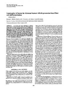
cell nuclei according to their differentiation code. This code corresponds to the founder cell of a lineage tree’s sublineages. While our 4 level condition used AB and P1 as the founder cells, the 6 and 7 level conditions used eight founder cells corresponding to the constituents of the 8-cell embryo (ABal, ABar, ABpl, ABpr, C, E, MS, and P3). These visualizations demonstrate separability between subtrees. To quantify and further investigate this spatial segregation, we use a k-means classification method and compare these categories with the differentiation code classification. To better understand the resulting overlap in categories, we use an intercalation analysis to find signatures of biological intercalation. While biological intercalation commonly occurs in mosaic development, it can often mimic our criterion of regulative development. Another phenomenon that can be confused with regulative development are ballistic cell migrations. To test for cell migrations, we use an exponential cell migration analysis to detect quasi-stochastic cell migrations that occur according to an exponential distribution. Finally, we use a connectivity measure to build an undirected network of relationships between cells. The structure of this network will provide information about interactions between cells. Comparisons between a random network (cells placed in random positions) and a C. elegans embryo network (Alicea, 2018) reveals that the network topologies presented here contain rich structural information. However, we do not make any claims about the significance of different connectivity regimes (see Albert 2005) other than to point out their relationship to geometric features of the embryo. Taken collectively, these analyses will allow us to distinguish between deterministically specified cell fates and cell fates that result from regulative influences. Visualization of Lineage Trees. The first analysis demonstrates that dividing the lineage tree into two sublineages reveals spatial segregation amongst cells in each subtree. The spatial locations of cells in these subtrees is shown in Figures 1A, 1B, and 1C. Figure 1A shows cells from the 4 level tree, Figure 1B from the 6 level tree, and Figure 1C from the 7 level tree. We can learn some basic relational lessons from this qualitative set of comparisons. The left panel of Figure 2 shows spatial separability along the left-right (L-R) axis, while the right panel of Figure 2 demonstrates spatial separability long the anterior-posterior (A-P) axis. While the spatial segregation of cells decreases with the birth of new cells, in the 7 level example (Figure 1C) there are clusters of cells that are descended exclusively from each subtree. Figure 2 shows the results of Figures 1A through 1C on the basis of comparing two major axes of variance (anterior-posterior and left-right) for the eight major subtrees in the lineage tree. Each major subtree descends from a single cell in the 8-cell embryo. For the two examples in Figure 2, variation along the anterior-posterior (A-P) dimension is compared to variation along the leftright (L-R) dimension for six of the eight subtrees in C. elegans the lineage tree. Data from the 6 level stage are shown. k-means Classification of Subtrees. A more quantitative way to measure the degree of spatial integration across development is to use biologically-based categories with the outcome of an unsupervised classification process. A k-means cluster analysis based on the x,y,z position of the cells is used to demonstrate this for trees rooted at both two founder cells (16-, 64-, and 128-cell condition) and eight founder cells (64- and 128-cell condition). As we can see in Table 1, the k6 PeerJ Preprints | https://doi.org/10.7287/peerj.preprints.26587v2 | CC BY 4.0 Open Access | rec: 19 Sep 2018, publ: 19 Sep 2018

means groups are highly predictive of lineage subtrees (G1 predicts AB at a rate of 0.8, and G2 predicts P1 at a rate of 0.8) in the 16 cell condition, but become less predictive as the tree grows in size. Even for the 128 cell condition, the k-means groups are moderately predictive (0.56 for G1 and 0.64 for G2).

Figure 1. A: Visualization of spatial segregation by differentiation code for the 16-cell condition (N = 30), embedded in a bounding box (black) that represents the extent of embryo space. B: Visualization of spatial segregation by differentiation code for the 64-cell condition (N = 114), embedded in a bounding box (black) that represents the extent of embryo space. C: Visualization of spatial segregation by differentiation code for the 128-cell condition (N = 224), embedded in a bounding box (black) that represents the extent of embryo space. In Tables 2 and 3, k-means generated groups are even less likely to predict the position of sublineages based on eight founder cells. There are, however, specific groups that are moderately predictive (0.4 to 0.7) of sublineage. For Table 2 (the 64 cell condition), these include group 4 as a predictor of cells in the C and P3 sublineages and group 8 as a predictor of the ABar sublineage. For Table 3 (the 128 cell condition), these include group 1 as a predictor of cells in the C sublineage and group 5 as a predictor of the ABal sublineage. 7 PeerJ Preprints | https://doi.org/10.7287/peerj.preprints.26587v2 | CC BY 4.0 Open Access | rec: 19 Sep 2018, publ: 19 Sep 2018

Table 1. Comparison of k-means cluster analysis (k=2) versus the AB and P1 subtrees for 16, 64, and 128 cell conditions. G1-G2 represents the groups generated by the k-means analysis, and the sublineage groups are identified by their lineage tree nomenclature. Each sublineage has a percentage of cells in each k-means generated group so that the sum of values across each row equal 1.00 (see Methods for more detail). 16 cell condition G1 G2 AB 0.80 0.20 P1 0.20 0.80 64 cell condition G1 G2 AB 0.67 0.33 P1 0.20 0.80 128 cell condition G1 G2 AB 0.56 0.44 P1 0.36 0.64 There were no obvious outliers in the input data for Tables 1-3, which resulted in minimal observed variation between simulation runs. It should be noted that the reported numbers for kmeans group membership will only vary slightly with multiple applications of the k-means algorithm (see Methods), embryos of a different species (e.g. less stereotypic than C. elegans), and different values of k. Intercalation Analysis. The intercalation analysis tests for uniform changes over time in spatial position amongst cell nuclei in a certain differentiation code subtree. Biological intercalation occurs by a set of cells (e.g. a tissue) narrowing along one anatomical axis while simultaneously expanding along an orthogonal axis. We test for this by making pairwise comparisons of correlation in variance for each differentiation code category along the A-P (x), L-R (y), and D-V (z) axes (Supplemental Table 1). This results in the following cross-correlations: x-y, y-z, and x-z. Table 2. Comparison of k-means cluster analysis (k=8) versus subtrees based on eight founder cells for 64-cell condition (114 node tree with 6 levels). G1-G8 represents the groups generated by the k-means analysis, and the sublineage groups are identified by their lineage tree nomenclature. Each sublineage has a percentage of cells in each k-means generated group so that the sum of values across each row equal 1.00 (see Methods for more detail). G1 G2 G3 G4 G5 G6 G7 G8 ABpl 0.00 0.13 0.27 0.00 0.00 0.13 0.27 0.20 ABpr 0.20 0.00 0.07 0.27 0.00 0.33 0.13 0.00 ABar 0.00 0.13 0.33 0.00 0.00 0.00 0.13 0.40 ABal 0.00 0.33 0.00 0.00 0.60 0.00 0.00 0.07 MS 0.00 0.13 0.4 0.07 0.00 0.13 0.2 0.07 E 0.00 0.00 0.13 0.33 0.00 0.27 0.27 0.00 C 0.27 0.00 0.00 0.53 0.00 0.07 0.13 0.00 8 PeerJ Preprints | https://doi.org/10.7287/peerj.preprints.26587v2 | CC BY 4.0 Open Access | rec: 19 Sep 2018, publ: 19 Sep 2018

P3

0.33

0.00

0.00

0.56

0.00

0.11

0.00

0.00

Figure 2. Anterior-posterior axis versus left-right axis variation for various octopartite subtrees for a 6 level tree (fixed axial plane). TOP: ABar (010), ABpl (000), ABpr (011). BOTTOM: ABal (011), MS (100), P3/P4/D (111). All identities: Lineage subtree (Differentiation subtree). For the 4 level condition, these cross-correlations were obtained for the two subtrees of the two founder cell lineage trees. This results in cells of the AB sublineage exhibiting a weak positive correlation amongst the x-y comparisons, but an anti-correlation for the y-z and x-z comparisons. For the 6 level condition, the cross-correlations were obtained for lineage subtrees based on eight founder cells. In the case of the x-y comparison, this results in moderately-tostrong negative correlations for the ABpl, ABpr, and ABal sublineages and no moderately-to9 PeerJ Preprints | https://doi.org/10.7287/peerj.preprints.26587v2 | CC BY 4.0 Open Access | rec: 19 Sep 2018, publ: 19 Sep 2018

weak positive correlations. For the y-z comparison, this results in moderately-to-strong negative correlations for the MS and E sublineages and moderately-to-weak positive correlations for the ABar sublineage. The x-z comparison, this results in no moderately-to-strong negative correlations but moderately-to-weak positive correlations for the E and P3 sublineages. These results mostly hold for the 7 level condition, despite the addition of data from another round of cell division. Table 3. Comparison of k-means cluster analysis versus each subtree for 128-cell condition (230 node tree with 7 levels). G1-G8 represents the groups generated by the k-means analysis, and the sublineage groups are identified by their lineage tree nomenclature. Each sublineage has a percentage of cells in each k-means generated group so that the sum of values across each row equal 1.00 (see Methods for more detail). G1 G2 G3 G4 G5 G6 G7 G8 ABpl 0 0.20 0.29 0.06 0.03 0.26 0 0.16 ABpr 0.23 0.03 0 0.32 0 0.07 0.35 0 ABar 0 0.32 0.07 0 0.03 0.26 0.13 0.19 ABal 0 0.13 0 0 0.52 0 0 0.35 MS 0 0.13 0.26 0.03 0 0.32 0.16 0.10 E 0.08 0 0.24 0.36 0 0.16 0.16 0 C 0.56 0 0 0.33 0 0 0.11 0 P3 0.24 0 0.18 0.35 0 0 0.23 0 Aggregate Cell Migration Analysis. To understand the role of diffusion in the early C. elegans embryo, we calculate the three-dimensional distance between all mother-daughter cell pairs at different stages (16-cell condition, 64-cell condition, and 128-cell condition) of early embryogenesis. Table 4 shows the results of this analysis. The distances between motherdaughter pairs are ranked according to distance. A power law exponent (α) is then calculated for the 4, 6, and 7 level conditions. Negative values of α greater than 1.0 represent a superdiffusive effect with movements after division from the mother cell at more than one distance scale. Superdiffusion translates into relatively rare instances of large scale displacements against a background of shorter displacements. The results in Table 4 show no trend towards a superdiffusive process in time as the embryo gains cells but a slight evidence for a superdiffusive process in space as one moves from the A-P axis to the L-R axis and then to the D-V axis. This result is consistent with the lineage tree being organized along the A-P axis, as it exhibits the most regularity in terms of positioning. While this matches a trend towards decreasing size along each of these axes, this analysis pulls out the rare large diffusion of a daughter cell along that axis. Table 4. Power law exponent (O) for 16-cell, 64-cell, and 128-cell embryos for each spatial axis. α 16-cell 64-cell 128-cell A-P axis 0.8 0.67 0.78 L-R axis 1.08 0.91 0.93 10 PeerJ Preprints | https://doi.org/10.7287/peerj.preprints.26587v2 | CC BY 4.0 Open Access | rec: 19 Sep 2018, publ: 19 Sep 2018

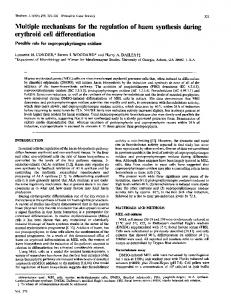
D-V axis 1.15 1.05 1.05 Network Analysis. The first analysis involved constructing a complex network out of a lineage tree by comparing the three-dimensional position of the nodes in a pairwise fashion. This comparison is done by calculating a Euclidean distance between each pair of cells, and then normalizing to the maximum value (see Methods). These comparisons were stratified by both Euclidean distance threshold and a distinction between subtrees AB and P1. The first analysis involves examining the potential interactions between cells at different distances in the lineage tree. For example, comparisons can be restricted to all cell pairs at the same level in the lineage tree, cells that are only one level away, cells two levels away, and cells that are 3-7 levels away. This provides a baseline for subsequent analyses which smear the time interval component of the lineage tree. Supplemental Figure 1 shows a series of circular graphs for network topologies for all potential interactions between pairs of cells at different levels of the lineage tree (calculated for cells at different differentiation tree depths). All networks are based on data from 7 level condition (N=224). Table 5 shows that there is diffusion across space as the subtrees grow in terms of depth based on an analysis of inter- and intra-subtree connections shown in Supplemental Figure 1. As several rounds of proliferation separate cell pairs in the same sublineage, they tend to spread out either axially or concentrically. This diffusion according to developmental time is best explained as a shift from intra-subtree to inter-subtree above-threshold connectivity as cellular relationships become separated over time (e.g. lineage tree depth). Table 5. Pairwise comparisons for a 7 level tree where embryo space distances were calculated for cells at different differentiation tree depths and both within and between sublineages. Values represent the percentage of interactions in each distance class for that category. The threshold for the distance metric was 0.75. Intra (AB) represents all pairwise comparisons where cells are descended from AB, Intra (P1) represents all pairwise comparisons where cells are descended from P1. Distance Intra- (AB, AB) Intra- (P1, P1) Inter – (AB, P1) between (i,j) comparisions only comparisons only comparisons only 0 57% 31% 12% 1 43% 35% 22% 2 27% 28% 45% 3-7 13% 13% 74% Table 5 reveals that for a fixed distance threshold (0.75), we can compare distances between cells across different linage tree levels to examine whether different sublineages remain mutually exclusive in their long-range interaction, or whether interactions between sublineages might be revealed across several cell divisions. In this case, we can see that lineage distance increases (e.g. distant ancestor vs. distant descendent), comparisons dominate the network at threshold 0.75. Figures 3, 4, and 5 show circular network topologies for the 16-, 64-, and 7 level conditions, respectively. Sublineages AB and P1 are color-coded: the nodes and intra-subtree connections for AB are shown in yellow, while the nodes and intra-subtree connections for P1 11 PeerJ Preprints | https://doi.org/10.7287/peerj.preprints.26587v2 | CC BY 4.0 Open Access | rec: 19 Sep 2018, publ: 19 Sep 2018

are shown in purple. Connections that span the subtrees are shown in gray, while an analysis of these network topologies are shown in Figure 5.

Figure 3. Circular layout of network topology with descendants of the smaller 2-cell division on the left and the larger 2-cell division on the right. Undirected complex network for all cells (represented as nodes) in 4 level condition (N = 30). Threshold is 0.75. Yellow and purple arcs are intra-sublineage connections (smaller and larger, respectively), while the light red arcs are inter-sublineage connections. Table 6 connects Figures 1A, 1B, and 1C to Figures 3, 4, and 5 by showing the network summary statistics for different distance thresholds for the 16-cell, 64-cell, and 128-cell embryos. As lineage trees get larger, the average degree tends to get larger for greater distances. The two most important results are that network modularity increases with relative distance, and that the number of communities increases dramatically as the relative distance threshold increases (and relative distance decreases). While these measures are interrelated, the community metric in particular provides strong evidence that dense patches of local connectivity becomes apparent at very limited spatial scales (5% of the entire embryo). To gain a better understanding of how geometric and spatial heterogeneity of the early embryo relate to cell lineage, we conducted two analyses related to connectivity. As connectivity 12 PeerJ Preprints | https://doi.org/10.7287/peerj.preprints.26587v2 | CC BY 4.0 Open Access | rec: 19 Sep 2018, publ: 19 Sep 2018

is defined as the potential interaction between cells within a given Euclidean distance, both analyses utilized data from the 128-cell condition at a threshold of 0.75 (25% of the maximum distance across the embryo). The results of these analyses are shown in Figures 3 (4 level), 4 (6 level), and 5 (7 level). These circular network plots demonstrate rich local and cross-connectivity between each subtree. Table 8 shows the proportion of connections between cells within and between each subtree in the two founder cell lineage tree for a given distance threshold.

Figure 4. Circular layout of network topology with descendants of the smaller 2-cell division on the left and the larger 2-cell division on the right. Undirected complex network for all cells (represented as nodes) in the 6 level condition (N = 114). Threshold is 0.95. Yellow and purple arcs are intra-sublineage connections (smaller and larger, respectively), while the light red arcs are inter-sublineage connections. From this analysis of connections based on Euclidean distance (Table 7), roughly 70-80% of all connections across early embryogenetic time are within a subtree. This is consistent with the 3-D spatial location plots shown in Figures 1A, 1B, and 1C. The only aberration in this pattern is in the 6 level embryo, where the number of intra-connections within the P1 subtree rise 13 PeerJ Preprints | https://doi.org/10.7287/peerj.preprints.26587v2 | CC BY 4.0 Open Access | rec: 19 Sep 2018, publ: 19 Sep 2018

to 46% at the expense of inter-subtree connections. The P1 subtree contains all non-AB sublineages, which give rise to a number of specialized fates.

Figure 5. Circular layout of network topology with descendants of the smaller 2-cell division on the left and the larger 2-cell division on the right. Undirected complex network for all cells (represented as nodes) in the 7 level condition (N = 224). Threshold is 0.95. Yellow and purple arcs are intra-sublineage connections (smaller and larger, respectively), while the light red arcs are inter-sublineage connections. Table 8 shows the results of a clique analysis for the eight founder cell linage tree. A clique analysis for cliques of size 5 yielded 117 unique cliques. A majority of the nodes amongst all of the cliques found came from just two eight founder cell sublineages (C and ABpr). Furthermore, 75.2% of all cliques generated exhibited overlap between each subtree (AB and P1). This suggests that there is strong inter-subtree connectivity and thus local structure in the midline of the embryo, in particular involving cells from the C and ABpr sublineages. 14 PeerJ Preprints | https://doi.org/10.7287/peerj.preprints.26587v2 | CC BY 4.0 Open Access | rec: 19 Sep 2018, publ: 19 Sep 2018

Table 6. Network summary statistics for different terminal cell sizes (16, 64, and 128) and thresholds (0.25 to 0.95). Missing values (-) reflect threshold values for which an analyzable graph could not be produced. Average Network Graph Modularity* Number of Clustering Degree Diameter Density Communities Coefficient 0.25 29.13 2 1.005 0 1 0.93 0.50 23.6 3 0.814 0 1 0.85 16 0.75 14.4 5 0.497 0.34 2 0.78 0.85 8.53 8 0.294 0.46 3 0.71 0.95 0.25 103.79 2 0.92 0 1 0.94 0.50 81.88 3 0.73 0 1 0.87 64 0.75 45.51 5 0.41 0.35 2 0.80 0.85 25.91 9 0.23 0.54 3 0.76 0.95 5.6 14 0.05 0.8 11 0.74 0.25 0.50 145.8 3 0.654 0.226 2 0.85 128 0.75 77.58 6 0.348 0.372 2 0.79 0.85 41.37 10 0.185 0.560 3 0.74 0.95 7.83 20 0.035 0.834 9 0.72 * resolution = 2.0. Table 7. Pattern of intra-subtree versus inter-subtree connectivity patterns for three sizes of embryo distance network. Subtrees are based on the descendent of the smaller (subtree 0) and larger (subtree 1) cells of the 2-cell embryo. Number of Terminal Cells 16 64 128 Distance Threshold

0.75

0.95

0.95

Proportion of Intra-subtree Connections (total)

0.68

0.79

0.74

Proportion of Inter-subtree Connections

0.32

0.21

0.26

Proportion of Intra-subtree Connections (AB)

0.31

0.34

0.39

Proportion of Intra-subtree Connections (P1)

0.37

0.46

0.35

Supplemental Figure 2 shows a heat map (Wikipedia, 2018a) that displays the frequency of nodes in each 8-cell subtree category for all 117 identified cliques of size 5. Cells from sublineages ABpr and C are the most heterogeneous, being included in cliques with cells from multiple sublineages. These two sublineages are represented in most of the 117 cliques and contain cells from a wide variety of other sublineages. One exception to this heterogeneous trend 15 PeerJ Preprints | https://doi.org/10.7287/peerj.preprints.26587v2 | CC BY 4.0 Open Access | rec: 19 Sep 2018, publ: 19 Sep 2018

is the sublineage ABal. Not only do cells from ABal form homogeneous cliques, ABal also contributes the fewest number of cells to the 117 identified cliques. Another way to assess connectivity is by conducting an analysis of degree distributions for interactions within the AB (intra AB) and P1 (intra P1) subtrees, and interactions between cells from the AB and P1 subtrees (inter AB-P1). Figure 6 shows the differences in these distributions. Overall, there is a difference between intra AB/inter AB-P1 and intra P1, namely that intra P1 exhibits a slightly larger tail representing more cells of a higher degree. Yet there is also a difference between intra AB and inter AB-P1 in that inter AB-P1 exhibits a greater number of cells with a smaller degree. These trends may reflects the geometry of the embryo, and suggest that the P1 sublineage is more spatially heterogeneous than the AB sublineage overall.

Figure 6. An analysis of connectivity in AB subtree (upper left), P1 subtree (upper right), and connections between the AB and P1 subtrees (bottom). Plots show degree distribution (degree) vs. complementary cumulative distribution function (CCDF). Stratifying the data by lineage tree depth also suggests that certain sets of closely-related cells (and thus specific locations in the embryo) are the source of most of this nonlinearity. Figure 7 demonstrates this by visualizing the rank-order relationships in each of the levels (7) in a 7 level lineage tree. Consistently, the descendant cells of MS and ABpr serve as leastconnected outliers at their respective level. These cells represent 16 of the 17 labeled cells in Figure 7. Discussion and Broader Implications In this paper, we have introduced a method called embryo networks that can characterize the emergent properties of early embryogenesis. This approach not only explicitly represents the spatiotemporal complexity of the embryogenetic process, but also demonstrates that the 16 PeerJ Preprints | https://doi.org/10.7287/peerj.preprints.26587v2 | CC BY 4.0 Open Access | rec: 19 Sep 2018, publ: 19 Sep 2018

embryogenetic process operates on a variety of different temporal and spatial scales. Our work is motivated by the transformation of a symmetric structure to an asymmetric structure. Yet we can see that there is much more complexity than revealed by conceptual models of processes such as symmetry-breaking or pairwise branching. This study fills a gap in the literature by presenting a quantitative interpretation of the parallel and top-down processes inherent in embryogenesis.

Figure 7. A rank-order analysis of 128-cell condition (N = 224), stratified by lineage depth (ranging from 3-7). Outlier cells are labeled for each series. Moreover, we have introduced an approach to characterize the spatial emergence of structure at the cellular level during the embryogenetic process. It is an approach that encompasses network science, statistical analysis, and data visualization. Based on the averaged locations of founder cells as well as their subsequent daughter cells, we infer a network that provides a model of connectivity separate from but not independent of lineage relationships. While we utilize data from the nematode C. elegans to illustrate the concept, this approach to embryogenetic emergence has the potential to be broadly applicable to species across the tree of life. In terms of biological relevance, a network approach allows us to characterize the dynamic topology of the embryo's cell interactome in a quantitative fashion. This allows us to characterize potential signaling relationships between cells and over time as cells divide and their descendants acquire new spatial relationships. By taking into account the diffusion of cells upon division, we can also get a sense of how the global network topology shifts as the position of and interactions between adult cells are established. Our use of the differentiation code (Gordon, 1999) provides means to categorize cells by the lineage subtree based on size asymmetries amongst daughter cells (Alicea and Gordon, 2016). This allows us to classify the lineage tree in an alternate way that is more sensitive to phenotypic variation within developmental sublineages. 17 PeerJ Preprints | https://doi.org/10.7287/peerj.preprints.26587v2 | CC BY 4.0 Open Access | rec: 19 Sep 2018, publ: 19 Sep 2018

In a broader context, this may allow us to find potential modules or communities (Newman, 2006) in the network that equate to the differentiation of distinct tissue types. As lineage and differentiation trees become available for regulating embryos, the methods developed here may better allow us to understand the differences and similarities between mosaic and regulating embryos, postulated as being based in single cell versus multiple cell differentiation waves, respectively (Gordon, 1999; Gordon and Gordon, 2016). Table 8. Clique analysis for a 7 level network topology. Sublineage

Number of members of sublineage across all cliques generated

ABpl

ABpr

ABar

ABal

MS

E

C

P3

42

151

68

34

35

58

159

38

AB Number of cliques with overlap Number of cliques without overlap

P1 75.2%

15.4%

9.4%

By combining our approach to generativity, diffusion, and differentiation processes, we can also characterize a new phenomenon related to spatial segregation. As in cognitive brain networks, another advantage to a dynamic network approach is the potential to discover so-called temporal metastates (Shine et al., 2016). As a set of candidate measures and generalized methodology, a complex network model allows us to observe global relationships between embryo geometry, spatial distributions of cell lineages over time, and potential multivariate structural relationships. It should be noted that a similar method called the scale-invariant power law approach (Tiraihi et al., 2011) has been used to study self-organization in developing embryos. As the scale-invarient approach focuses on the entirely of the early embryo, it also treats macroscopic cellular proliferation as a scale-invariant process. In this study, approximations of cell positions and distances were used to estimate the geometry of the early embryo, with greater statistical variation expressed in the non-AB sublineages. This is similar to our results, as the non-AB lineages are quantitatively different from AB sublineages. Shortcomings and Future Work There are several unanswered questions regarding the relevance and outcomes of the embryo network approach, in addition to avenues for future work. The first issue is what structural and functional features the embryo network method actually represents. While it is hypothesized that the connections of our network represent juxtacrine and other types of proximity signaling, the network structure itself is indicative of the emergence of embryo geometry. This is not limited to C. elegans: networks created using cell centroid data from mouse 18 PeerJ Preprints | https://doi.org/10.7287/peerj.preprints.26587v2 | CC BY 4.0 Open Access | rec: 19 Sep 2018, publ: 19 Sep 2018

embryos (Strnad et al., 2016) demonstrate clear spatial segregation between the inner cell mass and trophectoderm (Alicea, 2018). Whether embryo networks reflect information about the combined effects of local signaling and the phenotypic geometry is not clear at this point. Future work might focus on discovering connections between network structure and topological models of embryology (Thom, 1972). The second issue involves how current methods of network analysis and visualization limit our ability to see these distinctions clearly. Network science has been colloquially called "hairball science" (Rottjers and Faust, 2018), which arises from the resemblance of even moderately-sized networks to hairballs that have no clear inputs and outputs nor causality. Plotting networks that emphasize one set of relationships often comes at the expense of another. For example, the circular plots shown in this paper do not clearly reveal spatial patterns, but do reveal global patterns of connectivity. Yet even here, it is hard to discern what these patterns actually mean in an anatomical context. Future work should involve rendering anatomically explicit and multilayer (Kivela et al., 2014) network topologies, such as the 4D tree sketched out for an ascidian (Figure 11.8 in Gordon and Gordon, 2016). A third issue is the true nature of networks based on developmental phenotypes. While our ability to find structure in the form of communities and weak connectors may be informative, the typical means of classifying global network properties may not be. While the technical distinctions between random, scale-free, and small-world global network topologies can be adapted to biological contexts (Prettejohn et al., 2011), the phenotypic and developmental informativeness of these categories may not be sufficient. At times, the meaning of concepts such as modularity intersect and serve to describe structural phenomena. Yet we need a different form of visualization and a new vocabulary to think about developmental phenotypes in terms of degree distributions. Conclusions How does this type of network analysis specifically inform us about the developmental process? Taken together with the k-means analysis, we can see that cells in Caenorhabditis elegans embryos only partially segregate by lineage and sublineage. Cells that are colocated, or in this case are directly connected with cells of a different sublineage, may serve as so-called weak connectors (Albert and Barabasi, 2002; Granovetter, 1983) in a network representation. In embryo networks, weak connectors can be defined as the connection between cells based solely on proximity rather than a combination of proximity and lineage identity. In this case, weak connectors serve to indirectly link different populations of cells in a way that would not be possible in a regulative developmental system. In a regulative embryo, a cell from one sublineage in close proximity to cells of another sublineage would acquire the fate of neighboring cells, if it is in the “competent”, but not yet “determined” state (Gordon, 1999). By capturing their position in the middle of the embryogenetic process, we can see how a given sublineage can be founded in a single spatial location and later spread out across the nematode body, performing either specialized or diverse functions. Discovering the identity of weak connectors is just one advantage of using this type of analysis in Caenorhabditis elegans: we can keep track of the ultimate fate of a given cell based 19 PeerJ Preprints | https://doi.org/10.7287/peerj.preprints.26587v2 | CC BY 4.0 Open Access | rec: 19 Sep 2018, publ: 19 Sep 2018

on its lineage identity. Therefore, no matter its temporary developmental position, we can make the distinction between a deterministic (analogous to mosaic development) and a semi-stochastic (analogous to regulative development) process. Future work might focus on extending these methods to regulative embryos using cellular barcoding techniques to infer developmental lineages (Perie et al., 2014). The final point stems from an intriguing outcome, suggested from the clique analysis, that specific sublineage groups can coexist in a spatial region of limited size. For example, some cliques might contain several closely-related cells (based on their position in the lineage tree), and a few cells that are from a separate sublineage. However, if the mosaic mode of development dominates, we should expect these interloping cells to remain autonomous and be defined by their lineage tree location rather than by their spatial position (e.g. the cells they interact with). Whether this has significant consequence for future differentiation is an open question that can be addressed by applying these techniques to other species and developmental contexts. As some regulation, i.e., differentiation dependent in part on cell-cell interactions, has been found in nematodes (Wiegner and Schierenberg, 1999), the next step in network analysis could be to find criteria for when cell-cell proximity has no effect or alters the fate of the cells. Acknowledgements We would like to acknowledge Drs. Zhirong Zhao and Stephen Larson for providing data on the C. elegans embryo. Thanks also go to members of the OpenWorm Foundation and the Network Science community for scientific feedback. Supplemental Files Supplemental File 1: circular network topologies comparing connections among subtrees and tree levels. The x-axis features a series of circular networks based on the number of above threshold connections between cells at different levels of the tree in a 7 level (128-cell condition) tree. Rows in descending order: no difference in tree level (0), difference of one level (1), difference of two levels (2), difference of between 3 and 7 levels (3-7). Columns from left to right: all connections between cells in the AB sublineage only (intra-AB), all connections between cells in the P1 sublineage only (intra-P1), all connections between cells where one cell is from the AB sublineage and the other cell is from the P1 sublineage (inter-AB-P1). Supplemental File 2: Heat map of the clique analysis for a 7 level (128-cell condition) tree. Each row represents a unique clique generated from a connectivity matrix of the 7 level tree. The heat map columns represent the number of members in the generated cliques from each subtree based on eight founder cells (8 categories). Color coding scheme is presented in the legend to the right of the map. Supplemental Table 1: Correlations of positional variance between three pairs of spatial dimensions (X-Y, Y-Z, and X-Z) and within differentiation code categories (4, 6, and 7 level). References Albert R. 2005. Scale-free networks in cell biology. Journal of Cell Science, 118, 4947-4957. doi: 10.1242/jcs.02714.

20 PeerJ Preprints | https://doi.org/10.7287/peerj.preprints.26587v2 | CC BY 4.0 Open Access | rec: 19 Sep 2018, publ: 19 Sep 2018

Albert R, Barabasi A-L. 2002. Statistical mechanics of complex networks. Reviews in Modern Physics, 74, 47. doi:10.1103/RevModPhys.74.47. Alicea, B. 2018. Process as Connectivity: models of interaction in cellular systems. Presented to "Finding Your Inner Modeler II" workshop, University of Illinois-Chicago, August 17. Figshare, doi:10.6084/m9.figshare.6983042. Alicea B, Gordon R. 2016. Quantifying Mosaic Development: Towards an Evo-Devo Postmodern Synthesis of the Evolution of Development Via Differentiation Trees of Embryos. Biology, 5(3), 33. doi:10.3390/biology5030033 Alicea B, McGrew S, Gordon R, Larson S, Warrington T, Watts M. 2014. DevoWorm: differentiation waves and computation in C. elegans embryogenesis. bioRxiv, doi:10.1101/ 009993. Arthur D, Vassilvitskii S. 2007. K-means++: the advantages of careful seeding. Proceedings of the ACM-SIAM Symposium on Discrete Algorithms (SODA), 1027–1035. Arthur W. 2011. Evolutionary Developmental Biology: Developmental Bias and Constraint. eLS: Citable Reviews in the Life Sciences, doi:10.1002/9780470015902.a0001066.pub3. Arthur D, Vassilvitskii S. 2007. K-means++: the advantages of careful seeding. Proceedings of the ACM-SIAM Symposium on Discrete Algorithms (SODA), 1027–1035. Bao ZR, Zhao ZY, Boyle TJ, Murray JI, Waterston RH. 2008. Control of cell cycle timing during C. elegans embryogenesis. Developmental Biology, 318(1), 65–72. doi:10.1016/j.ydbio.2008.02.054 Bao ZR, Murray JI, Boyle T, Ooi SL, Sandel MJ, Waterston RH. 2006. Automated cell lineage tracing in Caenorhabditis elegans. PNAS,103(8), 2707-2712. doi:10.1073/pnas.0511111103. Bao ZR, Zhao ZY, Boyle TJ, Murray JI, Waterston RH. 2008. Control of cell cycle timing during C. elegans embryogenesis. Developmental Biology, 318(1), 65–72. doi:10.1016/j.ydbio.2008.02.054 Blondel VD, Guillaume J, Lefebvre E. 2008. Fast unfolding of communities in large networks. Journal of Statistical Mechanics: Theory and Experiment, P10008. doi:10.1088/17425468/2008/10/P10008 Bolker JA. 2000. Modularity in Development and Why It Matters to Evo-Devo. Integrative and Comparative Biology, 40(5), 770–776. doi:10.1093/icb/40.5.770. Briscoe J, Small S. 2015. Morphogen rules: design principles of gradient-mediated embryo patterning. Development, 142, 3996-4009. doi: 10.1242/dev.129452.

21 PeerJ Preprints | https://doi.org/10.7287/peerj.preprints.26587v2 | CC BY 4.0 Open Access | rec: 19 Sep 2018, publ: 19 Sep 2018

Chen Q, Shi J, Tao Y, Zernicka-Goetz M. 2018. Tracing the origin of heterogeneity and symmetry breaking in the early mammalian embryo. Nature Communications, 9, 1819.doi:10.1038/s41467-018-04155-2. Dannemann T, Boyer D, and Miramontes O. 2018. Lévy flight movements prevent extinctions and maximize population abundances in fragile Lotka–Volterra systems. PNAS, 115(15), 37943799. doi.org/10.1073/pnas.1719889115. Dieterich P, Klages R, Preuss R, Schwab A. 2008. Anomalous dynamics of cell migration. PNAS, 105(2) 459-463. doi:10.1073/pnas.0707603105 Esteve-Altava B, Diogo R, Smith C, Boughner JC, Rasskin-Gutman, D. 2015a. Anatomical networks reveal the musculoskeletal modularity of the human head. Scientific Reports, 5, 8298. doi:10.1038/srep08298 Esteve-Altava B, Boughner JC, Diogo R, Villmoare BA, Rasskin-Gutman D. 2015b. Anatomical Network Analysis shows decoupling of modular lability and complexity in the evolution of the primate skull. PLoS One, 10(5), e0127653. doi:10.1371/journal.pone.0127653 Fagotto F. 2014. The cellular basis of tissue separation. Development, 141(17), 3303-3318. doi:10.1242/dev.090332 Fedotov S, Tan A, Zubarev A. 2015. Persistent random walk of cells involving anomalous effects and random death. Physical Review E, 91(4), 042124. doi:10.1103/PhysRevE.91.042124 Gordon R. 1999. The Hierarchical Genome and Differentiation Waves: Novel Unification of Development, Genetics and Evolution. Singapore & London, World Scientific & Imperial College Press. Gordon, R., Brodland, G.W., 1987. The cytoskeletal mechanics of brain morphogenesis. Cell state splitters cause primary neural induction. Cell Biophysics, 11(1), 177-238. doi:10.1007/BF02797122. Gordon NK, Gordon R. 2016. Embryogenesis Explained. Singapore, World Scientific Publishing Company. Granovetter M. 1983. The Strength of Weak Ties: A Network Theory Revisited. Sociological Theory, 1, 201–233. doi:10.2307/202051. Green RA, Kao HL, Audhya A, Arur S, Mayers JR, Fridolfsson HN, Schulman M, Schloissnig S, Niessen S, Laband K, Wang S, Starr DA, Hyman AA, Schedl T, Desai A, Piano F, Gunsalus KC, Oegema K. 2011. A high-resolution C. elegans essential gene network based on phenotypic profiling of a complex tissue. Cell, 145, 470-482. doi:10.1016/j.cell.2011.03.037 Gunsalus KC, Rhrissorrakrai K. 2011. Networks in Caenorhabditis elegans. Current Opinion in Genetics & Development, 21, 787–798. doi:10.1016/j.gde.2011.10.003

22 PeerJ Preprints | https://doi.org/10.7287/peerj.preprints.26587v2 | CC BY 4.0 Open Access | rec: 19 Sep 2018, publ: 19 Sep 2018

Gunsalus KC, Ge H, Schetter AJ, Goldberg DS, Han JD, Hao T, Berriz GF, Bertin N, Huang J, Chuang LS, Li N, Mani R, Hyman AA, Sonnichsen B, Echeverri CJ, Roth FP, Vidal M, and Piano F. 2005. Predictive models of molecular machines involved in Caenorhabditis elegans early embryogenesis. Nature, 436, 861-865. doi:10.1038/nature03876. Guo J, Lin F, Zhang X, Tanavde V, Zheng J. 2017. NetLand: quantitative modeling and visualization of Waddington's epigenetic landscape using probabilistic potential. Bioinformatics, 33(10), 1583-1585. doi: 10.1093/bioinformatics/btx022. Kivela M, Arenas A, Barthelemy M, Gleeson JP, Moreno Y, Porter MA. 2014. Multilayer networks. Journal of Complex Networks, 2(3), 203–271. doi:10.1093/comnet/cnu016. Lokeshwar BL, Nanjundiah V. 1980/1981. The scale-invariance of spatial patterning in a developing system. Wilhelm Roux's Archives of Developmental Biology, 190(6), 361-364. Murray JI, Boyle TJ, Preston E, Vafeados D, Mericle B, Weisdepp P, Zhao Z, Bao Z, Boeck M, Waterston RH. 2012. Multidimensional regulation of gene expression in the C. elegans embryo. Genome Research, 22(7), 1282-1294. doi:10.1101/gr.131920.111 Newman MEJ. 2006. Modularity and community structure in networks. PNAS, 103(23), 85778582. doi:10.1073/pnas.0601602103 Newman MEJ. 2003. The Structure and Function of Complex Networks. SIAM Review, 45(2), 167–256. doi:10.1137/S003614450342480 Nishida H, Stach T. 2014. Cell lineages and fate maps in tunicates: conservation and modification. Zoological Science, 31(10), 645-652. doi:10.2108/zs140117 Perie L, Hodgkin PD, Naik SH, Schumacher TN, de Boer RJ, Duffy KR. 2014. Determining Lineage Pathways from Cellular Barcoding Experiments. Cell Reports, 6(4), 27, 617-624. doi:10.1016/j.celrep.2014.01.016. Prettejohn BJ, Berryman MJ, and McDonnell, MD. 2011. Methods for Generating Complex Networks with Selected Structural Properties for Simulations: A Review and Tutorial for Neuroscientists. Frontiers in Computational Neuroscience, 5, 11. doi:10.3389/fncom.2011.00011. Rottjers L, Faust K. 2018. From hairballs to hypotheses: biological insights from microbial networks. FEMS Microbiology Review, doi:10.1093/femsre/fuy030. Schnabel R, Bischoff M, Hintze A, Schulz AK, Hejnol A, Meinhard H, Hutter H, 2006. Global cell sorting in the C. elegans embryo defines a new mechanism for pattern formation. Developmental Biology, 294(2), 418-431. doi:10.1016/j.ydbio.2006.03.004 Schnabel R. 1996. Pattern formation: regional specification in the early C. elegans embryo. Bioessays, 18(7), 591-594. doi:10.1002/bies.950180711

23 PeerJ Preprints | https://doi.org/10.7287/peerj.preprints.26587v2 | CC BY 4.0 Open Access | rec: 19 Sep 2018, publ: 19 Sep 2018

Shine JM, Koyejo O, Poldrack RA. 2016. Temporal metastates are associated with differential patterns of time-resolved connectivity, network topology, and attention. PNAS, 113(35), 98889891. https://doi.org/10.1073/pnas.1604898113. Sonnichsen B, Koski L, Walsh A, Marshall P, Neumann F, Brehm M, Alleaume A-M, Bettencourt P, Cassin E, Hewitson M, Holz C, Khan M, Lazik S, Martin C, Nitzsche B, Ruer M, Stamford J, Winzi M, Heinkel R, Roder M, Finell J, Hantsch H, Jones SJM, Jones M, Piano F, Gunsalus KC, Oegema K, Gonczy P, Coulson A, Hyman AA, Echeverri CJ. 2005. Full-genome RNAi profiling of early embryogenesis in Caenorhabditis elegans. Nature, 434, 462-469. doi:10.1038/nature03353. Stadler T, Skylaki S, Kokkaliaris KD, Schroeder T. 2018. On the statistical analysis of single cell lineage trees. Journal of Theoretical Biology, 439, 160-165. Stone R, Portegys T, Mikhailovsky G, Alicea B. 2018. Origins of the Embryo: self-organization through cybernetic regulation. BioSystems, doi:10.1016/j.biosystems.2018.08.005. Stone R, Gordon R. 2017. Cybernetic embryo. In “Biocommunication” R. Gordon and J. Seckbach eds., pgs. 111-164. London: World Scientific Publishing. doi:10.1142/9781786340450_0005. Strnad P, Gunther S, Reichmann J, Krzic U, Balazs B, de Medeiros G, Norlin N, Hiiragi T, Hufnagel L, Ellenberg J. 2016. Inverted light-sheet microscope for imaging mouse preimplantation development. Nature Methods, 13(2), 139-142. doi: 10.1038/nmeth.3690. Sulston JE, Schierenberg E, White JG, Thomson, JN. 1983. The embryonic cell lineage of the nematode Caenorhabditis elegans. Developmental Biology, 100(1), 64-119. Thom R. 1972. Structural Stability and Morphogenesis: an outline of a general theory of models. W.A. Benjamin, New York. Tiraihi A, Tiraihi M, Tiraihi T. 2011. Self-organization of developing embryo using scaleinvariant approach. Theoretical Biology and Medical Modelling, 8, 17. doi:10.1186/1742-46828-17 Walck-Shannon E, Hardin J. 2014. Cell intercalation from top to bottom. Nature Reviews Molecular Cell Biology, 15, 34-48. doi:10.1038/nrm3723 Wetts R, Fraser SE. 1989. Slow intermixing of cells during Xenopus embryogenesis contributes to the consistency of the blastomere fate map. Development, 105(1), 9-15. Wiegner, O., Schierenberg, E., 1999. Regulative development in a nematode embryo: A hierarchy of cell fate transformations. Developmental Biology, 215(1), 1-12. Wikipedia, 2018a. Heat map. https://en.wikipedia.org/wiki/Heat_map Wikipedia, 2018b. Interactome. https://en.wikipedia.org/wiki/Interactome 24 PeerJ Preprints | https://doi.org/10.7287/peerj.preprints.26587v2 | CC BY 4.0 Open Access | rec: 19 Sep 2018, publ: 19 Sep 2018

Woods ML, Carmona-Fontaine C, Barnes CP, Couzin ID, Mayor R, Page KM. 2014. Directional Collective Cell Migration Emerges as a Property of Cell Interactions. PLoS One, 9(9), e104969. doi:10.1371/journal.pone.0104969. Zhang HT, Hiiragi T. 2018. Symmetry Breaking in the Mammalian Embryo. Annual Review of Cell and Developmental Biology, 34. doi:10.1146/annurev-cellbio-100617-062616.

25 PeerJ Preprints | https://doi.org/10.7287/peerj.preprints.26587v2 | CC BY 4.0 Open Access | rec: 19 Sep 2018, publ: 19 Sep 2018