PHYSICAL REVIEW E 76, 026105 共2007兲
Cellular-automaton model with velocity adaptation in the framework of Kerner’s three-phase traffic theory 1
Kun Gao,1,* Rui Jiang,2,† Shou-Xin Hu,3 Bing-Hong Wang,1,‡ and Qing-Song Wu2
Nonlinear Science Center and Department of Modern Physics, University of Science and Technology of China, Hefei, Anhui, 230026, People’s Republic of China 2 School of Engineering Science, University of Science and Technology of China, Hefei, Anhui, 230026, People’s Republic of China 3 Department of Science, Bengbu College, Bengbu, Anhui, 233050, People’s Republic of China 共Received 8 February 2007; revised manuscript received 5 June 2007; published 13 August 2007兲 In this paper, we propose a cellular automata 共CA兲 model for traffic flow in the framework of Kerner’s three-phase traffic theory. We mainly consider the velocity-difference effect on the randomization of vehicles. The presented model is equivalent to a combination of two CA models, i.e., the Kerner-Klenov-Wolf 共KKW兲 CA model and the Nagel-Schreckenberg 共NS兲 CA model with slow-to-start effect. With a given probability, vehicle dynamical rules are changed over time randomly between the rules of the NS model and the rules of the KKW model. Due to the rules of the KKW model, the speed adaptation effect of three-phase traffic theory is automatically taken into account and our model can show synchronized flow. Due to the rules of the NS model, our model can show wide moving jams. The effect of “switching⬙ from the rules of the KKW model to the rules of the NS model provides equivalent effects to the “acceleration noise⬙ in the KKW model. Numerical simulations are performed for both periodic and open boundaries conditions. The results are consistent with the well-known results of the three-phase traffic theory published before. DOI: 10.1103/PhysRevE.76.026105
PACS number共s兲: 89.40.⫺a, 45.70.Vn, 05.40.⫺a, 02.60.Cb
I. INTRODUCTION
Traffic flow phenomena have attracted the interest of physicists since the early 1990s. Many models and analysis are carried out from the viewpoint of statistical physics by various groups recent years, in order to explain the empirical findings 关1–12兴. Among them, cellular automata 共CA兲 models, as an important category, have become a well-established method to model, analyze, understand, and even forecast the behaviors of real road traffic since Nagel and Schreckenberg proposed a “minimal⬙ CA model in 1992 which has become the basic model of this field and is called the NagelShreckenberg 共NS兲 model 关13兴. So far, most of these traffic models are due to the socalled “fundamental diagram approach,” in which the steady state solutions belong to a curve in the flow-density plane 关14–18兴. Correspondingly, this curve going through the origin with at least one maximum is called “the fundamental diagram” for traffic flow. The fundamental diagram approach is successful in explaining several aspects of real traffic, such as the forming of queue, the dissolution of jams, etc. The congested patterns from the fundamental diagram approach are due to the instability of steady states of the fundamental diagram within some range of vehicle densities. When perturbed, a transition from metastable free flow to jam 共F → J兲 occurs and the traffic decays into a single or a sequence of wide moving jams. Nevertheless, a more detailed analysis of empirical data has been given by Kerner recently 关8–12兴. Based on these empirical data, it was found out that in congested traffic two
*
[email protected] †
[email protected] [email protected]
‡
1539-3755/2007/76共2兲/026105共7兲
different traffic phases should be distinguished: “synchronized flow” and “wide moving jams.” Therefore, there are three traffic phases: 共1兲 free flow, 共2兲 synchronized flow, 共3兲 wide moving jams. Wide moving jams do not emerge spontaneously in free flow. Instead, there is a sequence of two first order phase transitions: first the transition from free flow to synchronized flow occurs 共F → S兲, and later and usually at a different location moving jams emerge in the synchronized flow 共S → J兲. It is also pointed out by Kerner that the dynamical behavior near an on-ramp differs significantly in the fundamental diagram approach and in empirical observations. For example, in the diagram of congested states based on the fundamental diagram approach, at the highest values of on-ramp flow rate, the homogeneous congested traffic 共HCT兲 occurs and no jam appears 关15–18兴. This is in contradiction with empirical observations where wide moving jams always emerge spontaneously in general pattern 共GP兲 关4兴. Moreover, at the low values of on-ramp flow rate, jams always emerge as a single moving local cluster 共MLC兲 or triggered stopand-go traffic 共TSG兲 in the fundamental diagram approach 关15–18兴. However, synchronized patterns 共SP兲 with high speed and flow rate that is as great as in free flow appear in empirical observations in which no wide moving jams occur 关4兴. Based on empirical observations, Kerner developed a three-phase traffic theory 关19–24兴. The fundamental hypothesis of this theory is that the steady states of synchronized flow cover a two-dimensional 共2D兲 region in the flowdensity plane 关25,26兴. That is to say, a fundamental diagram of traffic flow in this theory does not exist. In a traffic model based on this theory, moving jams do not spontaneously occur in free flow. Instead, the first-order phase transition to synchronized flow beginning at some density in free flow is realized. The moving jams emerge only in synchronized
026105-1
©2007 The American Physical Society
PHYSICAL REVIEW E 76, 026105 共2007兲
GAO et al.
flow. As a result, the diagrams of traffic patterns both for a homogeneous road without bottlenecks and at on-ramps are qualitatively different from those found in the fundamental diagram approach. Kerner believes that a model within the framework of three-phase traffic theory should be able to 共at least qualitatively兲 reproduce the empirical observed spatiotemporal patterns. In 2002, Kerner and Klenov developed a microscopic model of the three-phase traffic theory, which can reproduce empirical spatiotemporal patterns 关27兴. Later, microscopic models based on three phase traffic theory have been developed, such as the Kerner-Klenov-Wolf 共KKW兲 CA model 关19,28兴, the CA model introduced by Lee et al. 关29兴, which considers the mechanical restriction versus human overreaction, the model proposed by Davis 关30兴, the model of Jiang and Wu 关31,32兴, and the deterministic models proposed by Kerner and Klenov 关33兴. As in empirical observations, these models exhibit the sequence of F → S → J transitions leading to wide moving jams emergence beginning from free flow. In addition, the models show all types of congested patterns found in empirical observations. In this paper, we are going to propose another CA model on the basis of the existing models in the framework of three-phase traffic theory. We mainly consider the velocitydifference effect on the randomization of vehicles in this model. It will be shown later that the presented model is equivalent to a combination of two CA models, i.e., the KKW model 关19,28兴 and the NS model with slow-to-start effect 关34兴. This model can show both synchronized flow and wide moving jams, which will be exhibited in the latter part of this paper. The rest of this paper is organized as follows. In Sec. II, we describe our model. In Sec. III, simulations on roads under both periodic and open boundary conditions are presented. In Sec. IV, we conclude. II. THE MODEL
In this section we present our model. The main mechanisms associated with three-phase traffic theory in this model are embodied in the randomization process of vehicles. The parallel update rules are as follows. 共1兲 Determining the randomization probability pn共t + 1兲 and the deceleration extent ⌬v. pn共t + 1兲 =
⌬v =
冦冦
再
p0 when tst,n 艌 tc , pd when tst,n ⬍ tc ,
a b− if 关vn共t兲 ⬍ vn−1共t兲兴 b0 if 关vn共t兲 = vn−1共t兲兴 b+ if 关vn共t兲 ⬎ vn−1共t兲兴
冧
冎
when tst,n 艌 tc when tst,n ⬍ tc .
共1兲
冧
vn共t + 1兲 = min关vn共t + 1兲,dn兴.
共4兲 Randomization with probability pn共t + 1兲: vn共t + 1兲 = max关vn共t + 1兲 − ⌬v,0兴.
共5兲 The determination of tst,n: tst,n =
再
tst,n + 1
if 关vn共t + 1兲 = 0兴
0
if 关vn共t + 1兲 ⬎ 0兴.
共3兲
共6兲 Vehicle motion: xn共t + 1兲 = xn共t兲 + vn共t + 1兲. Here xn共t兲 and vn共t兲 are the position and velocity of vehicle n at time t 共here vehicle n − 1 precedes vehicle n兲, dn is the gap of vehicle n, i.e., the distance from the head of vehicle n to the tail of vehicle n − 1, tst,n denotes the time that vehicle n stops, and tc is a slow-to-start parameter. The following rank of the acceleration and deceleration parameters are required: b+ 艌 a 艌 b− .
共4兲
In the rules above, Eqs. 共1兲 and 共3兲 represent the slow-tostart effect. Following the work of Jiang and Wu, it is fulfilled by considering the stop times of vehicles. In our viewpoint, the driver’s attention will be kept concentrated when encountering short-time halt in traffic, but distracted after a long time waiting. 共For example, someone may read a newspaper or even go out of the car. This is simulated by large randomization.兲 So the slow-to-start would happen only with a long stop time. The threshold parameter tc is set for this. We will discuss on the effect of tc later. On the other hand, Eqs. 共2兲 and 共4兲 describe the speed adaptation effect. When the velocity is larger than the velocity of the leading vehicle, the driver will tend to overreact when decelerating. The deceleration extent will be relatively large, corresponding to the largest parameter b+. In order to simulate the synchronized flow, Eq. 共4兲 is sufficient and necessary. As a result, when randomization occurs, the vehicle will adjust its velocity close to the velocity of the leading vehicle. This is consistent with the basic rules of the KKW model 关19,28兴. Actually, the presented model is equivalent to a combination of two existing CA models, i.e., the KKW model and the NS model with slow-to-start effect. To show this, we consider our model in the intermediate range of vehicle speed, which are the most interesting for simulations of synchronized flow. When vn共t兲 + a 艋 vmax, vn共t兲 + a 艋 dn, and tst,n ⬍ tc, namely, there are no restrictions related to the maximum speed vmax and the safe speed dn, respectively, and also no slow-to-start rule, the updating rule of our model is
冦
a − b− 艌 0 if 关vn共t兲 ⬍ vn−1共t兲兴, if 关vn共t兲 = vn−1共t兲兴, vn共t + 1兲 = vn共t兲 + a − b0 a − b+ 艋 0 if 关vn共t兲 ⬎ vn−1共t兲兴
共2兲
共2兲 Accelerating: vn共t + 1兲 = min关vn共t兲 + a, vmax兴.
共3兲 Braking:
冎
with probability pd or 026105-2
冧
共5兲
PHYSICAL REVIEW E 76, 026105 共2007兲
CELLULAR-AUTOMATON MODEL WITH VELOCITY…
FIG. 1. 共Color online兲 The two-dimensional region of the equilibrium states of synchronized flow in a noiseless limit, in which pd → 1. Assuming the length of a single vehicle is 7.5 m and the maximum velocity is 37.5 m / s.
are all embodied in the randomization process, the noiseless limit is taken as pd → 1 rather than pd → 0. In this case, the updating rules of the KKW model are adopted. As shown in Refs. 关19,27兴, the two-dimensional region of the equilibrium states is restricted by three boundaries in the flow-density plane: the upper 共line U兲, the lower 共line L兲, and the left 共line F兲 boundaries. Compared to the basic rule of the KKW model, the only difference in the rules of our model is that there does not exist such a parameter as the synchronization distance D共v兲, which describes the maximal distance at which the vehicle takes into account the speed of the leading vehicle when accelerating 关19,27兴. In other words, our model can be regarded as a limit of the KKW model when D共v兲 → ⬁. As a result, the lower boundary L of the twodimensional region approaches the x axis. As in the KKW model, the upper boundary U is determined by the safe speed of vehicles, which is determined by the headway distance 共in equilibrium states, we assume all the vehicles have a uniform speed and headway distance兲. Thus the line U is determined by v=d=
vn共t + 1兲 = vn共t兲 + a
共6兲
with probability 1 − pd. Equation 共5兲 above is exactly the basic rule of the KKW model when a = b0 and 兩a − b−兩 = 兩a − b+兩. In this case, the speed adaptation effect of three-phase traffic theory is automatically taken into account. Synchronized flow could be simulated due to these rules. It should be noted that the condition a = b0 is not necessary for simulating synchronized flow in our model 共although we happen to adopt parameters satisfying this condition when enumerating simulation results in the next part of this paper兲. On the other hand, Eq. 共6兲, also including the tst,n 艌 tc cases, corresponds to the NS model. Due to these rules, wide moving jams can be simulated. Thus in the presented model, the vehicle motion rules are switched between the rules of the NS model and the rules of the KKW model with probabilities. At a certain time, the rules of the KKW model are adopted with probability pd, and the rules of the NS model are adopted with probability 1 − pd. The “switching” of the rules from the KKW model to the NS model can be regarded as an additional acceleration, which provides equivalent effects as the “acceleration noise” in the initial KKW model. On the other hand, the “deceleration noise” in the KKW model can also be implemented by setting the parameters as 兩a − b+兩 ⬎ 兩a − b−兩. However, through simulations we found it not absolutely necessary for reproducing synchronized flow in our model. The fundamental hypothesis of Kerner’s three-phase traffic theory is that the equilibrium states 共homogeneous and stationary states, time-independent solutions in which all vehicles move with the same constant speed兲 of synchronized flow cover a two-dimensional region in the flow-density plane 关25,26兴. In what follows, we will show the steady states of this model cover a two-dimensional region in the flow-density plane in a noiseless limit. Because the mechanisms associated with the synchronized flow in this model
1 − l,
where is the density of vehicles and l is the length of a single vehicle. Therefore, in the flow-density plane, the flux J U共 兲 = v = 1 − l and the left boundary F corresponds to the free flow speed vfree = vmax, thus JF共兲 = vmax . The two-dimensional region of equilibrium states is restricted by these three boundaries, as shown in Fig. 1.
FIG. 2. 共Color online兲 The fundamental diagram of our model, obtained on a circular road by starting from two different initial states: completely jammed states 共low branch兲 and homogeneous states 共upper branch兲. The dashed line CF belongs to the simulation results for extremely large tc. When tc increases, point C moves rightward along CF, until the synchronized branch covers the whole segment BCF when tc is large enough 共see text兲.
026105-3
PHYSICAL REVIEW E 76, 026105 共2007兲
GAO et al.
FIG. 3. The spatial-temporal diagrams of our model on a circular road, all starting from homogeneous initial states. 共a兲 The free flow phase when = 0.08. 共b兲 The synchronized flow phase when = 0.4. 共c兲 The synchronized flow spontaneously evolves into the jam when = 0.55.
In the following section, simulations are carried out on a road of 10 000 cells. Both periodic and open boundary conditions are used. Each cell corresponds to 1.5 m and a vehicle has a length of five cells. One time step corresponds to 1 s. The parameters are set as tc = 7, vmax = 25, pd = 0.3, p0 = 0.6, a = 2, b− = 1, b0 = 2, and b+ = 5. III. SIMULATION RESULTS
In this section, simulations are carried out. We first show the simulation results on a circular road with periodic boundary conditions. Figure 2 shows the fundamental diagram of the new model. Branch 共A-B-C兲 is obtained from homogeneous initial states; and branch 共D-E-F兲 is obtained from megajams. Each data point is an average over 20 individual runs with 2000 time steps for each run after 10 000 time steps’ evolution. Hysteresis effect occurs in the diagram.
Three different phases of traffic, i.e., free flow 共branch AB兲, synchronized flow 共branch BC兲, and jams 共branch DEF兲 are distinguished, and the first order transition 共C to E兲 from synchronized flow to jams is exhibited 共see the double Z-shaped characteristics of traffic flow in Chaps. 6 and 17 in Ref. 关4兴兲. The corresponding spatial-temporal patterns are shown in Fig. 3. Figures 3共a兲 and 3共b兲 show the spatial-temporal characters of free flow and synchronized flow 共SP, see Chap. 7 in Ref. 关4兴兲, respectively, and Fig. 3共c兲 exhibits the spontaneous transition from synchronized flow to jams 共namely, the socalled GP, see Chap. 18 in Ref. 关4兴兲. We investigate the effect of tc on the fundamental diagram. The value of tc will influence the length of the synchronized branch in the flow-density plane 共i.e., the location of point C in Fig. 2兲, and the probability for jams to spontaneously occur in synchronized flow. With the increase of tc, point C moves rightward along the dashed line CF in Fig. 2,
026105-4
PHYSICAL REVIEW E 76, 026105 共2007兲
CELLULAR-AUTOMATON MODEL WITH VELOCITY…
the density, average velocity, and flow flux of a synchronized state are shown. We can see the autocorrelations are all close to zero, which means no long-range correlations exist. Moreover, Fig. 4共d兲 shows that the cross-correlation function cxy共兲 =
FIG. 4. 共Color online兲 共a兲–共c兲 Autocorrelation functions of oneminute aggregates of local density, average velocity, and flow flux of synchronized flow, respectively. 共d兲 Cross-correlation function between density and flux of the synchronized flow. 共e兲 One-minute averaged flux-density diagram corresponding to the synchronized flow in 共a兲–共d兲. The global density is = 0.14.
and the rest part of the upper branch 共ABC兲 remains unaltered approximately. When tc is large enough, C approaches F. At the same time, it becomes more and more difficult for wide moving jams to spontaneously emerge in a homogeneous traffic. On the other hand, with the decrease of tc, C moves leftward, and finally approaches B. The model reduces to a model similar to the velocity-dependent randomization 共VDR兲 model 关34兴 when tc is small enough. Next we study the microscopic statistical characteristics of the simulated synchronized flow. Time series obtained through a fixed virtual loop detector are analyzed. First we consider the autocorrelation function a x共 兲 =
具x共t兲x共t + 兲典 − 具x共t兲典2 具x共t兲2典 − 具x共t兲典2
of the aggregated quantities x共t兲 关35兴. The brackets 具…典 indicate the average over the whole series of x. In Figs. 4共a兲–4共c兲, the autocorrelations of one-minute aggregates of
具x共t兲y共t + 兲典 − 具x共t兲典具y共t兲典
冑具x共t兲2典 − 具x共t兲典2冑具y共t兲2典 − 具y共t兲典2
between density and flux vanishes in large time scale 关35兴. Both functions exhibit characteristics of synchronized flow 共see Ref. 关35兴; neither the free flow nor the jams have zerovalued correlation functions characteristically兲. Figure 4共e兲 shows the one-minute averaged flow-density diagram covering a two-dimensional region in the flow-density plane, which is consistent with the fundamental hypothesis of threephase traffic theory 关25,26兴. Next we show the simulated features induced by an onramp under open boundary conditions. The open boundary conditions are applied as follows. Assuming the left-most cell on the road corresponds to x = 1 and the position of the left-most vehicle is xlast, a new vehicle with velocity vmax will be injected to the position min兵xlast − vmax , vmax其 with probability qin, if xlast ⬎ vmax. The stop time tst of the newly injected vehicle is set to zero. At the right boundary, the leading vehicle moves without any hindrance. When the position of the leading vehicle xlead ⬎ L, in which L corresponds to the position of the exit, it will be removed and the second vehicle becomes the leader. At the on-ramp, we adopt a simple setup. At each time step, we scan the region of the on-ramp 关xon − Lramp , xon兴 and find out the longest gap in this region. If this gap is long enough for a vehicle, then a new vehicle will be injected into the cells in the middle of the gap with probability qon. The velocity of the newly injected vehicle is set to equal the velocity of its preceding vehicle, and the stop time is set to zero. In this paper, we set xon = 0.8L and Lramp = 30. With such an isolated on-ramp, this model can simulate the congested patterns predicted by three-phase traffic theory. Figure 5 is the diagram of traffic patterns induced by the on-ramp. The qon-qin plane is divided into six regions, corresponding to six different traffic patterns, shown, respectively, in the spatial-temporal diagrams in Fig. 6. In region I in Fig. 5, free flow covers the whole road. In region II, a congested pattern occurs where synchronized flow appears upstream of the on-ramp and wide moving jams spontaneously emerge in the synchronized flow. This pattern is named the “general pattern” 共GP兲 as it contains both phases 共synchronized flow and wide moving jams兲 of the congested traffic 共see Chap. 18 in Ref. 关4兴兲. In the GP, synchronized flows are bounded by a sequence of wide moving jams. The downstream fronts of the jams move upstream with a constant speed. The region of GP is continuously widening upstream. Spatial-temporal features of GP are shown in Fig. 6共a兲. When qon is not so large, wide moving jams do not emerge in synchronized flow. There is only synchronized flow upstream the on-ramp. These patterns are called the “synchronized flow patterns” 共SP兲 共see Chap. 7 in Ref. 关4兴兲,
026105-5
PHYSICAL REVIEW E 76, 026105 共2007兲
GAO et al.
FIG. 5. Diagram of traffic patterns induced by an isolated on-ramp. Free: Free flow; GP: General pattern; WSP: Widening synchronized flow pattern; DGP: Dissolving general pattern; LSP: Localized synchronized flow pattern; ASP: Synchronized flow pattern with alternations of free and synchronized flow.
consisting of three patterns corresponding to regions III, IV, V in Fig. 5. As Fig. 6共b兲 shows, in region III, the downstream front of the synchronized flow is fixed at the on-ramp and the upstream front is continuously widening upstream. This pattern is named the “widening synchronized flow pattern” 共WSP兲. When the values of qon are within the intergrade between WSP and GP, as in region IV in Fig. 5, another pattern called the “dissolving general pattern” 共DGP兲 occurs. In this pattern, the transition from synchronized flow to jams occurs inside the WSP. But it could not induce wide moving jams sequences, but only a jamming area dissolving over time, as Fig. 6共c兲 shows. As the outflow rate of the jam is smaller than the capacity of the on-ramp system, free flow occurs between the on-ramp and the downstream front of the jam. The boundary between regions II and IV is a vertical line which intersects x axis at the point pon,c. Upon this boundary, the capacity of the on-ramp system equals to the outflow rate of the jams. A fourth congested pattern occurs in region V. As shown in Fig. 6共d兲, the downstream front of the synchronized flow is also fixed at the on-ramp and no jams emerge in the synchronized flow. However, in contrast to the WSP, the upstream front of this synchronized flow is not continuously widening over time, but limited somewhere upstream of the on-ramp. The whole synchronized region is localized near the on-ramp. So this pattern is called the “localized synchronized flow pattern” 共LSP兲. Figure 6共d兲 also shows that the width of LSP, or say, the position of the upstream front of LSP, depends on time and exhibits complex fluctuations with large amplitude. When qin is large and qon is small, a fifth congested pattern occurs in region iv. Free flow emerges inside the synchronized region. A spatially mixture of free flow and synchronized flow covers the road 关Fig. 6共e兲兴. At a fixed position on the road, one will observe alternative regions of free flow
FIG. 6. The spatial-temporal diagram of the congested patterns. 共a兲 GP, 共b兲 WSP, 共c兲 DGP, 共d兲 LSP, 共e兲 ASP. The parameter is 共a兲 qin = 0.50, qon = 0.30, 共b兲 qin = 0.50, qon = 0.12, 共c兲 qin = 0.60, qon = 0.10, 共d兲 qin = 0.30, qon = 0.20, 共e兲 qin = 0.60, qon = 0.04.
and synchronized flow. Therefore, it is called “SP with alternations of free and synchronized flow⬙ 共ASP兲. It should be noted that the boundaries in Fig. 5 are not absolutely rigorous. In fact, near the boundaries, both patterns could exist. Especially near the boundary between re-
026105-6
PHYSICAL REVIEW E 76, 026105 共2007兲
CELLULAR-AUTOMATON MODEL WITH VELOCITY…
gions III and IV, both WSP and DGP could occur under the same set of parameters. Different random seeds could exhibit different patterns 共i.e., WSP and/or DGP occur with certain probability at given parameters near the boundary between regions III and IV兲. Compared with the well-known results of the three-phase traffic theory published before, the pattern diagram in Fig. 5 and the spatial-temporal patterns in Fig. 6 are all qualitatively consistent with the theory 关4兴. So we believe this model is efficient and reliable in the framework of threephase traffic theory.
IV. CONCLUSIONS
wide moving jams. With a certain probability, this model switches between the rules of the KKW model and the Nagel-Schreckenberg model, which provides equivalent effects as the “acceleration noise” in the initial KKW CA model. This model can reproduce synchronized flow, and multiple congested patterns induced by an isolated on-ramp. The results are well consistent with the well-known results of the three-phase traffic theory published before. However, some other important features of traffic have not been exhibited by this simple model. For example, the first order transition from free flow to synchronized flow is not reproduced. These features need to be investigated in future work. ACKNOWLEDGMENTS
In this paper, we have proposed a cellular automaton model for traffic flow within the framework of three-phase traffic theory. The velocity-difference effect on the randomization of vehicles is the most essential part of this model. This model is found to be equivalent to a combination of two CA models, i.e., the KKW model and the NagelSchreckenberg model with slow-to-start effect. Due to the rules of the KKW model, our model can show synchronized flow. Due to the rules of the Nagel-Schreckenberg model, our model can show
This work was funded by the National Basic Research Program of China 共973 Program No. 2006CB705500兲, the National Natural Science Foundation of China 共Grant Nos. 10635040, 10532060, 10472116, 10404025兲, by the Special Research Funds for Theoretical Physics Frontier Problems 共NSFC Grant No. 10547004 and A0524701兲, by the President Funding of Chinese Academy of Science, and by the Specialized Research Fund for the Doctoral Program of Higher Education of China.
关1兴 Traffic and Granular Flow 97, edited by M. Schreckenberg and D. E. Wolf 共Springer, Singapore, 1998兲; Traffic and Granular Flow 99, edited by D. Helbing, H. J. Herrmann, M. Schreckenberg, and D. E. Wolf 共Springer, Berlin, 2000兲. 关2兴 D. Chowdhury, L. Santen, and A. Schadschneider, Phys. Rep. 329, 199 共2000兲. 关3兴 D. Helbing, Rev. Mod. Phys. 73, 1067 共2001兲. 关4兴 B. S. Kerner, The Physics of Traffic 共Springer, Berlin, 2004兲. 关5兴 L. C. Edie, Oper. Res. 9, 66 共1961兲. 关6兴 J. Treiterer and J. A. Myers, in Proceedings of the 6th International Symposium on Transportation and Traffic Theory, edited by D. Buckley 共Reed, London, 1974兲, p. 13. 关7兴 M. Koshi, M. Iwasaki, and I. Ohkura, in Proceedings of the 8th International Symposium on Transportation and Traffic Flow Theory 共University of Toronto Press, Toronto, 1983兲, p. 403. 关8兴 B. S. Kerner and H. Rehborn, Phys. Rev. Lett. 79, 4030 共1997兲. 关9兴 B. S. Kerner and H. Rehborn, Phys. Rev. E 53, R1297 共1996兲. 关10兴 B. S. Kerner and H. Rehborn, Phys. Rev. E 53, R4275 共1996兲. 关11兴 B. S. Kerner, Phys. Rev. Lett. 81, 3797 共1998兲. 关12兴 B. S. Kerner, Phys. Rev. E 65, 046138 共2002兲. 关13兴 K. Nagel and M. Schreckenberg, J. Phys. I 2, 2221 共1992兲. 关14兴 P. Berg and A. Woods, Phys. Rev. E 64, 035602共R兲 共2001兲. 关15兴 D. Helbing, A. Hennecke, and M. Treiber, Phys. Rev. Lett. 82, 4360 共1999兲. 关16兴 M. Treiber, A. Hennecke, and D. Helbing, Phys. Rev. E 62, 1805 共2000兲. 关17兴 H. Y. Lee, H. W. Lee, and D. Kim, Phys. Rev. Lett. 81, 1130 共1998兲. 关18兴 H. Y. Lee, H. W. Lee, and D. Kim, Phys. Rev. E 59, 5101
共1999兲. 关19兴 B. S. Kerner, S. L. Klenov, and D. E. Wolf, J. Phys. A 35, 9971 共2002兲. 关20兴 B. S. Kerner, H. Rehborn, M. Aleksic, and A. Haug, Transp. Res., Part C: Emerg. Technol. 12, 369 共2004兲. 关21兴 B. S. Kerner, H. Rehborn, A. Haug, and I. Maiwald-Hiller, Traffic Eng. Control 46, 380 共2005兲. 关22兴 B. S. Kerner, S. L. Klenov, A. Hiller, and H. Rehborn, Phys. Rev. E 73, 046107 共2006兲. 关23兴 B. S. Kerner, S. L. Klenov, and A. Hiller, J. Phys. A 39, 2001 共2006兲. 关24兴 H. Rehborn, http://www.dlr.de/fs/PortalData/16/Resources/ dokumente/vk/vp_fs_ex_Vortrag Rehborn_050407.pdf 关25兴 B. S. Kerner in Proceedings of the 3rd Symposium on Highway Capacity and Level of Service, edited by R. Rysgaard 共Road Directorate, Ministry of Transport, Denmark, 1998兲, Vol. 2, pp. 621–642. 关26兴 B. S. Kerner, Transp. Res. Rec. 1678, 160 共1999兲. 关27兴 B. S. Kerner and S. L. Klenov, J. Phys. A 35, L31 共2002兲. 关28兴 B. S. Kerner, Physica A 333, 379 共2004兲. 关29兴 H. K. Lee, R. Barlovic, M. Schreckenberg, and D. Kim, Phys. Rev. Lett. 92, 238702 共2004兲. 关30兴 L. C. Davis, Phys. Rev. E 69, 016108 共2004兲. 关31兴 R. Jiang and Q. S. Wu, J. Phys. A 36, 381 共2003兲. 关32兴 R. Jiang and Q. S. Wu, Eur. Phys. J. B 46, 581 共2005兲. 关33兴 B. S. Kerner and S. L. Klenov, J. Phys. A 39, 1775 共2006兲. 关34兴 R. Barlović, L. Santen, A. Schadschneider, and M. Schreckenberg, Eur. Phys. J. B 5, 793 共1998兲. 关35兴 L. Neubert, L. Santen, A. Schadschneider, and M. Schreckenberg, Phys. Rev. E 60, 6480 共1999兲.
026105-7