Feb 22, 2002 - on the reactive-flux formulation of the reaction rate constant in terms of the ... proposed method for calculating reaction rate constants from.
JOURNAL OF CHEMICAL PHYSICS
VOLUME 116, NUMBER 8
22 FEBRUARY 2002
Centroid-based methods for calculating quantum reaction rate constants: Centroid sampling versus centroid dynamics Qiang Shi and Eitan Geva Department of Chemistry, University of Michigan, Ann Arbor, Michigan 48109-1055
共Received 5 October 2001; accepted 30 November 2001兲 A new method was recently introduced for calculating quantum mechanical rate constants from centroid molecular dynamics 共CMD兲 simulations 关E. Geva, Q. Shi, and G. A. Voth, J. Chem. Phys. 115, 9209 共2001兲兴. This new method is based on a formulation of the reaction rate constant in terms of the position-flux correlation function, which can be approximated in a well defined way via CMD. In the present paper, we consider two different approximated versions of this new method, which enhance its computational feasibility. The first approximation is based on propagating initial states which are sampled from the initial centroid distribution, on the classical potential surface. The second approximation is equivalent to a classical-like calculation of the reaction rate constant on the centroid potential, and has two distinct advantages: 共1兲 it bypasses the problem of inefficient sampling which limits the applicability of the full CMD method at very low temperatures; 共2兲 it has a well defined TST limit which is directly related to path-integral quantum transition state theory 共PI-QTST兲. The approximations are tested on a model consisting of a symmetric double-well bilinearly coupled to a harmonic bath. Both approximations are quite successful in reproducing the results obtained via full CMD, and the second approximation is shown to provide a good estimate to the exact high-friction rate constants at very low temperatures. © 2002 American Institute of Physics. 关DOI: 10.1063/1.1445120兴
I. INTRODUCTION
The calculation of solution-phase quantum mechanical reaction rate constants in anharmonic systems represent an ongoing challenge for theoretical and computational chemistry.1 Most previous attempts to address this challenge were based on one of the following approaches: 共a兲 The quantum transition state theory 共QTST兲 approach.2–13 Quantum mechanical expressions for reaction rate constants that are based on equilibrium thermodynamic averages are termed QTST. One of the most successful formulations of QTST is path-integral QTST 共PI-QTST兲.3– 6,8,9,12 According to the path-integral formulation of quantum mechanics,14,15 the equilibrium dynamics of a quantum particle is analogous to that of a classical cyclic chain of beads connected by harmonic springs.16,17 The center-of-mass of such a chain is known as its centroid. The structure of PI-QTST is similar to that of classical TST,18 except that the classical positions are replaced by the centroids of the corresponding chains. Several suggestions have also been made for introducing dynamical corrections to rate constants calculated via QTST.6,19,20 共b兲 The semiclassical approach. This approach is based on the reactive-flux formulation of the reaction rate constant in terms of the flux–heaviside or flux–flux correlation functions.2,21,22 In this case one uses a semiclassical approximation in order to estimate the corresponding quantum correlation functions.23–28 共c兲 The analytical continuation approach.29–34 The evaluation of imaginary time quantum mechanical correlation functions is computationally feasible for relatively complex systems via Monte Carlo or molecular dynamics simulations 0021-9606/2002/116(8)/3223/11/$19.00
3223
on the corresponding classical chains 共PIMC and PIMD, respectively兲.16,17 In this case, one attempts to analytically continue the imaginary time quantum mechanical flux– heaviside correlation function to real time.29,34,35 In a recent paper, we introduced a new and potentially powerful approach for the calculation of quantum reaction rate constants.36 Like PI-QTST, it is based on the centroid concept. However, it avoids any kind of TST-like approximations, and explicitly accounts for dynamical effects within the framework of centroid molecular dynamics 共CMD兲. CMD is an approximate method for calculating real-time quantum correlation functions.9,37– 43 It is based on the hypothesis that the centroid follows classical-like dynamics, and that quantum effects can be incorporated by modifying the force fields, as well as by representing dynamical observables in terms of suitably defined ‘‘centroid symbols.’’ The new method has been systematically tested36 on a benchmark system consisting of a double-well potential bilinearly coupled to a harmonic bath,44 and was found to provide an excellent approximation for the exact rate constant on a wide range of temperatures and frictions.36 At the same time, the new method is subject to two practical limitations: 共1兲 Generally speaking, CMD simulation of many-body systems with anharmonic interaction potentials requires an on-the-fly determination of the centroid force at every time step. Although the computational effort is often feasible,45–54 it is still very demanding and therefore prohibitive if one wishes to explore the parameter space of a problem. 共2兲 Quantum delocalization renders centroid sampling of the © 2002 American Institute of Physics
3224
J. Chem. Phys., Vol. 116, No. 8, 22 February 2002
Q. Shi and E. Geva
initial state inefficient at low temperatures, thereby making it increasingly more difficult to perform the calculation under these conditions 共see Sec. IV兲.36 In the present paper we address these difficulties by considering two different approximated versions of the new method which are computationally more economical. The remainder of this paper is organized in the following way: A short overview of the new method is given in Sec. II. The first approximation, which is based on propagating initial states sampled from the initial centroid distribution, on the classical potential surface, is discussed in Sec. III. The second approximation which is equivalent to using the reactive-flux formulation on a centroid potential is discussed in Sec. IV. A similar approximation was previously suggested by Schenter et al. as a way of introducing dynamical corrections to PI-QTST.20 In Sec. IV, we derive this approximation from the CMD expression in the case of the harmonic bath, and critically examine several simplified versions of it. The main conclusions of this work are summarized in Sec. V. II. REACTION RATE CONSTANTS FROM CMD SIMULATIONS
The reactive system is said to be in the reactant state if s⬍0 and in the product state if s⬎0. P R and P P are defined as the mole fractions of the reactant and the product, respectively, P P ⫽1⫺ P R ⫽ 具 h 共 sˆ 兲 典 ⬅ 具 hˆ 典 ,
共2兲
where h(sˆ ) is the Heaviside function operator 关具 s 兩 h(sˆ ) 兩 s ⬘ 典 ⫽ ␦ (s⫺s ⬘ ) for s⬎0, and zero otherwise兴. The reaction rate constant, k is defined by P˙ P ⫽⫺ P˙ R ⫽⫺k R P P P ⫹k PR P R ,
共3兲
or equivalently,
␦ P˙ i ⫽⫺k ␦ P i ,
共4兲
eq where i⫽ P or R, k⫽k PR ⫹k R P , ␦ P i ⫽ P i ⫺ P eq i , P P ⫽k PR / eq k, and P R ⫽k R P /k. As was shown in Ref. 36, the exact quantum reaction rate constant may be expressed in terms of the Kubotransformed position-flux correlation function,
A. General formalism
In this section we give a brief overview of our recently proposed method for calculating reaction rate constants from CMD simulations.36 To this end, consider a unimolecular reaction, such as isomerization, that takes place in solution, along a predefined reaction coordinate. The total Hamiltonian is given by N
ˆ⫽ H
pˆ 2 共 Pˆ 共 i 兲 兲 2 ˆ ,sˆ 兲 . ⫹V 共 Q ⫹ 2m i⫽1 2M 共 i 兲
兺
共1兲
Here, as in the rest of this paper, we use boldface letters for vectors and letters capped with a ∧, e.g., Aˆ , for operators. sˆ , pˆ , and m are the reaction coordinate, conjugate momentum, ˆ (N) ), ˆ ⫽(Q ˆ (1) ,...,Q and corresponding mass, respectively; Q (1) (N) (i) Pˆ⫽( Pˆ ,..., Pˆ ), and 兵 M 其 are the coordinates, conjugate momenta, and masses of the bath degrees of freedom, reˆ ) is the total potential energy that inspectively; and V(sˆ ,Q cludes the potential energy along the bare reaction coordinate, the potential energy of the bare bath, and the interaction potential between the reaction coordinate and the bath. It is assumed that the potential along the bare reaction coordinate has the shape of a double-well, and that the barrier top is located at s⫽0.
k⬇k CMD⫽
Kubo
k⫽⫺
C sˆ ,Fˆ 共 t 兲 Kubo
C ␦ sˆ , ␦ hˆ 共 0 兲
共5兲
.
ˆ Here, ␦ Aˆ ( )⫽Aˆ ( )⫺ 具 Aˆ 典 eq , 具 Aˆ 典 eq⫽Tr关 e ⫺  H Aˆ 兴 /Z, ˆ ˆ ˆ ⫽Tr关 e ⫺  H 兴 , Aˆ ( )⫽e iH /ប Aˆ e ⫺iH /ប ,
Kubo
C Aˆ Bˆ 共 t 兲 ⫽
1 Z
冕

0
Z
ˆ
d Tr兵 e ⫺ 共  ⫺ 兲 H
ˆ ˆ ˆ ⫻Aˆ e ⫺H e iH t/ប Bˆ e ⫺iH t/ប 其 .
共6兲
is the quantum Kubo transformed correlation function, and
ˆ ,h 共 sˆ 兲兴 /ប⫽ Fˆ ⫽dhˆ /dt⫽i 关 H
1 关 pˆ ␦ 共 sˆ 兲 ⫹ ␦ 共 sˆ 兲 pˆ 兴 2m
共7兲
is the flux operator. The expression for the reaction rate constant in Eq. 共5兲 is particularly advantageous from the viewpoint of CMD. This is because the latter can provide a well-defined approximation for correlation functions involving at least one operator which is linear in the position 共or momentum兲 operators.42,43 The CMD approximation of the quantum reaction rate constant in Eq. 共5兲 is given by36
兰 ds c 兰 dp c 兰 dQc兰 dPc c 共 s c , p c ,Qc ,Pc兲 s c 共 ⫺t 兲 F c 共 s c ,p c ,Qc兲 . 兰 ds c 兰 dp c 兰 dQc兰 dPc c 共 s c , p c ,Qc ,Pc兲 ␦ s c ␦ h c 共 s c ,Qc兲
共8兲
J. Chem. Phys., Vol. 116, No. 8, 22 February 2002
Centroid-based methods
It should be noted that k and approximations to it are expected to be explicitly time-dependent during an initial short transient period, 0⬍t⬍t p (Ⰶ1/k), in the following which they reach the ‘‘plateau region,’’ where they acquire a fixed value.55,56 Other quantities that appear in Eq. 共8兲 have the following form:
c 共 s c ,p c ,Qc ,Pc兲 ⫽ c 共 s c ,Qc兲 e
c⬘ 共 s c ,Qc兲 ⫽C
, 共9兲
冕
P→⬁
共10兲
⫻
s 共 0 兲 ⫽s 共  ប 兲
冋
⫻ ␦ s c ⫺ 共  ប 兲 ⫺1 ⫻
冕
ប
0
册
冕
Q共 0 兲 ⫽Q共  ប 兲
ប
0
冋
DQ共 兲
P→⬁
冋
冕
ds 1 ¯
册冋
d s 共 兲 ␦ Qc⫺ 共  ប 兲 ⫺1
冕 冕 ds P
册冋
P
dQ1¯ P
冕
1 1 ⫻ ␦ s c⫺ s ␦ Qc⫺ Q P k⫽1 k P k⫽1 k
兺
兺
冕 冕
⫻
s 共 0 兲 ⫽s 共  ប 兲
Q共 0 兲 ⫽Q共  ប 兲
冋
⫻ ␦ s c⫺共  ប 兲 ⫻
冕
ប
0
册
册
P→⬁
冕
冋
冕
0
册冋
ប
0
冋
dQP
⫻ ␦ s c⫺
冕
ds 1 ¯
共11兲
d h 共 s 共 兲兲
d s 共 兲 ␦ Qc⫺ 共  ប 兲
冕 冕
P
1 h共 sk兲 P k⫽1
兺
P
册冋
ds P
P
1 1 s k ␦ Qc⫺ Q P k⫽1 P k⫽1 k
兺
兺
⫽
兺 k⫽1 N
⫹
册
冕
冋
冕
dQP
ds P P
1 ␦共 sk兲 P k⫽1
兺
册冋
册
P
1 1 s k ␦ Qc⫺ Q P k⫽1 P k⫽1 k
兺
兺
册
1 ប
冕
ប
0
d
共13兲
再
N
1 1 共i兲 m 关 s˙ 共 兲兴 2 ⫹ M 2 i⫽1 2
兺
冎
⫺1
C⫽
再冉
再
1 m 2P 共 s k ⫺s k⫹1 兲 2 2 1
1
i兲 2 兲 ⫹ V 共 s k ,Qk 兲 兺 M 共 i 兲 2P共 Q 共ki 兲⫺Q 共k⫹1 P i⫽1 2
冊兿 冉 冊冎 再冉 冊兿 冉 冊冎
2ប2 m
N共 P 兲 ⫽C
共14兲
N
i⫽1
mP 2ប2
2ប2 M 共i兲 N
i⫽1
冎
, 共15兲
1/2
,
M 共i兲P 2ប2
P/2
,
共16兲
and 2P ⫽ P/(  ប) 2 . It should be emphasized that within the CMD approximation, s c (⫺t) in Eq. 共8兲 is obtained by propagating s c backwards in time as a classical position, but on the centroid potential, V cm (Qc ,s c ), which is defined by
册
⫻exp兵 ⫺S共 s 1 ,...,s P ,Q1 ,...,QP兲 /ប 其 ,
册
1 S关 s 1 ,...,s P ,Q1 ,...,QP兴 ប
册
dQ1¯
册
d Q共 兲
˙ 共 i 兲 共 兲兴 2 ⫹V 共 s 共 兲 ,Q共 兲兲 , ⫻关Q
d Q共 兲 exp兵 ⫺S关 s 共 兲 ,Q共 兲兴 /ប 其
⫽ lim N共 P 兲
⫻
⫺1
ប
冕
0
ds 1 ¯
P
⫽
P
冋
ប
册
d ␦ 共 s 共 兲兲
1 1 S关 s 共 兲 ,Q共 兲兴 ⫽ lim S关 s 1 ,...,s P ,Q1 ,...,QP兴 ប ប P→⬁
Ds 共 兲 DQ共 兲 共  ប 兲 ⫺1
ds共 兲
0
with
dQP
⫻exp兵 ⫺S共 s 1 ,...,s P ,Q1 ,...,QP兲 /ប 其 ,
⫹ c 共 s c ,Qc 兲 ⫽C
0
ប
⫻exp兵 ⫺S共 s 1 ,...,s P ,Q1 ,...,QP兲 /ប 其 ,
d Q共 兲 exp兵 ⫺S关 s 共 兲 ,Q共 兲兴 /ប 其
⫽ lim N共 P 兲
冕
冕
dQ1¯
⫻ ␦ s c⫺
冕
ប
冕
⫻exp兵 ⫺S关 s 共 兲 ,Q共 兲兴 /ប 其 ⫽ lim N共 P 兲
Ds 共 兲
冕 冕
⫻ ␦ Qc⫺ 共 ប  兲 ⫺1
where
c 共 s c ,Qc兲 ⫽C
Q共 0 兲 ⫽Q共  ប 兲
冋
DQ共 兲 共 ប  兲 ⫺1
冋 冋
2 i兲 ⫺  关 兺 i⫽1,N 关共 P 共c 兲 2 /2M 共 i 兲 兴 ⫹ 共 p c /2m 兲兴
p c ⬘c 共 s c ,Qc兲 , m c 共 s c ,Qc兲
Ds 共 兲
⫻ ␦ s c ⫺ 共 ប  兲 ⫺1
⫹ c 共 s c ,Qc 兲 , c 共 s c ,Qc兲
F c 共 s c ,p c ,Qc兲 ⫽
s 共 0 兲 ⫽s 共  ប 兲
⫻
h c and F c are the centroid symbols of the Heaviside and flux operators, and are given by h c 共 s c ,Qc兲 ⫽
冕 冕
3225
共12兲
c 共 Qc ,s c 兲 ⬅e ⫺  V cm 共 Qc ,s c 兲 ,
共17兲
3226
J. Chem. Phys., Vol. 116, No. 8, 22 February 2002
Q. Shi and E. Geva
and which is distinctly different from the corresponding classical potential, V(Q,s). It should also be noted that Eq. 共8兲 involves the following approximation regarding the dynamics of the flux centroid symbol:36,42 F c 共 s c ,p c ,Qc ;t 兲 ⬇F c 共 s c 共 t 兲 , p c 共 t 兲 ,Qc共 t 兲兲 ,
共18兲
where s c (t), Qc(t), Pc(t) are propagated as classical positions and momenta on the centroid potential surface, V cm (s c ,Qc). B. Application to a system bilinearly coupled to a harmonic bath
It is important to test any approximation for the quantum mechanical rate constant on a multidimensional model system for which exact solutions are available. The benchmark used in the present work is based on a symmetric doublewell potential bilinearly coupled to a harmonic bath, for which the exact quantum reaction rate constants have been calculated by Topaler and Makri.44 For this model, the total Hamiltonian is given by ˆ⫽ H
pˆ 2 ⫹V 0 共 sˆ 兲 ⫹ 2m
冋
兺j
冉
共 Pˆ 共 j 兲 兲 2 1 共 j 兲 共 j 兲 2 ⫹ M 共 兲 2M 共 j 兲 2
c 共 j 兲 sˆ ˆ 共 j 兲⫺ 共 j 兲 共 j 兲 2 ⫻ Q M 共 兲
冊册 2
共19兲
,
where V 0 共 s 兲 ⫽⫺a 1 s 2 ⫹a 2 s 4 .
共20兲
The spectral density of the bath is assumed to be Ohmic with an exponential cutoff, J共 兲⫽
2
共c
共 j兲 2
兲
兺j M 共 j 兲 共 j 兲 ␦ 共 ⫺ 共 j 兲 兲 ⫽ e ⫺ / , c
共21兲
and m is taken to be the mass of a proton. The parameters for V 0 (s) and J( ) are identical to these used for the DW1 model in Ref. 44. It should be noted that Eq. 共8兲 was tested on the same model in Ref. 36 and k CMD was found to be in good agreement with the exact results for a wide range of temperatures and frictions. Another advantage of the above mentioned model system is that in this case, the average over the harmonic bath modes can be performed analytically. This leads to the following expression for the centroid distribution for the overall system:36
c 共 s c ,Qc兲
N
1
⫽A共 P 兲 e ⫺  关 V eff共 s c 兲 ⫹ 兺 j⫽1 2 M
共 j 兲 共 共 j 兲 兲 2 共 Q 共 j 兲 ⫺ 关 c 共 j 兲 s /M 共 j 兲 共 共 j 兲 兲 2 兴 兲 2 兴 c c
.
共22兲 The explicit expressions for A( P) and V eff(sc) were given in Ref. 36. For our purposes here, it is sufficient to note that V eff(sc) is a function of s c only, and is shifted relative to the bare potential, V 0 (s c ), by a bath-induced term. It is also important to note that ⬘c (s c ,Qc) and ⫹ c (s c ,Qc) are given by expressions similar to Eq. 共22兲, except that V eff(sc) is re⫹ ⬘ (sc) and V eff (sc), respecplaced by appropriately defined V eff
FIG. 1. The transmission coefficient as a function of friction, for DW1 at 300 K. Shown are the exact quantum results 共solid line with filled circles兲, the classical results 共solid line with opaque triangles兲, the results obtained from the k CMD approximation 共solid line兲, the k CeS approximation 共dashed c line兲, the k ClS approximation 共dotted line兲, and the k ClS approximation 共solid line with opaque squares兲.
tively 共cf. Ref. 36 for details兲. An important outcome of this is that the centroid symbols of the flux and Heaviside operators, F c and h c , respectively, become independent of the bath coordinates 关cf. Eq. 共10兲兴. Finally, we note that following Ref. 44, the results of the calculations are presented below in terms of the transmission coefficient,
⫽k/k TST cl ,
共23兲
where k TST cl ⫽
1 具 ␦ 共 s 兲 ph 共 p 兲 典 m 具 1⫺h 共 s 兲 典
共24兲
is the classical TST reaction rate constant 共具¯典 corresponds to averaging over the classical many-body Boltzmann distribution兲. The transmission coefficients obtained for this model from Eq. 共8兲, at 300 K, 200 K, and 100 K, are represented by solid lines in Figs. 1, 2, and 3, respectively, for a wide range of frictions. As can be seen, k CMD provides a good approximation to the exact quantum results, which are represented by a solid lines with filled circles, and capture much of the quantum enhancement relative to the corresponding classical results, which are represented by a solid line with opaque triangles.
III. CENTROID SAMPLING AND CLASSICAL DYNAMICS
The centroid symbol of the flux operator, Eq. 共10兲, deserves special attention. In the classical limit, c⬘ (s c ,Qc)/ c (s c ,Qc) is replaced by ␦ (s c ), such that only trajectories that start at the barrier top, s c ⫽0, are sampled. However, moving away from the classical limits turns c⬘ (s c ,Qc)/ c (s c ,Qc) into an increasingly wider distribution of the initial values of s c . The width of this distribution
J. Chem. Phys., Vol. 116, No. 8, 22 February 2002
Centroid-based methods
FIG. 2. The transmission coefficient as a function of friction, for DW1 at 200 K. Shown are the exact quantum results 共solid line with filled circles兲, the classical results 共solid line with opaque triangles兲, the results obtained from the k CMD approximation 共solid line兲, the k CeS approximation 共dashed c line兲, the k ClS approximation 共dotted line兲, and the k ClS approximation 共solid line with opaque squares兲.
increases with the quantum nature of the problem, and can therefore be viewed as a manifestation of quantum delocalization. Another useful perspective is based on the realization that ⬘c (s c ,Qc) and c (s c ,Qc) are analogous to partition functions of a system consisting of N⫹1 cyclic polymers (N) whose centroids are fixed at (s c ,Q (1) c ,...,Q c ). While this is the only constraint in the case of c (s c ,Qc), c⬘ (s c ,Qc) includes another constraint, namely, that the position of one of the beads in the s c -centered chain is fixed at the barrier top position, i.e., at s⫽0. The width of c⬘ (s c ,Qc)/ c (s c ,Qc) as a function of s c therefore depends on the typical extension of a cyclic polymer which is attached to the barrier top, and is expected to increase as the masses and temperatures decrease. Substituting F c from Eq. 共10兲 into Eq. 共8兲 and canceling out c (s c ,Qc) 关cf. Eq. 共9兲兴, the centroid flux-position correlation function can be put in the following form:
冕 冕 冕 冕 ds c
dp c
dQc
dPc c 共 s c , p c ,Qc ,Pc兲 s c 共 ⫺t 兲
⫻F c 共 s c ,p c ,Qc兲 ⫽
冕 冕 冕 冕 ds c
dp c
dQc
dPc c⬘ 共 s c ,Qc兲
2 共i兲 2 兲 /2M 共 i 兲 兴 ⫹ 共 p c /2m 兲兴
⫻e ⫺  关 兺 i⫽1,N 关共 P c
s c 共 ⫺t 兲
pc . m
共25兲
FIG. 3. The transmission coefficient as a function of friction, for DW1 at 100 K. Shown are the exact quantum results 共solid line with filled circles兲, the classical results 共solid line with opaque triangles兲, the results obtained from the k CMD approximation 共solid line兲, the k CeS approximation 共dashed c line兲, the k ClS approximation 共dotted line兲, and the k ClS approximation 共solid line with opaque squares兲. Note that Log10( ), rather than , is plotted.
Quantum corrections are introduced into Eq. 共25兲 in two distinctively different ways: 共1兲 The initial distribution of s c is dictated by ⬘c (s c ,Qc) rather than by ␦ (s c )e ⫺V(s c ,Qc) . 共2兲 The dynamics of s c is governed by the centroid potential, V cm (s c ,Qc), rather than the classical potential, V(s c ,Qc). It is natural to ask whether one of the two quantum effects plays a more dominant role than the other? The answer to this question has important practical implications because initial centroid sampling only requires a single PIMD/PIMC simulation at t⫽0, whereas centroid dynamics requires that a PIMD/PIMC simulation is performed at every time step if the centroid force is to be evaluated onthe-fly. We start by examining this question in the context of our model system, namely, a symmetric double-well potential bilinearly coupled to a harmonic bath 共cf. Sec. II B兲. The centroid dynamics component of the CMD calculation can be suppressed by sampling the initial values of s c from the nonclassical centroid distribution, ⬘c (s c ,Qc), followed by time propagation on the classical potential energy surface, V(s c ,Qc). The reaction rate constant evaluated via this approximation will be denoted k CeS 共the subscript CeS stands for Centroid Sampling兲,
2 共i兲 2 兲 /2M 共 i 兲 兴 ⫹ 共 p c /2m 兲兴 共 Cl兲
兰 ds c 兰 dp c 兰 dQc兰 dPc ⬘c 共 s c ,Qc兲 e ⫺  关 兺 i⫽1,N 关共 P c
k CeS⫽⫺
3227
s c 共 ⫺t 兲
兰 ds c 兰 dp c 兰 dQc兰 dPc c 共 s c , p c ,Qc ,Pc兲 ␦ s c ␦ h c 共 s c ,Qc兲
pc m
.
共26兲
3228
J. Chem. Phys., Vol. 116, No. 8, 22 February 2002
FIG. 4. The initial constrained centroid distribution c⬘ (s c ) 共normalized兲, for DW1 at 300 K, 200 K, and 100 K. The distribution is shown for various values of /(m b ): 0.047 共solid兲, 0.942 共dotted兲, and 2.825 共dashed兲. The classical potential along the reaction coordinate is also shown for reference.
It should be emphasized that Eq. 共26兲 differs from the original CMD rate constant, Eq. 共8兲, in that s (Cl) c (⫺t) is propagated on the classical potential energy surface, V(s c ,Qc), rather than the centroid potential energy surface, V cm (s c ,Qc). The transmission coefficients obtained via the CeS approximation at 300 K, 200 K, and 100 K are presented by dashed lines in Figs. 1, 2, and 3, respectively, for a wide range of frictions. The corresponding 共normalized兲 constrained centroid distributions, c⬘ (s c ), are shown in Fig. 4 共these figures were already included in Ref. 36 and are presented here for the sake of completeness兲. At the relatively high temperature of 300 K, the distribution is found to be unimodal and fairly localized around the barrier top, and increasing the friction further localizes it. A somewhat different picture emerges at 200 K: At high frictions, the distribution is wider than at 300 K but still unimodal and localized around the barrier top; At low frictions, the distribution becomes bimodal. This is because lowering the temperature and/or friction leads to more extended chains. One of the beads has to be attached to the barrier top, but the rest of the beads seek regions of lower potential energy which are downhill on both sides of the barrier. As a result, the corresponding centroid distribution acquires a symmetric bimodal structure. This behavior is further enhanced at 100 K, where c⬘ (s c ) is seen to consist of two, clearly separated peaks on both sides of the barrier.
Q. Shi and E. Geva
FIG. 5. c⬘ (s c )/ c (s c ) as a function of s c at 300 K, 200 K, and 100 K. The distributions are shown for different values of /(m b ): 0.047 共solid兲, 0.942 共dotted兲, and 2.825 共dashed兲. The classical potential along the reaction coordinate is also shown for reference. It should be noted that c⬘ (s c )/ c (s c ) decays to zero before reaching the potential minima.
Figures 1, 2, and 3 clearly indicate that centroid sampling plays a much bigger role than centroid dynamics in reproducing the quantum enhancement of the rate constants. In fact, large deviations between k CMD and k CeS only appear at 100 K, which is the lowest temperature considered, at small to intermediate frictions. More importantly, the full CMD and the CeS calculations coincide at high frictions, for all temperatures considered, which is the relevant region for many condensed phase systems. Hence, at least for the model studied, combining centroid sampling with classical dynamics of the centroid is an excellent approximation that may provide significant saving in computational effort. It should be noted that starting all the trajectories at the barrier top and propagating them in time on the classical surface would lead to the classical rate constant, which is known to be a very poor approximation.36 Thus, the above finding implies that sampling the initial states from the centroid distribution instead of starting them at the barrier top can compensate, to a large extent, for this discrepancy. Comparing the CMD and CeS approximations, we see that a large portion of the quantum enhancement is achieved by sampling the initial states with corrected statistical weights. However, the CeS approximation cannot capture dynamical tunneling effects that are sensitive to the effective barrier height, and as a results is expected to deteriorate, in general,
J. Chem. Phys., Vol. 116, No. 8, 22 February 2002
Centroid-based methods
the barrier top 共cf. Fig. 4兲. This distribution results in a situation where the large majority of the trajectories start far from the barrier top and therefore have a very small likelihood of crossing the barrier. At the same time, a small minority of the trajectories, which start in the close vicinity of the barrier top, are very likely to cross the barrier. As it turns out, the two types of trajectories make comparable contributions to the rate constant 共the low likelihood of crossing the barrier is compensated for by the high probability of starting far from the barrier top, and vice versa兲. Efficient sampling of the trajectories that start in the close vicinity of the barrier top is possible via umbrella sampling. However, sampling of the trajectories that start far from the barrier top is made increasingly more demanding due to the inherent rare event statistics. In other words, more and more trajectories need to be sampled in order to obtain good statistics by having enough of them cross the barrier. This is demonstrated by the relatively large error bars on the values of k CMD and k CeS at T⫽100 K, cf. Fig. 3, and by the fact that we were unable to calculate k CMD and k CeS at the lower temperatures of 75 K and 50 K, with reasonable computational effort. It is therefore natural to look for another centroid-based approximation for the reaction rate constant that avoids this difficulty. One possibility is to combine classical sampling with centroid dynamics, i.e., the following expression for the rate constant;
at low temperatures and frictions. These expectations are confirmed by the results in Figs. 1, 2, and 3. The similarity of the CeS approximation to the linearized version of the semiclassical approximation11,25,57 is also worth noting. In this case, the semiclassical approximation amounts to doing the initial sampling based on the Wigner distribution of the combined Boltzmann and flux operators, followed by fully classical dynamics. The above approximation is similar to the linearized semiclassical approximation, in the sense that quantum corrections are introduced via a nonclassical initial sampling. However, despite the similar spirit of the two approaches, the additional important differences should be highlighted: 共1兲 The initial centroid distribution function is fundamentally different from the Wigner distribution,42 and 共2兲 Calculating the centroid distribution for realistic systems is feasible, while calculating the Wigner distribution for realistic systems may be extremely difficult 共however, see, for example, Refs. 58 and 59 for recent progress in this area兲. IV. CLASSICAL-LIKE SAMPLING AND CENTROID DYNAMICS
The delocalized nature of the initial distribution of centroid positions makes it increasingly more difficult to calculate k CMD and k CeS at very low temperatures. As the temperature decreases, the initial distribution acquires a bimodal shape with sharp picks on both sides of, and far away from,
2 共i兲 2 兲 /2M 共 i 兲 兴 ⫹ 共 p c /2m 兲兴
兰 ds c 兰 dp c 兰 dQc兰 dPce ⫺  V 共 s c ,Qc兲 e ⫺  关 兺 i⫽1,N 关共 P c
⬘ ⫽⫺ k ClS
s c 共 ⫺t 兲
2 共i兲 2 兲 /2M 共 i 兲 兴 ⫹ 共 p c /2m 兲兴
兰 ds c 兰 dp c 兰 dQc兰 dPce ⫺  V 共 s c ,Qc兲 e ⫺  关 兺 i⫽1,N 关共 P c
pc ␦共 sc兲 m
␦ s c␦ h共 s c 兲
,
共27兲
共2兲 The initial centroid distribution, e ⫺  V cm (s c ,Qc) / 兰 ds c 兰 dQce ⫺  V cm (s c ,Qc) , is replaced by the classical distribution, e ⫺  V(s c ,Qc) / 兰 ds c 兰 dQce ⫺  V(s c ,Qc) .
where s c (⫺t) is assumed to be propagated on the centroid potential, 关the subscript ClS in Eq. 共27兲 stands for classical sampling兴. However, our conclusion from Sec. III that centroid sampling plays a more important role than centroid dynamics also implies that this would be a poor approximation. Nevertheless, it is important to note that the classical sampling in Eq. 共27兲 consists of two, and distinctly different, approximations:
One may now wonder if an improved approximation can emerge from avoiding one of these approximations. A particularly appealing possibility is to avoid the second approximation, which would amount to replacing the classical potential, V(s c ,Qc), in Eq. 共27兲 with the centroid potential, V cm (s c ,Qc). This would lead to an expression for the reaction rate constant which is identical to that in a fictitious classical system that moves on the centroid potential,
共1兲 The centroid symbols of the flux and heaviside operators, Eq. 共10兲, are replaced by the corresponding classical-like approximations, 关 p c /m 兴 ␦ (s c ) and h(s c ), respectively.
2 共i兲 2 兲 /2M 共 i 兲 ⫹p c /2m 兴
兰 ds c 兰 dp c 兰 dQc兰 dPce ⫺  V cm 共 s c ,Qc兲 e ⫺  关 兺 i⫽1,N 共 P c
k ClS⫽⫺
3229
s c 共 ⫺t 兲
2 共i兲 2 兲 /2M 共 i 兲 ⫹p c /2m 兴
兰 ds c 兰 dp c 兰 dQc兰 dPce ⫺  V cm 共 s c ,Qc兲 e ⫺  关 兺 i⫽1,N 共 P c
pc ␦共 sc兲 m
␦ s c␦ h共 s c 兲
.
共28兲
3230
J. Chem. Phys., Vol. 116, No. 8, 22 February 2002
Q. Shi and E. Geva
As was shown in Ref. 36, Eq. 共28兲 is one of a family of possible completely equivalent expressions for the classical rate constant. The origin of this variety has to do with the fact that the rate constant is independent of the initial perturbation that shifts the reactive system from equilibrium. A perturbation linear in s wouldlead, via linear response theory, to an expression for the classical rate constant in terms of a position-flux correlation function, such as Eq. 共28兲.36 A perturbation linear in h(s) would lead to an expression for the classical rate constant in terms of a heaviside–flux correlation function, 2 共i兲 2 兲 /2M 共 i 兲 兴 ⫹ 共 p c /2m 兲 ⫹V cm 共 s c ,Qc兲兴
兰 ds c 兰 dp c 兰 dQc兰 dPce ⫺  关 兺 i⫽1,N 关共 P c
k ClS⫽
h 关 s c 共 t 兲兴
2 共i兲 2 兲 /2M 共 i 兲 兴 ⫹ 共 p c /2m 兲 ⫹V cm 共 s c ,Qc兲兴
兰 ds c 兰 dp c 兰 dQc兰 dPce ⫺  关 兺 i⫽1,N 关共 P c
pc ␦共 sc兲 m
关 ␦ h 共 s c 兲兴 2
共29兲
.
It is crucial to note that although Eqs. 共28兲 and 共29兲 appear to be different from each other, they are bound to give the same value of k ClS . 36 It should be noted that Eq. 共29兲 has been previously proposed by Schenter et al., as a way of introducing dynamical corrections to PI-QTST.20 Going in reverse, one can now reproduce PI-QTST from Eq. 共29兲 by taking its TST limit, 2 共i兲 2 兲 /2M 共 i 兲 兴 ⫹ 共 p c /2m 兲 ⫹V cm 共 s c ,Qc兲兴
兰 ds c 兰 dp c 兰 dQc兰 dPce ⫺  关 兺 i⫽1,N 关共 P c TST k ClS⬇k ClS ⫽
h关 pc兴
2 共i兲 2 兲 /2M 共 i 兲 兴 ⫹ 共 p c /2m 兲 ⫹V cm 共 s c ,Qc兲兴
兰 ds c 兰 dp c 兰 dQc兰 dPce ⫺  关 兺 i⫽1,N 关共 P c
pc ␦共 sc兲 m
关 ␦ h 共 s c 兲兴 2
共30兲
.
TST corresponds to a primitive version of the PI-QTST rate constant, which upon variational optimization turns out to In fact, k ClS be a rather good approximation at intermediate to strong frictions.6,8,9,36,44 Thus, the approximation embodied in Eq. 共29兲 naturally relates CMD with PI-QTST for a multidimensional system. An illuminating argument as to why and when one can expect the approximation in Eq. 共29兲 or Eq. 共28兲 to work can be presented in the case of a system bilinearly coupled to a harmonic bath. The analysis is based on the fact that in this case c⬘ (s c ,Qc)/ c (s c ,Qc) is independent of Qc 共cf. Sec. II B兲,
c⬘ 共 s c ,Qc兲 ⫽ 1共 s c 兲 . c 共 s c ,Qc兲
共31兲
As a result, one can approximate k CMD in the following way: k CMD⬇
冕
ds c 1 共 s c 兲 k ⬘ 共 s c 兲 ,
共32兲
where 2 共i兲 2 兲 /2M 共 i 兲 兴 ⫹ 共 p c /2m 兲 ⫹V cm 共 s c⬘ ,Qc兲兴
兰 ds c⬘ 兰 dp c 兰 dQc兰 dPce ⫺  关 兺 i⫽1,N 关共 P c
k ⬘ 共 s c 兲 ⫽⫺
2 共i兲 2 兲 /2M 共 i 兲 兴 ⫹ 共 p c /2m 兲 ⫹V cm 共 s c⬘ ,Qc兲兴
兰 ds c⬘ 兰 dp c 兰 dQc兰 dPce ⫺  关 兺 i⫽1,N 关共 P c
The only approximation in Eq. 共32兲 involves replacing h c (s c ) by h(s c ) in the denominator of Eq. 共33兲, which is expected to be generally valid. It should also be noted that s c in the denominator was renamed and is now denoted by s ⬘c . We now note that c (s c ) is concentrated in the close vicinity of the bottoms of the product and reactant wells. Hence, ␦ h(s c⬘ ) can be replaced by ␦ h(s ⬘c ⫺s * c ), as long as s * c
␦ s c⬘ ␦ h 共 s c⬘ 兲
s c⬘ 共 ⫺t 兲
2 共i兲 2 兲 /2M 共 i 兲 兴 ⫹ 共 p c /2m 兲 ⫹V cm 共 s c⬘ ,Qc兲兴
兰 ds ⬘c 兰 dp c 兰 dQc兰 dPce ⫺  关 兺 i⫽1,N 关共 P c
pc ␦ 共 s c⬘ ⫺s c 兲 m
.
共33兲
does not extend to areas in the close vicinity of the bottoms of these wells. In particular, ␦ h(s ⬘c ) may be substituted by ␦ h(s ⬘c ⫺s c ) as long as 1 (s c ) decays to zero before reaching the minima of the potential. Figure 5 demonstrates that this is a valid assumption for a wide range of temperatures and frictions. The above assumptions lead to the following expression for k ⬘ (s c ):
2 共i兲 2 兲 /2M 共 i 兲 兴 ⫹ 共 p c /2m 兲 ⫹V cm 共 s c⬘ ,Qc兲兴
兰 ds ⬘c 兰 dp c 兰 dQc兰 dPce ⫺  关 兺 i⫽1,N 关共 P c
k ⬘ 共 s c 兲 ⬇⫺
s c⬘ 共 ⫺t 兲
pc ␦ 共 s c⬘ ⫺s c 兲 m
␦ s ⬘c ␦ h c 共 s ⬘c ⫺s c 兲
.
共34兲
J. Chem. Phys., Vol. 116, No. 8, 22 February 2002
Centroid-based methods
3231
Thus, if we now think of s c⬘ as the position variable, and of s c as a parameter, then k ⬘ (s c ) can be interpreted as a classical-like rate constant, calculated on the centroid potential via the reactive flux method, with the dividing surface set at s c⬘ ⫽s c . Since the rate constant is expected to be independent of the location of the dividing surface, as long as s c is not in the close vicinity of the potential minima, we can replace k ⬘ (s c ) by k ⬘ (s c ⫽0)⬅k ClS . This leads to our final result, namely, K ⬅K⫻k ClS , k CMD⬇k ClS
共35兲
where K⫽
冕
ds c 1 共 s c 兲 ⫽
冕
ds c
c⬘ 共 s c ,Qc兲 . c 共 s c ,Qc兲
共36兲
It is interesting to note that K in Eq. 共36兲 coincides with the ‘‘CMD transmission coefficient’’ as defined by Jang and Voth in Ref. 12. However, the analysis in Ref. 12 differs from the one presented here in two important respects:
FIG. 6. K as a function of friction at various temperatures.
to the case of a general anharmonic system, it seems reasonable to expect that k ClS will also provide a useful approximation in such situations. In some cases, it may also be possible to formulate feasible approximations for the effective correction factor, K. k ClS was calculated numerically for a symmetric doublewell bilinearly coupled to a harmonic bath and the results are represented by the dotted lines in Figs. 1, 2, and 3 for a wide range of temperatures and frictions. From these figures it is clear that Eq. 共29兲 provides an excellent approximation to k CMD . In fact, k ClS turn out to provide a somewhat better approximation than k CMD when compared to the exact results. Surprisingly, k ClS also provides a slightly better apK , since K is generally proximation in comparison to k ClS smaller than one 共cf. Fig. 6兲. The calculation of k ClS in the general case will require an on-the-fly evaluation of the centroid potential, and will therefore still be far more computationally demanding in comparison to the calculation of k CeS . PI-QTST, which was shown above to be an approximated version of k ClS , provides one attractive way of reducing the computational effort involved in evaluating k ClS , but cannot directly account for dynamical effects. Another interesting simplification which was originally suggested by Schenter et al., amounts to performing the dynamics on the classical potential.20 Applying this approximation to Eq. 共28兲 leads to the following simplified expression for the reaction rate constant:
共1兲 The discussion in Ref. 12 is restricted to a onedimensional system 共the reaction coordinate兲, and does not include coupling to a 共harmonic兲 bath. 共2兲 The potential along the reaction coordinate in Ref. 12 is assumed to be unbounded at x⫽⫾⬁, as opposed to the double-well shape assumed here. It should be noted that one cannot define a rate constant for a one-dimensional system unless the potential is not bounded, and that in the case of an unbounded one-dimensional potential, the classical TST rate constant coincides with the exact classical rate constant. Thus, Eq. 共36兲 provides an extension of the corresponding result in Ref. 12, to cases involving bounded reactive potentials and coupling to a harmonic bath. Equation 共35兲 would coincide with Eq. 共29兲 if K⫽1. This is certainly true in the classical limit, where 1 (s c ) ⫽ ␦ (s c ). Figure 6 shows that the value of K remains very close to 1 for the model system considered, on a wide range of temperatures and frictions, and that the main deviations occur at very low temperatures and frictions. Hence, k ClS is expected to provide a very good approximation for k CMD , at least in the case of a system bilinearly coupled to a harmonic bath. Although it is difficult to generalize the above derivation
2 共i兲 2 兲 /2M 共 i 兲 兴 ⫹ 共 p c /2m 兲兴 共 Cl兲
兰 ds c 兰 dp c 兰 dQc兰 dPce ⫺  V cm 共 s c ,Qc兲 e ⫺  关 兺 i⫽1,N 关共 P c c k ClS ⫽⫺
s c 共 ⫺t 兲
2 共i兲 2 兲 /2M 共 i 兲 兴 ⫹ 共 p c /2m 兲兴
兰 ds c 兰 dp c 兰 dQc兰 dPce ⫺  V cm 共 s c ,Qc兲 e ⫺  关 兺 i⫽1,N 关共 P c
Propagating on the classical potential with its higher barrier is expected to lead to less recrossing, and hence to larger c reaction rate constants. Hence, one expects k ClS to be larger than k ClS . At the same time, k ClS is not expected to account to the full extent for the quantum enhancement of the rate
pc ␦共 sc兲 m
␦ s c␦ h共 s c 兲
.
共37兲
constant, and hence k ClS is expected to be smaller than the c exact rate constant 共cf. Figs. 1, 2, and 3兲. Hence, k ClS may actually turn out to provide a better estimate of the reaction rate constant! This indeed turns out to be the case for our model system 共cf. the solid lines with opaque squares in
3232
J. Chem. Phys., Vol. 116, No. 8, 22 February 2002
Q. Shi and E. Geva
be rather good, especially at the high friction region which is relevant to many condensed phase systems. V. CONCLUDING REMARKS
FIG. 7. Log10(k/a.u.) as a function of inverse temperature, at three different frictions: /(m b )⫽0.05, 0.1, 0.5. The results obtained by different methods are given at each temperature: exact k 共solid line with filled circles兲, K k CMD 共solid line with opaque triangles兲, k ClS 共dotted–dashed line兲, k ClS 共dotc 共solid line with opaque squares兲. ted line兲, k CeS 共dashed line兲, and k ClS
Figs. 1, 2, and 3兲. Despite this, one should not lose sight of the fact that this better agreement is the result of a rather fortunate cancellation of errors: The enhancement of the exact rate constant relative to k ClS is probably due to the inability of the latter to fully account for quantum tunneling, while c the enhancement of k ClS relative to k ClS originates from diminished classical-like recrossing. Finally, it should be noted that the calculation of k ClS , K c , and k ClS involves initial trajectories that start at the k ClS barrier top. Hence, unlike the calculation of k CMD and k CeS , K c , and k ClS can be easily extended the calculation of k ClS , k ClS to very low temperatures. In Fig. 7, we present the exact rate constants 共on a logarithmic scale兲, as well as the various K , k ClS , approximations discussed in this paper 共k CMD , k ClS c k CeS , and k ClS兲, as a function of the inverse temperature. Special attention should be given to the two lowest temperatures considered 共75 K and 50 K兲. We were unable to calculate k CMD and k CeS at these temperatures with reasonable computational effort, due to the rare event statistics mentioned in the beginning of this section.36 The approximations K c , and k ClS avoid this difficulty by represented by k ClS , k ClS starting all trajectories at the barrier top. As a result, k ClS , K c , and k ClS could be calculated with ease at very low k ClS temperatures, and the agreement with the exact k is found to
Two approximations to the CMD reaction rate constant, k CMD , have been considered. The first approximation, which was denoted by k CeS , combines centroid sampling of the initial state with classical dynamics. Its most attractive feature is that it only requires one PIMD/PIMC simulation at the initial time, thereby providing an economical centroidbased route for calculating quantum mechanical reaction rate constants. Its main disadvantage is that dynamical quantum effects that are not included in the initial nonclassical sampling, are not accounted for. Another disadvantage has to do with the delocalized nature of the initial centroid distribution, that can lead to inefficient sampling at very low temperatures. The second approximation, which was denoted by k ClS , correspond to a classical-like calculation of the reaction rate constant, on the centroid potential. It was shown that this approximation can be rigorously justified when the bath is harmonic. Its main advantage is that, unlike in the calculation of k CMD , all the trajectories start at the barrier top. Thus, the problem of poor sampling due to the highly delocalized nature of the initial centroid distribution does not arise, and the calculation of rate constants at very low temperatures becomes possible. The main disadvantage of this approximation is that, similarly to k CMD , the calculation of k ClS requires that the dynamics is carried out on the centroid potential. Hence, in the general case, the centroid force has to be calculated on-the-fly, which would require performing a PIMD/PIMC calculation at every time step. A reduction of the computational effort involved can be achieved by applying a TST-like approximation to k ClS , which leads to PIQTST, or by performing the dynamics classically, which c . leads to the approximation embodied in k ClS The various approximations were tested on the exactly solvable model of a symmetrical double-well bilinearly coupled to a harmonic bath, for a wide range of temperatures and frictions. k CeS was found to be a good approximation of k CMD , except at very low temperatures and small frictions. k ClS was typically found to provide superior agreement with k CMD , and in fact performed better than k CMD in reproducing the exact results, which is likely to be accidental. It is important to note that the variation in the predictions of different centroid-based approximations is far smaller relative to the gap between the quantum and classical rate constants. Thus, perhaps the most important conclusion from the present work is that regardless of which centroid-based approximation is used, the result obtained is expected to provide a far better estimate to the rate constant than the corresponding classical result. This observation seem to reinforce the importance of the centroid concept as a mean for estimating quantum mechanical rate constants. At the same time, it appears that the success of the centroid based methods, at least for the benchmark considered, relies heavily on their ability to capture the quantum statics, rather than the quantum dynamics of the problem. This is demonstrated by the fact that the results are rather insensitive to whether we use classical
J. Chem. Phys., Vol. 116, No. 8, 22 February 2002
dynamics or centroid dynamics. Future work will therefore focus on 共1兲 exploring whether or not the above observations extend to more anharmonic systems; 共2兲 testing CMD in problems that show a more pronounced signature of quantum dynamics. ACKNOWLEDGMENTS
This work was supported by startup funding from the University of Michigan. E.G. is grateful to Professor Gregory A. Voth and Dr. Seogjoo Jang for helpful discussions and their encouragement. P. Ha¨nggi, P. Talkner, and M. Borkovec, Rev. Mod. Phys. 62, 251 共1990兲. W. H. Miller, J. Chem. Phys. 61, 1823 共1974兲. 3 M. J. Gillan, Phys. Rev. Lett. 58, 563 共1987兲. 4 M. J. Gillan, J. Phys. C 20, 3621 共1987兲. 5 G. A. Voth, D. Chandler, and W. H. Miller, J. Chem. Phys. 91, 7749 共1989兲. 6 G. A. Voth, Chem. Phys. Lett. 170, 289 共1990兲. 7 R. P. McRae, G. K. Schenter, B. C. Garrett, G. R. Haynes, G. A. Voth, and G. C. Schatz, J. Chem. Phys. 97, 7392 共1992兲. 8 G. A. Voth, J. Phys. Chem. 97, 8365 共1993兲. 9 G. A. Voth, Adv. Chem. Phys. 93, 135 共1996兲. 10 N. Fisher and H. C. Andersen, J. Phys. Chem. 100, 1137 共1996兲. 11 E. Pollak and J. Liao, J. Chem. Phys. 108, 2733 共1998兲. 12 S. Jang and G. A. Voth, J. Chem. Phys. 112, 8747 共2000兲. 13 J. L. Liao and E. Pollak, Chem. Phys. 268, 295 共2001兲. 14 R. P. Feynman and A. R. Hibbs, Quantum Mechanics and Path Integrals 共McGraw–Hill, New York, 1965兲. 15 R. P. Feynman, Statistical Mechanics 共Benjamin, New York, 1972兲. 16 B. J. Berne and D. Thirumalai, Annu. Rev. Phys. Chem. 37, 401 共1986兲. 17 D. M. Ceperley, Rev. Mod. Phys. 67, 279 共1995兲. 18 P. Pechukas, Dynamics of Molecular Collisions, Part 2 共Plenum, New York, 1976兲, p. 269. 19 M. Messina, G. K. Schenter, and B. C. Garrett, J. Chem. Phys. 98, 8525 共1993兲. 20 G. K. Schenter, M. Messina, and B. C. Garrett, J. Chem. Phys. 99, 1674 共1993兲. 21 T. Yamamoto, J. Chem. Phys. 33, 281 共1960兲. 22 W. H. Miller, S. D. Schwartz, and J. W. Tromp, J. Chem. Phys. 79, 4889 共1983兲. 23 N. Makri and K. Thompson, Chem. Phys. Lett. 291, 101 共1998兲. 1 2
Centroid-based methods
3233
W. H. Miller, Faraday Discuss. 110, 1 共1998兲. H. Wang, X. Sun, and W. H. Miller, J. Chem. Phys. 108, 9726 共1998兲. 26 J. S. Shao and N. Makri, J. Phys. Chem. A 103, 7753 共1999兲. 27 K. Thompson and N. Makri, Phys. Rev. E 59, R4729 共1999兲. 28 H. Wang, M. Thoss, and W. H. Miller, J. Chem. Phys. 112, 47 共2000兲. 29 K. Yamashita and W. H. Miller, J. Chem. Phys. 82, 5475 共1985兲. 30 E. Gallicchio and B. J. Berne, J. Chem. Phys. 105, 7064 共1996兲. 31 E. Gallicchio, S. A. Egorov, and B. J. Berne, J. Chem. Phys. 109, 7745 共1998兲. 32 S. A. Egorov, E. Gallicchio, and B. J. Berne, J. Chem. Phys. 107, 9312 共1997兲. 33 G. Krilov and B. J. Berne, J. Chem. Phys. 111, 9147 共1999兲. 34 E. Rabani, G. Krilov, and B. J. Berne, J. Chem. Phys. 112, 2605 共2000兲. 35 E. Sim, G. Krilov, and B. Berne, J. Phys. Chem. A 105, 2824 共2001兲. 36 E. Geva, Q. Shi, and G. A. Voth, J. Chem. Phys. 115, 9209 共2001兲. 37 J. Cao and G. A. Voth, J. Chem. Phys. 100, 5093 共1994兲. 38 J. Cao and G. A. Voth, J. Chem. Phys. 100, 5106 共1994兲. 39 J. Cao and G. A. Voth, J. Chem. Phys. 101, 6157 共1994兲. 40 J. Cao and G. A. Voth, J. Chem. Phys. 101, 6168 共1994兲. 41 J. Cao and G. A. Voth, J. Chem. Phys. 101, 6184 共1994兲. 42 S. Jang and G. A. Voth, J. Chem. Phys. 111, 2357 共1999兲. 43 S. Jang and G. A. Voth, J. Chem. Phys. 111, 2371 共1999兲. 44 M. Topaler and N. Makri, J. Chem. Phys. 101, 7500 共1994兲. 45 A. Calhoun, M. Pavese, and G. A. Voth, Chem. Phys. Lett. 262, 415 共1996兲. 46 U. W. Schmitt and G. A. Voth, J. Chem. Phys. 111, 9361 共1999兲. 47 S. Jang, Y. Pak, and G. A. Voth, J. Phys. Chem. A 103, 10289 共1999兲. 48 M. Pavese and G. A. Voth, Chem. Phys. Lett. 249, 231 共1996兲. 49 K. Kinugawa, P. B. Moore, and M. L. Klein, J. Chem. Phys. 106, 1154 共1997兲. 50 K. Kinugawa, P. B. Moore, and M. L. Klein, J. Chem. Phys. 109, 610 共1998兲. 51 K. Kinugawa, Chem. Phys. Lett. 292, 454 共1998兲. 52 M. Pavese, D. R. Berard, and G. A. Voth, Chem. Phys. Lett. 300, 93 共1999兲. 53 S. Miura, S. Okazaki, and K. Kinugawa, J. Chem. Phys. 110, 4523 共1999兲. 54 F. J. Bermejo et al., Phys. Rev. Lett. 84, 5359 共2000兲. 55 D. Chandler, J. Chem. Phys. 68, 2959 共1978兲. 56 J. A. Montgomrey, Jr., D. Chandler, and B. J. Berne, J. Chem. Phys. 70, 4056 共1979兲. 57 J. S. Shao, J. L. Liao, and E. Pollak, J. Chem. Phys. 108, 9711 共1998兲. 58 M. Ovchinnikov, V. A. Apkarian, and G. A. Voth, J. Chem. Phys. 184, 7130 共2001兲. 59 Y. Zheng and E. Pollak, J. Chem. Phys. 114, 9741 共2001兲. 24 25