Certification of real-time performance for dynamic, distributed real-time ...

CERTIFICATION OF REAL-TIME PERFORMANCE FOR DYNAMIC, DISTRIBUTED REAL-TIME SYSTEMS

A Dissertation Presented to The Faculty of the

Fritz J. and Dolores H. Russ College of Engineering and Technology

Ohio University

In Partial Fulfillment of the Requirement for the Degree Doctor of Philosophy by

Eui-Nam Huh

March, 2002

OHIO UNIVERSITY

LIBRARY

ACKNOWLEDGEMENTS

I would like to thank God who led me to Dr. Lonnie R. Welch, my advisor, who gave me an excellent opportunity to work on the funded project by the Defense Advanced Research Agency (DARPA).He guided me thoroughly i n development of a new technology for the next generation of computing systems. I thank his family: Mary, Joshua, Kristin, and Sarah, who spent precious time with my family so they would not feel alone.

I thank Dr. Behrooz A. Shirazi,

who encouraged and guided me

generously while I was studying at UTA. He gave me the special gift of his lcnowlcdge and experience. 1 thank my committee members: Dr. Brett Tjaden, Dr. David Chelberg,

and Dr. Jae Lew. They willingly served on my committee and helped me in many ways.

I thank my wife, Jung-Soon (Helen), who prays for me and take cares of the household. I really appreciate my parents who provided invaluable support throughout my college career and made this culmination of my educational experience possible. This thesis is dedicated to them. I will follow their priceless love in supporting my two small children, Joseph (Kwon-Woo) and Esther (JeeWon). I look forward to many opportunities to repay my parents in my life.

iv

I thank Saf, Charles, Yonglun, Anbu, Purvi, Toni, Shikha, Ravi, Mirza, Lu, Tenry, and Praveen, who were a great company in the DeSiDeRaTa lab and gave me more than a few memorable moments.

I really thank Angela, Patricia, and Mary, my proofreader. Without them, this thesis would not have been published on time. I would like to thank the members of the Ohio Korean Church for their support.

August, 25,2001

TABLE OF CONTENTS

CHAPTER 1 INTRODUCTION .............................................................................. 1 CHAPTER 2 LITERATURE REVIEW ................................................................... 7 CHAPTER 3 PROBLEM STATEMENT ............................................................... 13 3.1 Problem Statement ..................................................................................... 13 3.2 Formal Problem Definition ........................................................................ 18 CHAPTER 4 RATE OF PROGRESS APPROACHES TO RESPONSE TIME ANALYSIS....................................................................................................... 23 4.1 The First Rate of Progress Approach (RP-1) for Same Priority Tasks ...... 23 4.2 Examples of the Rate of Progress Approach (RP-1) for Same Priority Tasks ............................................................................................................ 25 4.3 The Second Rate of Progress Approach (RP-2) for Same Priority Tasks . 27 4.4 Examples of the Rate of Progress Approach (RP-2) for Same Priority Tasks.............................................................................................................29 4.5 The First Rate of Progress Approach (RP-1) for Higher Priority Tasks .... 31 4.6 An Example of the Rate of Progress Approach (RP-1) for Higher Priority Tasks ............................................................................................................. 33 4.7 The Second Rate of Progress Approach (RP-2) for Higher Priority Tasks34

vi

4.8 An Example of the Rate of Progress Approach (RP-2) for Higher Priority Tasks ............................................................................................................. 35 4.9 Response Time Computation ..................................................................... 36 4.10 Experiments of Rate of Progress Approaches .......................................... 37 CHAPTER 5 A WORST-CASE APPROACH TO RESPOINSE TIME ANALYSIS ......................................................................................................4 0 5.1 A Worst-case Approach for Same Priority Tasks ..................................... 40 5.2 Examples of the Worst-case Approach for Same Priority Tasks .............. 42 5.3 A Worst-case Approach for Higher Priority Tasks ................................... 44 5.4 An Example of the Worst-case Approach for Higher Priority Tasks .......45 5.5 Response Time Computation ..................................................................... 46 5.6 Experiment of the Worst-case Approach .................................................. 46 CHAPTER 6 SYNTHESIZING CONTENTION ANALYSIS FOR RESPONSE TIME PREDICTION ........................................................................................ 49 6.1 Synthesizing Contention Analysis Approaches ........................................ 49 6.2 Experiments of Synthesized Approaches ................................................... 51 6.2.1 Measurement Analysis...................................................................... 51 6.2.2 Experiment on Gradually Increased Workload Scenario ................. 53 6.2.2.1 Response Time Prediction for 'ED' ........................................ 55 6.2.3 Experiment on Dynamically Changed Workload Scenario .............. 57 6.2.3.1 Response Time Prediction for 'filter' ...................................... 59 6.2.4 Experiment on Combined Scenario .................................................. 61 6.2.4.1 Response Time Prediction for 'filter' ...................................... 63

vii

CHAPTER 7 . CONCLUSlON ................................................................................ 67 7.1 Thesis Summary .........................................................................................67

7.2 Future Study ............................................................................................... 68

BIBLIOGRAPHY ....................................................................................................69

...

Vlll

LIST OF TABLES

Table 4.1 List of tasks ............................................................................................. 25 Table 4.2 Response time errors using rate of progress approaches ........................ 38 Table 5.1 Response time prediction error ............................................................... 47 Table 6.1 The synthesized cases for the final response time prediction ................. 50 Table 6.2 The synthesized response time analysis.................................................. 51 Table 6.3 Error range of 'EDI' at 95 percent confidence level .............................. 55 Table 6.4 Response time prediction of 'ED1' by synthesized approaches .............56 Table 6.5 Comparison of response time error of 'ED1 ' ................................... 57 Table 6.6 The error range of 'filterl' on dynamically changed workload scenario.59 Table 6.7 Error comparisons by each technique ..................................................... 60 Table 6.8 The error range of filter on the combined workload scenario at 95 percent confident level....................................................................................... 63 Table 6.9 Comparison of response time errors by synthesized techniques ............. 65

LIST OF FIGURES

Fig . 3.1 Level 0 DFD of "Schedulability Analysis System" ................................

14

Fig . 3.2 Level 1 DFD for "Schedulability Analysis System" ................................16 Fig . 3.3 Level 2 DFD of "Predict Response Time" ................................ ..............17 Fig . 3.4 Level 0 DFD of "Schedulabilty Analyzer System" ...................................18 Fig . 3.5 Level 1 DFD of "Schedulability Analyzer7'...............................................19 Fig . 3.6 Level 2 DFD of "Predict Response Time" .............................................

22

Fig . 4.1 Probabilistic rate of progress ..................................................................... 28 Fig . 4.2 Response time comparison of rate of progress approaches .......................39 Fig . 5.1 Response time prediction by worst-case approach ..................................

48

Fig . 6.1 Gradually increased experiment file .........................................................54 Fig . 6.2 Response time prediction by synthesized techniques ..............................

56

Fig . 6.3 Dynamically changed workload scenario ................................................. 58 Fig . 6.4 Response time prediction by synthesized approaches on dynamically

. ................................................................. 60 changed workload ..................... Fig . 6.5 Experiment file for combined workload scenario ......................................62 Fig . 6.6 Response time prediction by synthesized techniques ................................64

CHAPTER 1. INTRODUCTION

This thesis addresses the problem of certifying that software will respond to real-world events in a timely manner. Use of real-time systems is spreading rapidly into many domains (such as air traffic control, robotics, automotive safety, mission control, and air defense). Real-time services need to react to dynamic user requests. The dynamic real-time system offers services to dynamic user requests, and therefore involves variable execution times variable arrival rates of tasks. Because real-time systems often function in safety-critical contexts, one of the problems that must be solved is quality of service (QoS) prediction for collections of periodic time-constrained tasks. An example of this type of task is software that detects radar data, evaluates it and launches missiles if a hostile missile is detected. Dynamic real-time systems require consideration of variable execution times andlor arrival rates of tasks, as opposed to deterministic and stochastic real-time systems which have a priori known, fixed task execution

2 times and arrival rates. This thesis presents analytic techniques for predicting QoS of the tasks of those software systems. Resource allocation, mapping software (SIW) to hardware (WW), for such systems is an essential component and needs to consider real-time constraints of the tasks and should analyze feasibility of resource allocations. Prediction of the response time of the task compared to the time-constrained requirement is one of the possible schedulability analysis approaches. Real-time systems are often designed by certifying that a task can meet its time constraint before it is executed. The Rate Monotonic Analysis (RMA) introduced by Liu and Layland in [I] is used primarily to determine schedulability of an application by using the (a priori) Worst-Case Execution Time (WCET) of the application. However, as has been noted in [2], [3], [4], [5], and [6], resources are poorly utilized if the average case is significantly less than the worst case. Another drawback of RMA is that it cannot efficiently accommodate high-priority jobs that have unknown arrival rates.

It must,

however, be noted that RMA can be made to work in such cases, by transforming sporadic, high-priority jobs into high-rate jobs -- but this can be extremely wasteful in terms of resources. It is stated in [6], [7] and [33] that accurately measuring the WCET is often difficult, and is sometimes impossible. Puschner and Burns in [8] consider WCET analysis to be hardware dependent, malung it an expensive operation on distributed heterogeneous clusters.

3 The statistical RMA approach by Atlas and Bestavros in [9] considers tasks that have variable execution times and allocates resources to handle the expected case. The benefit of this approach is the efficient utilization of resources. However, there are shortcomings. Applications that have a wide variance in resource requirements cannot be characterized accurately by a time-invariant statistical distribution; and deadline violations occur when the expected case is less than the actual case. Similarly, real-time queuing theory by Lehoczky in [5] uses probabilistic event and data arrival rates for performing resource allocation analysis. On the average, this approach provides good utilization of resources. It must be noted, however, that applications which have a wide variance of resource requirements cannot be characterized accurately by a time-invariant statistical distribution. There is a need for a new approach to the dynamic real-time system which would be more efficient than RMA and statistical RMA in assurance of the real-time QoS. In the imprecise computation approach in [ I l l was designed for dynamic real-time systems and allocates resources statically for the mandatory portion of a task; the optional portion is executed only if resources are available (as determined dynamically). This approach provides a guarantee of meeting (mandatory) timing constraints, with better utilization of resources than RMA (the optional portion will exploit unused resources). However, not all tasks consist of these two portions.

4 The slack stealing approach presented in [12] accommodates periodic jobs with hard real-time requirements and aperiodic jobs with soft real-time requirements by using RMA to handle worst-case execution times for periodic jobs while dynamically allocating remaining slack to aperiodic jobs. This approach guarantees better utilization of resources when meeting hard real-time constraints than does pure RMA. Some systems, however, do not accommodate this model because they have both low-priority and high-priority aperiodic jobs. Of course, in some cases, a forced fit can be obtained by transforming high priority aperiodics into periodics. Unfortunately, this can also result in a drastic over-allocation of resources. Time Value Functions (TVFs) are introduced in [13] and [14]. Each job has a function that defines a value (benefit or utility) for each possible completion time. At present the use of TVFs is impractical due to the lack of guidelines for defining time-value functions and the overhead in dynamically computing time value functions. To handle huge amounts of data within a short time, a distributed system space, which is a collection of computers connected via a network, has become a common tool to scale the computer. One critical area in the design of a distributed computing system is local and global resource control to insure that a local computer overload does not degrade the system QoS. This is accomplished by

5 dynamically redistributing the workload across the network. Hence, use of distributed systems appears to substitute parallel computers. A major difference between the traditional load-balancing techniques demonstrated by Shirazi et al. in [15] and the dynamic QoS-based resource management services lies in the overall goals.

While parallel (concurrent)

processing systems' attempt to achieve system performance goals such as load balance, minimized response time, or maximized throughput, the dynamic QoSbased resource management service strives to meet the QoS requirements of each application being managed. Another major difference between these systems is their workload models. Traditional load balancing systems assume independent jobs with known resource requirements. In dynamic resource management systems, the workload requirements of applications can vary, based on environmental conditions. Many common operating systems such as Windows, Solaris, and Linux provide real-time scheduling class. Therefore, use of distributed systems with common operating systems to handle QoS and resource management for the dynamic real-time system is an important challenge. In Chapter 2 of this dissertation, the literature review on the topic of realtime systems is provided. Chapter 3 presents problem statements using

See Load-Leveler [28], Globus in [29] and [31] (see htt~://www.globus.or~), Beowulf in [30], and Condor (http://www.cs.wisc.edu~condor/manual).

6 mathematical notation. Chapter 4 introduces the rate of progress approaches for response time prediction, and shows experimental results. Chapter 5 introduces the worst-case response time prediction technique on the Solaris 2.7 operating system with analytic experiments. Chapter 6 presents the synthesized approaches combined with the worst-case and rate of progress approaches, and shows results of three sets of experiments. Finally, conclusions are made and suggestions for further research are given in Chapter 7.

CHAPTER 2. LITERATURE REVIEW

The term "real-time" means more than just "fast." According to [16], all programs must be fast enough to meet the requirements of their users, but simply saying a program must be fast does not guarantee that it can meet real-time performance requirements. Klein in [17] stated, "The primary principle of realtime system for resource management is predictability of completetion time for a software system". Different approaches to resource management have been presented for different categories of the real-time systems to provide meeting the deadline of the task. Liu and Layland in [ l ] presented a deterministic system accommodated by the Rate Monotonic Analysis (RMA) approach which ensures a system meets its performance requirements and is being applied by many organizations such as Boeing, General Electric, Honeywell, IBM, NASA and General Dynamics in development efforts. Generalized RMA approach by Sha et al. in [18] improved RMA by compensating for schedulability loss from RMA.

8 An analytic model to estimate the task response time for loosely coupled distributed systems was first introduced by Chu in [19]. His approach considers such factors as the precedence relationships among software modules, interprocessor communication, interconnection network delay, module scheduling policy, and assignment of modules to computers. This study revealed that the module response times based on independent and Poisson module invocation assumptions are very close to those of the dependent module invocations. Audsley et al. in [20] considered schedulability tests for periodic and aperiodic processes based on deadline-monotinic scheduling and predicted performance of periodic tasks of which periods of tasks are within their own deadline. This assures that for any mixture of sporadic and periodic process, deadlines can be guaranteed. A periodic sporadic server is used to accommodate sporadic processes. Chatterjee and Strosnider in [21] formalised distributed pipelining scheduling by providing a set of abstractions and transformations to map real-time applications to system resources, to create highly efficient and predictable systems, and to decompose the very complex multi-resource system timing analysis problem into a set of simpler application stream. This scheme can support many important aspects for distributed, heterogeneous system resources by employing diverse local scheduling policies, global scheduling policies for efficient resource utilization, flow-control mechanisms for predictable system

9 behaviour, and a range of system reconfiguration options to meet application timing requirements. Welch et al. in [22] proposed prediction techniques for distributed periodic tasks using progress rate within a super-period, which is the least common multiple of periods of tasks. This can adapt to changing environmental conditions by dynamic reassignment. Real-time queuing theory by Lehoczky in [5], one of the stochastic resource management approaches, includes timing requirements into queuing model. Real-time queuing theory offers the promise of providing real-time system predictability for systems characterized by substantial stochastic behavior. Abeni and Butazzo in [6] focused on the problem of providing efficient run-time support to multimedia applications in a real-time system, where two types of tasks can coexist simultaneously: multimedia soft real-time tasks and hard real-time tasks. Hard tasks are guaranteed based on worst case execution times and minimum interarrival times, whereas multimedia and soft tasks are served based on mean parameters. A contribution of this approach is a serverbased scheduling mechanism for soft real- time tasks without jeopardizing the a priori guarantee of hard real-time activities. Statistical rate monotonic scheduling by Atlas and Bestavros in [9] is a generalization of the classical RMA results of [ l ] for periodic tasks with highly variable execution times and statistical QoS requirements. The main tenet of this

10 approach is that the variability in task resource requirements could be smoothed through aggregation to yield guaranteed QoS. It uses probabilistic event and data arrival rates for performing resource allocation analysis. QoS management approaches for multimedia systems were first proposed by Brandt et al, in [23]. This approach developed a middleware agent called a dynamic QoS manager (DQM) that mediates application resource usage so as to ensure that applications get the resources they need in order to provide adequate performance. The DQM employs a variety of algorithms to determine application resource allocations. Using application QoS levels, it provides for resource availability based algorithmic variation within applications and varying application periods. According to Welch and Masters in [lo], real-time systems according to working environments are categorized into three classes: (I) deterministic systems, which have a priori known worst-case arrival rates for events and data, (2) stochastic systems, which have arrival rates for events and data that can be characterized accurately with time-invariant probabilistic models, and

(3)

dynamic systems, which operate in highly variable environments and therefore have arrival rates that cannot be known a priori. A dynamic path paradigm and a modeling language for dynamic real-time systems is introduced by Welch et al. in [24] and [32]. This presents a specification language for describing environment-dependent features. Also

11

presented is an abstract model that is constructed statically from the specifications, and is augmented dynamically with the state of environment-dependent features. The model is used to define techniques for QoS monitoring, QoS diagnosis, and resource allocation analysis. Constructs are provided for the specification and modeling

of

deterministic,

stochastic,

and

dynamic

characteristics

of

environment-dependent paths, each of which is a set of applications. The provision for description of periodic, transient and hybrid (transient-periodic) paths is also made. A path-based real-time subsystem typically consists of a situation assessment path, an action initiation path and an action guidance path. The paths interact with the environment via evaluating streams of data from sensors (situation assessment path), and by causing actuators to respond (in a timely manner) to events detected (action initiation path) during evaluation of sensor data streams. The system behavior used in the most previous approaches follows statically known pattern. The design of the dynamic real-time system should consider several issues as follows: (1) capability of distributed resources is not identical; (2) schedulability is changed dynamically; (3) response time prediction in distributed systems is hard; (4) the resource requirement is not priori known. The specific contribution of this thesis is certification of real-time performance. To achieve the contribution, schedulability analysis for a periodic, dynamic real-time application by accomodating prediction of response time of the

12 application is a subsequent contribution. This novel approach utilizes system resources efficiently in addition to real-time performance guarantee, while previously the worst-case approach primary focused on performance guarantee but typically resulted in poor utilization. The approach can be applicable to timesharing round-robin scheduler.

CHAPTER 3. PROBLEM STATEMENT

This thesis presents algorithms for certifying that a real-time application will meet its real-time requirement if it is allocated to a host that is already running other application programs. The detailed requirements of the problem addressed by this thesis are explained in this chapter.

3.1 Problem Statement This thesis presents several solutions to the problem of certification of real-time performance (also called schedulability analysis) for application programs running

under control of Solaris operating system schedulers. The

certification techniques are appropriate for real-time tasks using the the real-time priority class (RTPC) of the Solaris operating system. RTPC allocates the CPU to the highest priority application that is ready; if several applications (at the highest priority level among ready tasks) are ready, then round-robin (RR) scheduling is used for these tasks; each priority level has a user-controllable time quantum that

14 is used for RR scheduling. The approach taken is predicting response time for a real-time task and determining if it meets its real-time performance requirement. This differs from previous schedulability analysis approaches, which traditionally assume real-time scheduling policies such as rate monotonic scheduling (introduced by Liu and Layland in [I]) and do not predict response times (instead, they are concerned with utilization bounds). Moreover, this approach considers interprocess resource contention by analyzing the queueing delays of real-time tasks. The level 0 data flow diagram (DFD) shown in Fig. 3.1 illustrates the problem solved by this thesis. The DFD notation by Pressman in [26] is used for description.

'

(

Allocator

Schedulability Analyzer

)

Schedulability analysis (SA) result

Fig. 3.1 Level 0 DFD of "Schedulability Analysis System".

This system is invoked by an external entity, Resource Allocator, (note that the Resource Allocator could be human or a S/W system) which asks about

15 the feasibility of allocating an application to a candidate host. The application is a tuple containing the application's period, execution time, priority, segment (the number of time quanta used by the task in each period) and real-time requirement. The candidate host is described as a tuple, which consists of a host name, time quanta, and a list of applications that are currently running on the host. Schedulability Analyzer is a process that certifies the

schedulability of the

application on the host; it returns the schedulability analysis result, which consists of (1) a boolean value

indicating if

the application can meet its real-time

requirement on the host and (2) a predicted response time for the application if it were to be allocated on the host. The use case scenario for the system occurs as follows.

Resource

Allocator triggers this system by aslung for certification that a real-time application, say A l , will meet its real-time requirements if allocated to a candidate host, say B. The resource allocator provides the period, execution time, priority level, segment (the number of time quanta used by the task per period) and

real-time performance requirement for A l . Additionally, the Resource

Allocator indicates the name of B and provides the list of application programs running on B; for each of these applications, the resource allocator indicates the period, execution time, segment and priority level. Given these inputs, the Schedulability Analyzer computes the response time of A1 and determines if A1 is schedulable by comparing the predicted response time to the required response

16 time; the predicted response time and the boolean result of the response time comparison are returned to the Resource Allocator. The system from Fig. 3.1 is decomposed (see Fig. 3.2) into two processes, Predict Response Time and Check Schedulability. The Predict Response Time process estimates the response time of the application on the specified host. The Check Schedulability process compares the estimated response time with the application requirement. If the estimated response time is less than the application requirement, then this process passes 'true' boolean value, otherwise, it returns 'false'; the estimated response time is also returned.

Resource Manager



appl~cationrequirement

Fig. 3.2 Level 1 DFD for "Schedulability Analysis System".

17 Fig. 3.3 depicts details of the Predict Response Time process. As mentioned previously in this section, queuing delay estimation is considered during prediction of response time. Specifically, Calculate queuing delay: same priority tasks considers contention caused by applications of the same priority as the application under consideration. Calculate queuing delay: higher priority tasks estimates contention due to applications of higher priority than the application under consideration.

due to the same

Response time of



Response time, Application requirement

Fig. 3.3 Level 2 DFD of "Predict Response Time".

18

3.2 Formal Problem Definition This section uses mathematical notation to describe the problem of certifying that a real-time application meets (or does not meet) its real-time requirement on a host that is running other applications. The notation will be used in subsequent chapters to concisely define certification methods. As shown in figure 3.4, the Schedulability Analyzer certifies (or says that it cannot certify) that the application ('A') will meet its real-time requirement on the host (H). The application 'A' is represented as period, priority, execution time, segment and real-time requirement. The host 'H' is represented as its name, time quanta, and a list of applications. SA-result is returned to indicate the certification result, which consists of a boolean value and a predicted response time.

Resource Allocator P

SA-result

Fig. 3.4 Level 0 DFD of "Schedulabilty Analyzer System".

The Schedulability Analyzer from Fig. 3.4 is depicted in Fig. 3.5.

mA'H ,n Response

Check

Fig. 3.5 Level 1 DFD of "Schedulability Analyzer".

This thesis presents a novel approach to schedulability analysis, which predicts response time (Apred)of 'A' and checks schedulability to certify that 'A' will meet its real-time requirement (A,,,) on H. Predict Response Time reads application list ('A*') on H and computes A,,ed of 'A'. Check Schedulability compares

Apred

with

hreq and returns 'true' if hpred
P(A).

queuing delay: same

Response time of

Fig. 3.6 Level 2 DFD of "Predict Response Time".

CHAPTER 4. RATE OF PROGRESS APPROACHES TO RESPONSE TIME ANALYSIS

This chapter presents approaches for performing estimation of queuing delay introduced as bubbles, 1.1, 1.2, and 1.3 as shown in Fig. 3.3 and Fig. 3.6. These approaches based on progress rate techniques as presented in [22] are extended to be applicable to time-sharing round-robin scheduler.

4.1 The First Rate of Progress Approach (RP-1) for Same Priority Tasks This approach calculates queuing delay of 'A' due to the same priority tasks, and considers applications' periods to find total contention among them. Least Common Multiple (LCM) of periods of 'A' and 'A*' on H is used in this approach. To extend this approach to round-robin scheduler, the execution of 'A' is analyzed in the unit of time quantum (TQ) and segment (S). Following steps show how it is processed to compute Dpredl(A)due to the same priority tasks.

Step 1. Compute the resource requirement

24 of 'A' (RS(A)) during the

interval, [O,LCM].

LCM RS(A) = S ( A ) x T(A)

Step 2. Compute the resource requirement of the other tasks (RS(A*)) during the interval, [O,LCM].

RS (A*)

=

C X:u,t A * A p ( u k ) = p ( A )

S(a,)x-

LCM

T(",

Step 3. Compute progress rate at which requests of 'A' are serviced.

Step 4. Compute the queuing delay, Dpredl(A).

25

4.2 Examples of the Rate of Progress Approach (RP-1) for Same Priority Tasks By the technique described in section 4.1, the following example shows a step by step calculation of the queuing delay due to the same priority tasks for task t 1 defined in Table 4.1. A list of tasks is described in Table 4.1. It is assumed that the time quanta

(TQ), 20 msec., is assigned for priority level 35, i.e., TQ(H)(35)=20, it is also assumed that TQ(H)(49)=18, TQ(H)(55)=10, TQ(H)(54)=12, and TQ(H)(53)=15.

Table 4.1 List of tasks. c(t')

T(t')

T1

arrival ti me 25

10

100

T2

28

20

120

0.17

1

35

T3

22

30

150

0.2

2

35

T4

20

50

200

0.25

3

35

T5

5

25

100

0.25

3

55

T6

1

10

150

0.07

1

54

T7

12

30

180

0.17

2

53

T8

15

40

200

0.2

3

49

T9

8

60

300

0.2

4

49

tasks

U(t1) (=C(t,)IT(t,)) S(=~C/TQ(H)(P(~J)I P 0.1 1 35

26 Step 1. Compute the resource requirement of t l (RS(t1)) during the interval, [O,LCM]. LCM = 600 (least common multiple(100,120,150,200)) RS(t1) = S(tl)* LCWT(t1) = 1 * 6 = 6

Step 2. Compute the resource requirement of the other tasks (RS(A*)) during the interval [O,LCM]. RS(A") = S(~~)*LCIV~/T(~~)+S(~~)*LCM/T(~~)+S(~~) *LCM/T(t4) =1*5+2*4+3*3=22

Step 3. Compute pratel(t1) at which requests of t l on H are serviced. prate1 (t 1) = 6/(22+6) = 0.21

Step 4. Compute the queuing delay of t l . Dpredl

(tl)= [1/0.21 - l]*TQ(H)(p(A)=35)= 3.76*20 = 75.2

The next example shows the calculation for the queuing delay by RP-1 for task t8 defined in Table 4.1.

27 Step 1. Compute LCM and the resource requirement of t8 (RS(t8)) during the interval, [O,LCM]. LCM = 600 (least~common~multiple(200,300) =600) RS(t8) = S(t8)" LCWT(t8) = 3 * 3 = 9

Step 2. Compute the resource requirements of the other tasks (RS(A*)) during the interval, [O,LCM]. RS(A*) = S(t9)* LCWT(t9) = 4 "2 = 8

Step 3. Compute the progress rate at which requests of t8 are serviced. pratel(t8) = 9/(9+8) = 0.53

Step 4. Compute the queuing delay of t8 (Dpredl(t8)). Dprrdl(t8)=[ 310.53 - 31 *TQ(H)(49) = 2.66 * 18 = 47.8

4.3 The Second Rate of Progress Approach (RP-2) for Same Priority Tasks An improved approach called RP-2 calculates queuing delay of 'A' due to the same priority tasks for the bubble 1.1 as shown in Fig. 3.3. and Fig.3.6 by considering the probability of the target task ('A') being blocked by any other tasks ('A*'). The basic concept is the same as RP-1 introduced in section 4.1.

The improved progress rate, prate2(A), is

28 presented in this section. This

technique considers all possible probability that the target task could progress, including computation of progress rate within contention with other tasks.

Step 1. Compute utilization of the target and other tasks.

In Step 2, an improved approach of the previous rate of progress considers (1) the probability of being with no usage of the resource (cpo(A)), (2) the chance that only 'A' uses the resource (cpl(A)), and (3) the chance that there is progress rate of 'A' within contention (cp2(A)). Fig. 4.1 shows graphically the possible progress rate of 'A'. The rectangle in Fig. 4.1 represents the total possible probability (=1.0).

Fig. 4.1 Probabilistic rate of progress.

Step 2. Compute progress rate of 'A' , prate2(A). cp, (A) = 1 - (U (A*) + U (A))

cp, (A) = U(A) cp, (A) = U (A*) x pratel(A)

Step 3. Computes queuing delay of 'A' by applying progress rate approach.

4.4 Examples of the Rate of Progress Approach (RP-2) for Same Priority

Tasks Following example shows calculation of the queuing delay due to the same priority tasks by RP-2 for the task t l defined in Table 4.1.

Step 1. Compute utilization of 'A' and 'A*'. U(t1) = 10 1100 = 0.1 U(A*) = 20/120+30/150+50/200 = 0.17+0.2+0.25 =0.62

Step 2. Compute rate of progress a. Assume probability of being with no usage of the resource

b. Compute the chance that only t l uses the resource (cp,). cp,(tl) = 0.1 c. Compute the chance that t l experiences the contention (cp2). cp2(tl) = 0.62" pratel(t1) = 0.62*0.21 = 0.13 d. Compute the progress rate (prate2(tl)) prate2(tl) = 0.28+0.1+0.13 = 0.5 1

Step3. compute the queuing delay of the target task, t l . Dpredl(tl)= [1/0.51 - l]*TQ(H)(p(tl)) = 0.96*20 = 19.2

Another example for task t8 defined in Table 4.1 is presented in below.

Step 1. Compute the utilization of the target and other tasks (which have same priority).

31 Step 2. Compute rate of progress, prate2(t8) a. Compute the probability of being with no usage of the resource (~~01. cpo(t8)= 1-(0.2+0.2) = 0.6 b. Compute the chance that only t8 uses the resource (cpl). cpl(t8)= 0.2 c. Compute the chance that t8 experiences the contention (cp2). cpz(t8)= 0.2" pratel(t8) = 0.2*0.53 = 0.106 d. Compute the progress rate (prate2(t8)) and the queuing delay. prate2(t8) = 0.6+0.2+ 0.106= 0.906

Step3. Compute the queuing delay of t8. Dpl.edl(tS)= [3/0.906 - 33 * TQ(H)(p(t8))= 0.3 1* 18 = 5.5

4.5 The First Rate of Progress Approach (RP-1) for Higher Priority Tasks The RP-1 introduced in section 4.1 is applied here for the contention analysis due to the higher priority tasks. A stepwise explanation of this approach is given as follows:

Step 1. Compute the resource requirement of the target task ('A') during the interval, [O,LCM].

LCM R S ( A ) = C ( A )x --T(A)

Step 2. Compute the resource requirement of the other tasks (A*) during the interval [O,LCM].

LCM C(ak)x--

RS(A*) = k : u , ~ A * ~ p ( )>(,(A) n,

T(ak

)

Step 3. Compute the rate of progress, pratel, at which requests of A for resource H are serviced.

pratel(A) =

RS(A) RS (A*)+ RS ( A )

Step 4. Compute queuing delay of 'A'

33

4.6 An Example of the Rate of Progress Approach (RP-1) for Higher

Priority Tasks The following example shows the calculation of the queuing delay due to the higher priority tasks by RP-1 for the task t8 defined in Table 4.1.

Step 1. Compute the resource requirement (RS(t8)) of

t8 during the

interval, [O,LCM]. LCM =I800 (least common multiple(100,150,180,200)) RS(t8) = C(t8)* LCM/T(t8) = 40

* 9 = 360

Step 2. Compute the resource of the other tasks (RS(A*)) which have higher priority during the interval, [O,LCM]. RS(A*) = C(tS)*LCMlT(tS) + C(t6)*LCM/T(t6) + C(t7)*LCM/T(t7) =25*18+10*12+30*10 =450+120+300

= 870

Step 3. Compute the rate of progress, pratel(t8). pratel(t8) = 360/(870+360) = 0.29

Step 4. Compute the queuing delay of t8.

Dplrd2(t8) = [40/0.29 - 401 = 97.9

4.7 The Second Rate of Progress Approach (RP-2) for Higher Priority Tasks The RP-2 introduced in section 4.3 is applied here for the contention analysis due to the higher priority tasks. The applications ('A*') used in this section have higher priority level than the target application ('A'). A stepwise explanation of this approach is given as follows:

Step 1. Compute the utilization of the target ('A') and other tasks ('A*').

1 U (A) = C(A) x T(A)

Step 2. Compute the rate of progress of the target task, prate2(A). a. Compute the probability of being with no usage of the resource (cpo). cp, (A) = 1- (U (A*) + U (A))

(18)

b. Compute the chance that only aijk uses the resource (cpl).

cp, (A) = U(A)

(19)

c. Compute the chance that A experiences contention (cp2).

cp, (A) = U(A*) x pratel(A)

(20)

d. Compute the progress rate (prate2(A)). prate2(A) = cpo(A)+ cp1(A) + cp2(A)

Step 3. Compute queuing delay of 'A'.

4.8 An Example of the Rate of Progress Approach (RP-2) for Higher Priority Tasks The following example shows the calculation of the queuing delay due to the higher priority tasks by RP-2 for task t8 defined in Table 4.1.

Step 1. Compute the utilization of the target (U(t8)) and other tasks (U(A*)). U(t8) = 40 I200 = 0.2 U(A*) = 25/100+10/150+30/180 = 0.25+0.067+0.167 = 0.483

36 Step 2. Compute the rate of progress of the target task a. Compute the probability of being with no usage of the resource

b. Compute the chance that only t8 uses the resource (cpl).

cpl(t8) = 0.2 c. Compute the chance that t8 experiences contention (cp2). cpz(t8) = 0.483*0.29 = 0.14 d. Compute the progress rate (prate2(t8)) and the queuing delay. prate2(t8) = 0.32+0.2+0.14 = 0.66

Step 3. Compute the queuing delay of t8 Dpred2(t8)= [40/0.66 - '$01= 20.6

4.9 Response Time Computation This section combines C(A), Dpredl(A)from section 4.1, and Dpred2(A) from section 4.3 to compute the predicted response time of the task, hpred(A) as shown as the bubble 1.3 in Fig. 3.3 and Fig. 3.6. That is, hpred(A)= C(A) Dpredl (A) + Dpred2(A).

+

Therefore the response time of task t8 used as an examples at section 4.2 and section 4.4 as follows: kpred(t8)=C(tg)+Dpredl(t8) + Dpred~(t8) = 40+ 54 + 90 = 174.

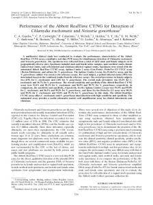
4.10 Experiments of Rate of Progress Approaches In this section, an experiment is presented to show how two progress techniques are accuately predict. This section shows how the approaces accurately predict response time of an application using DynBench introduced by Welch and

Shirazi in [25]. The 'filterl' application (which filters noise from sensed data) in the first sensing path as the task is examined on the variable size of workload scenario. The priority level of the task is assigned to 115 (p(filterl)=115) and 2.33 second arrival rate for T(filterl)=2.33. (Therefore applications in the same path involving 'filterl'

have

same

period.,

that

is,

T(sensorl)=2.33,

T(FM1)=2.33,

T(EDM 1)=2.33, and T(ED 1)=2.33.) The second sensing path denoted to path2 with period T(path2)=0.91, the third sensing path denoted to path3 with period T(path3)=1.73 are used for create contention. The various priority levels, p(ED2)=115 (priority level of ED application in the second sensing path), p(filter3)= 115, p(ED3)=123, p(filter2)=123, p(sensor2)=130, p(FM2)=130,

38

p(FM3)=130, p(EDM2)=130, p(EDM3)=130, and p(sensor3)=130 are assigned in order to create two types of contention, one for due to the same priority tasks and another for due to higher priority tasks. Thirty samples of the response time of 'filterl' are collected and averaged, when workloads of

the path2 are changed dynamically and monotonically.

Workloads of path1 are fixed by 1500, and path3 uses fixed workloads by 800. As shown in Table 4.2, the workload of path2 is increased and dropped significantly until 800 workloads are arrived. Workload then is icreased monotonically until 1200 workloads are reached. is measured using the The response time, hpr,d=Dpr,dl+D,r,d2+C(filterl), same approach for each contention case by RP-1 and RP-2.

Table 4.2 Response time errors using rate of progress approaches.

workload

RP- 1

RP-2

500

0.239947

-0.02276

1300

0.700867

0.017391

800

0.361436

-0.02769

900

0.403667

-0.01022

1000

0.488949

0.00033

1100

0.5265

0.00548 1

1200

0.617074

0.014338

600

0.272931

-0.01562

39

The response time is observed based on the above workload scenario as shown in Fig. 4.2. The RP-1 approach excesses CPU resource up to 70%, while

RP-2 is very accurate, but some very small number of negative error observed.

RP-2 is then useful for control systems, which require accurate prediction.

Response Time Prediction of 'Filterl' by Rate of Progess Approach

1 tresp. t i r e ' 1 I

500

1300

800

900

1000 1100 1200

I

600

workload

Fig. 4.2 Response time comparison of rate of progress approaches.

CHAPTER 5. A WORST-CASE APPROACH TO RESPOINSE TIME ANALYSIS

This chapter presents an approach for calculating Dpredl,Dpred2,and h,,.,d, the outputs of processes 1.1, 1.2 and 1.3 of Fig. 3.3 and Fig. 3.6. This approach extends a worst-case technique as presented in [20] and Klein et al. in [27] to the time sharing round-robin scheduler in order to compute queuing delay due to the prioritized tasks. In addition, the worst-case analysis is used to compare with proress rate approaches as decribed in Chpater 4.

5.1 A Worst-Case Approach for Same Priority Tasks This section analyzes contention that occurs when tasks of

the same

priority share resources. That is, it shows how to calculate Dpredl.We assume that T(A) 2 A,,, and "non-blocking" (no delay caused by priority inversion).

41 The following steps show the iterative process of computing the queuing delay of 'A' due to tasks in 'A*' that have the same priority as 'A'.

Step 1. Compute aro(A), the first approximation of the response time of 'A' uder the assumption of the worst-case contention with same priority tasks.

where, CC(ak) =

r

S(A) * TQ(H)(p(ak)), if S(ak) > S(A)

Note that this approach extends the approach presented by Audsley et al. in [20] to be applicable for time-sharing systems by introducting TQ.

Step 2. Compute ari+l(A)the next approximation of the response time by using the previous approximation. 7

7

ari+ (A) = C (A) +

The ceiling function determines if the period of a task is within the previous approximation. If

all task periods are smaller than the previous

42 approximation, none of the tasks starts during the approximation. Thus, Step 3 performs is necessary for finding the answer.

Step 3. Determine if the approximation is the answer. if (ari(A)== ari+,(A)),then Dpredl(A)= ari(A) - C(A) else increase i and repeat step 2

5.2 Examples of the Worst-Case Approach for Same Priority Tasks This section shows examples of the worst-case approach step by step as described in section 5.1. The worst-case queuing delay for task t l defined in Table 4.1 is used for the first example.

Step 1. Compute aro(tl), the first approximation of response time.

(where, CC(t2) = C(t2) =20, CC(t3)=S(tl)*TQ(H)(p(t3))=1*20=20,

Step 2. Compute arl(tl), the next approximation of the response time.

Step 3. Determine if the approximation is the answer. 70 - 10 = 60 if (aro(A) == arl(tl)), then Dpredl(tl)=

The second example shows the calculation of the worst-case queuing delay for task t8 defined in Table 4.1.

Step 1. Compute aro(t8), the first approximation of response time (are) by adding the time range of other tasks, CC(ak).

= 40 + CC(t9) (where, CC(t9)= S(tl)* TQ(H)(p(t9)) = 3 * 18=54)

Step 2. Compute arl(t8), the next approximation of the response time.

Step 3. Determine if the approximation is the answer. if (aro(t8)== arl(t8)), then Dpredl(t8)= 94 - 40 = 54

5.3 A Worst-Case Approach for Higher Priority Tasks The worst-case analysis is presented in this section to estimate response time of 'A' proposed by Audsley et al. (1991) if

A,,, I T(A). DpredZ,the queuing

delay due to higher priority tasks is estimated using the itterative worst-case approach.

Step 1. Compute aro(A), the first approximation of the response time by summing the execution times of higher priority tasks than 'A'.

Step 2. Compute the next approximation of the response time ari+l(A) = C(A) +

Step 3. Determine if the approximation is the answer

if(ar,+l(A) != arm(A)) and (arm+,< T(A)) then repeat step 2. if(ar,+, (A) > T(A)) then A,, is missed. if(ar,+](A) == ar,,(A)) then Dpred~(A)=arm(A) - C(A).

5.4 An Example of the Worst-Case Approach for Higher Priority Tasks As shown in section 5.3, following example shows step by step the calculation of the queuing delay due to higher priority tasks for task t8 defined in Table 4.1. See Table 4.1.

Step 1. Compute aro(t8), the first approximation of the response time by summing the execution times of higher priority tasks than t8. aro(t8)= C(t8) + C(t5)+ C(t6)+ C(t7) = 40 + 25+10+30 = 105

Step 2. Compute the next approximation of the response time, arl. arl(t8) = C(t8 ) + C(t5) * ceil(ardT(t5)) + C(t6) * ceil(aro/T(t6)) + C(t7)*ceil(ardT(t7)) =40+25*2+10+30=130

Step 3. Determine if the approximation is the answer if (aro(t8) != ar, (t8)), then increase i, and repeat Step 2.

arz(t8) = C(t8) + C(t5) * ceil(arl(t8)/T(t5))+ C(t6) * ceil(arl(t8)/T(t6)) + C(t7)*ceil(arl(t8)/T(t7)) =10+25*2+10+30=130 if (an(@== ar2(t8)),then Dpred2(t8) = arl(t8) - C(t8) = 130-40 =

90.

5.5 Response Time Computation This section combines C(A), Dpredl(A)from section 5.1, and Dpred2(A) from section 5.3 to compute the predicted response time of the task, hpred(A) as shown at 1.3 bubble in Fig. 3.3 and Fig. 3.6. That is, hp,ed(A) = C(A) + Dpredl(A)+ Dpred2(A). Therefore the response time of task t8 used as an examples at section 5.2 and section 5.4 as follows: hpred(t8)=C(t8)+Dpredl(t8) + Dpred2(t8) = 40+ 54 + 90 = 174.

5.6 Experiment of the Worst-Case Approach This section shows how the worst-case approach accurately predicts response time of an application. An experiment design identical to section 4.10 is

47

used, which uses dynamic and monotic workload models. Remember that the 'filterl' application in the first sensing path as a task is examined on the variable contention rate. The response time, hpred=Dpredl+Dpred2+Cr is measured using the worstcase approach for each contention case. From Table 5.1, the worst-case approach excesses resources upto 29 percentage. Overall average error in worst-case apoproach is 20.65 percentage.

Table 5.1 Response time prediction errors.

Following Fig. 5.1 shows how the worst-case and RP-1 approach poorly predicts response time in dynamic environments, while RP-2 predicts versy accurately. More experiments with different experimentaI scenarios are performed in next chapter.

48 -

-

-

--

-

- --

-

-

-

-

-

1

Worst-Case Response Time Prediction of 'Filterl'

+resp t~rne RP-1

*worst-case +RP-2 - -

500

1300

800

900

1000

1100

1200

-

600

workload

Fig. 5.1 Response time prediction by worst-case approach

1

-

CHAPTER 6. SYNTHESIZED APPROACHES TO RESPONSE TIME PREDICTION

This chapter synthesizes three approaches presented at previous chapters 4 and 5 in order to predict response time of the application and exams the synthesized approaches using experiments.

6.1 Synthesizing Contention Analysis Approaches In this section, the final prediction techniques

under dynamic

environments by synthesizing previous approaches are presented. As the predicted response time of 'A' , h pred(A)=C(A)+ Dpredl(A) + Dpred2(A),nine combinations from 3 different approaches (RP-1 ,RP-2, Worst-Case) are examined. The following Table 6.1 shows possible choices (sl to s9) as synthesized approaches. The same techniques used for computing Dpredland Dpred2 are s l , s5, and s9. The s l approach computes response time by adding C(A), Dpredlfrom the worst-case approach and Dpred2from the worst-case approach. The s2 approach is

50 synthesized by RP-1 for Dpredland by the worst-case for Dpred2. The s3 approach is synthesized by RP-2 for Dpredland by the worst-case for Dpred2The s4 approach is synthesized by the worst-case approach for Dpredland by RP-1 for DpledZThe s5 approach is synthesized by the RP-1 for Dpredland by RP-1 for Dplrd2. The s6 approach is synthesized by RP-2 for Dpredland by RP-1 for Dpred2. The s7 approach is synthesized by the worst-case approach for Dpredland by RP-2 for DpledZThe s8 approach is synthesized by the RP-1 for Dpredland by RP-2 for Dplrd?Finally, the s9 approach is synthesized by RP-2 for Dpredland by RP-2 for Dpr.ed2.

Table 6.1 The synthesized cases for the final response time prediction. same priority different priority Worst-case

worst-case

RP- 1

RP-2

s1

s2

s3

RP- 1

s4

s5

s6

RP-2

~7

SS

s9

Table 6.2 shows the response time of task t8 used in chapters 4, and 5 as an example of combining two queuing delays with the execution time of t8. From Table 6.2, we can deduce that the synthesized approach, s4, appears to be the most pessimistic approach for estimation of response time. The s9 calculates the smallest response time.

Table 6.2 The synthesized response time analysis. same priority different priority

worst-case

RP- 1

RP-2

Worst-case

184

177.8

135.5

RP- 1

191.9

185.5

143.4

RP-2

114.6

108.4

71.1

6.2 Experiments of Synthesized Approaches In this section, experiments of response-time prediction approaches are discussed to verify accuracy of each technique with different case of environmental conditions.

6.2.1 Measurement Analysis In order to measure accuracy of each technique, the error and the statistical significace must be considered. To do this, observed response time of 'A', denoted to hOb,(A), must be accurately measured. The measurement error of

hOb,(A) can be caused by two factors. The first comes from the technique that is used to collect the measurements. This error will be consistent whenever a measurement is collected. The second error is due to the phasing problem of different applications on the same host. Introducing fluctuation between the samples for the same workload

52 depends on the application combination running on the host and also changes when workload changes. For example, two applications could run on the same host with different periods. However, each application will have a different contention at each cycle due to the changing of arrival time. This error demonstrates periodic characteristic. The following steps show how experiments are done to collect AObS(A)

Step 1. Choose several level of workload that we want to quantify the sampling error from the scenario file.

Step 2. Run the software system twice and collect more than 30 samples for each.

Step 3. Compute the error range with confident level (95% confident level is used: a=0.05, z=1.96) from two groups using ZTEST. The zvalue is calculated as follows:

u. - u- - E

53 where ui is mean of group i,

02, is

variance of group i, ni is number of

samples in group i.

Therefore, based on the Step 3, the error between the mean of distribution and the mean of the observed data can be examined. If the error is bigger than the error range ( r ) , this approach rejects the observed data.

6.2.2 Experiment on Gradually Increased Workload Scenario In experiment (I), the accuracy of each technique for the response time prediction of an application was examined on a gradually increased workload scenario. The 'ED1' (Evaluate and Decide) application of sensing path 1 in DynBench was used as the task 'A', which is a program that evaluates data and decides action trigerring for the data. The prioiry level of ' E D l ' is assigned to 115 (p(ED1)=115) with 1500 workloads and 0.83 second arrival rate for all applications in sensing path 1 (T(pathl)=0.83), and two sensing paths 2 and 3 are used for contention with T(path2)=1.17 and T(path3)=0.5 1, respectively. Hence, applications in the sensing path have same periods as the path. The priority levels for the 'ED2' in sensing path 2 (p(ED2)) is assigned to 115, p(ED2)=115, and p(filter3)= 115, p(ED3)=123, p(filter2)=123, and 130 priority level is assigned to all other applications in sensing path 2 and 3. The workload of sensing path 3 is fixed by 500, and that of sensing path 2 is increased by 100 every 30 seconds.

54 The Experiment Generator (EG), a SW tool for DynaBench to produce dynamic experiment scenario, reads each line as shown in Fig. 6.1 (a) and sends to the sensor application the command at the absolute time defined in the first column. The sensor is started with inital 1000 workloads for path 2. At 1 minute 20 second after the EG program starts, it asks the sensor to add 100 additional workloads.

0:01:20:0: 0:02:40:0: 0:04:00:0: 0:05:20:0:

sensor2 sensor2 sensor2 sensor2

add add add add

tracks tracks tracks tracks

100 //initial workload = 1000 100 100 100

(a) Experiment file for gradually increased workload

Gradually Increased Experiment File

-

1500

;1000 C

m

g 0

500

3 0 - m c n m b - m a m b - l & - l g p b - m N P ~ ~ C U m c o m - 2 ? ? F , Z , , m m m m

time

(b) Experiment file graph Fig. 6.1 Gradually increased experiment file.

55

6.2.2.1 Response Time Prediction for 'ED' Before validation of the response time prediction of the 'ED17 by each technique, the error range is computed as shown in formula (6-1) at 95 percent confidence level to find out measurement error occurred. Table 6.3 shows that the error range between the observed response time and the predicted response time by different workload cases applied in path2 is computed to compare with the observed data error. The two pre-collected groups are tested with exactly the same scenario as defined in Fig. 6.1. The first column in Table 6.3 is the workloads of path2. The second is the error range for the 'ED1'.

Table 6.3 Error range of 'ED1' at 95 percent confidence level. workload of path2

error range

1000

0.008641

1100

0.013575

1200

0.014784

1300

0.01 1868

1400

0.007453

Fig. 6.2, Table 6.4 and Table 6.5 show comparison of each technique. The s3 is

closest to the observed response time (denoted Aobs(ED1)). The s l

(combination of two worst-case analyses) overuses 19 percent CPU resource, while the s9 only exceeds 1.6 percent resource usage. Table 6.4 tells predicted

56 repsonse time for each synthesized approach, and Table 6.4 shows error between hob,@ 1) and hpred(EDl).

Response Time Prediction of 'ED1' by Synthesized Approaches

' +resp. time s1 52 53

+s4 -e- 55 +s6 1000

1100

1200

1300

1400

workload

Fig. 6.2 Response time prediction by synthesized techniques.

Table 6.4 Response time prediction of 'ED1' by synthesized approaches.

57

Table 6.5 Comparison of response time error of 'ED1'.

The error range shown in the Table 6.5 can be applied in order to verify each technique's significance within confidence level. In the experiment, no measurement error occurred. The s9 approach is most accurate but the s l performs worst in terms of accuracy. Overall error of each approach in terms of resource utilization is as follows: 19.6 percentage for s l , 16.2 percentage for s2, 13 percentage for s3, 13.4 percentage ,for s4, 9.9 percentage for s5, 6.8

percentage for s6, 7.7 percentage for s7, 4.2 percentage for s8, and 1.1 percentage for s9 are observed.

6.2.3 Experiment on Dynamically Changed Workload Scenario The 'filterl' application of sensing path 1 in DynBench is used as the task 'A' examined on a dynamically changed workload scenario. The priority level of

the task is assigned to 115 (p(filterl)=115) with 1500 workloads and 0.83 second arrival rate for all applications in sensing path 1 (T(pathl)=0.83), and two sensing

58 paths 2 and 3 are used for contention with T(path2)=1.17 and T(path3)=0.51, respectively. The priority levels p(ED2)=115, p(filter3)=115,

p(ED3)=113,

p(filter2)=113, 130 for priority level of all other applications in sensing path 2 and 3 are assigned. The workload of sensing path 3 is fixed by 800, and that of sensing path 2 is suddenly increased to 1300 by adding 800 workloads at 1 minute 20 seconds; it drops by 600 at 2 minutes 40 seconds; it adds 700 again at 4 minutes, and drops

500 at 5 minutes 20 seconds. See Fig. 6.3 (a) and (b).

add remove add remove

0:01:20:0: sensor2 0:02:40:0: sensor2 0:04:00:0: sensor2 0:05 :20:0: sensor2

tracks tracks tracks tracks

800 //initial workload = 500 600 700 500

(a) Dynamic workload experiment file

Dynamically C h a n g e d E x p e r i m e n t File

=. -+ g 3

1600 1400 1200 1000 800 600 400 200 0

-

m ~

m

g

m

r

r

.

.

m -

~ ~ ~ -

~

m -

m r a m N N tim e

.

N

-

m f N

m a m

m m m

r m

. m

(b) Dynamic workload scenario graph

Fig. 6.3 Dynamically changed workload scenario.

m

m w

r

n

59

6.2.3.1 Response Time Prediction for 'filter' First, to determine the accuacy of the observed data, the error range was computed by formula (6-1) at 95 percent confidence level from collections as shown in the Table 6.6. The error range of workload 1400 as shown in Table 6.6 was smaller than 1300 workloads. This implies that smaller variances at 1400 workloads are obtained than at 1300 workloads. The first column in Table 6.6 is the workloads for path2. The second is the error range for the 'filterl'. It shows various contentions are emloyed by changing workload of path2.

Table 6.6 The error range of 'filterl' on dynamically changed workload scenario. workload of path2

error range

500

0.005388

700

0.004836

900

0.008289

1300

0.024508

1400

0.009678

Fig. 6.4 and Table 6.7 shows the response time prediction by synthesized approaches. The response time predictions by s9 is still superior to any others as shown in Fig. 6.4. The s l performs worst in this scenario as well.

- -

-

-

-

-

Response Time Prediction of 'Filter1' on Dynamic Scenario --

--

--

--t resp. time

s1 s2 s3 s4

+

500

1300

700

1400

900.

time

workload --

-

-

--

--

-

-

Fig. 6.4 Response time prediction by synthesized approaches on dynamically changed workload.

Table 6.7 Error comparisons by each technique.

workload

sl

s2

s3

s4

s5

S6

s7

s8

s9

500

0.081 0.08 0.071 0.067 0.066 0.057 -0.001 -0.002 -0.011

1300

0.241 0.203 0.005 0.171 0.133 0.166 0.085 0.047 0.005

700

0.117 0.112 -0.004 0.091 0.086 0.096 0.018 0.013 -0.004

1400

0.277 0.225 0.018 0.198 0.146 0.19 0.11 1 0.059 0.018

900

0.147 0.13 -0.003 0.108 0.091 0.115 0.03 0.013 -0.004

61 Table 6.7 shows the errors can be evaluated to find which technique is significant. The s9 technique is significant but not in all cases. No case of measurement error occurred in the experiment. Overall error in terms of resource ~ltilizatio~zis as follows: 17.3 percenatge for s l , 15 percentage for s2, 1.7 percentage for s3, 12.7 percentage for s4, 10.4 percentage for s5, 12.5 percentage ,for s6, 4.9 percentage for s7, 2.6 percentage for s8, and 0.08 percentage for s9 are observed.

6.2.4 Experiment on Combined Scenario

This experiment is done by combining the previous two scenarios. The 'filterl' in sensing path1 is also used as the task 'A'. The different contention model is applied by changing periods of other applications. The prioiry level of the task is assigned to 115 (p(filterl)=115) with 1500 workloads and 2.33 second arrival rate for all applications in sensing path 1 (T(pathl)=2.33), and two sensing paths 2 and 3 are used for contention with T(path2)=0.91 and T(path3)=1.73, respectively. The priority levels, p(ED2)=115, p(filter3)=115,

p(ED3)=123,

p(filter2)=123, and 130 for priority level of all other applications in sensing path 2 and 3 are assigned. In Fig 6.5, a new combined experiment scenario is defined. At 1 minute 20 seconds after EG starts, EG sends the first line command to add 800 workloads, and removes 500 workloads at 2 minute 40 seconds. There is a gradual workload

62 increase of 100 each time, before which finally drops to 600 workloads which is significant.

0:01:20:0: 0:02:40:0: 0:04:00:0: 0:05:20:0: 0:06:40:0: 0:08:00:0: 0:09:20:0:

sensor2 sensor2 sensor2 sensor2 sensor2 sensor2 sensor2

add remove add add add add remove

tracks tracks tracks tracks tracks tracks tracks

800 //initial workload = 500 500 100 100 100 100 600

(a) Experiment file for combined scenario

Combined Experiment File 1400

a SO g

1200 1000 800 600 400 200 0 - a r . ~ $ - a t . m m - a r . m m - c T (3 r. 7 ? z wm 0m 8 % G % %

~

%

time

(b) Experiment scenario graph for combined workload

Fig. 6.5 Experiment file for combined workload scenario.

~

63 6.2.4.1 Response Time Prediction for 'filter'

In this section, the 9 synthesized approaches used to predict the response time of the filter on the combined workload scenario are shown in Fig. 6.5. The error range by formula (6-1) is illustrated in Table 6.8. As shown in Table 6.8, error range is relatively longer when workload of others is changed dynamically (see 800, and 1300 workload cases) than when workload changes follow a monotonic model (see 900,1000,1100,and 1200 workload cses).

Table 6.8 The error range of filter on the combined workload scenario at 95 percent confident level.

The combined scenario brings more variations in response time prediction, even though CPU is only used up to 65 percent. The s5 (RP-1 & RP-1) is predict

64 response time most poorly in this experiment, while s9 predicts still accurately. Fig. 6.6 and Table 6.9 show the comparison of each synthesized prediction technique. Overall error in terrns of resource utilization is obtained .from Table 6.9 as follows: 20 percenatge for s l , 29.3 percentage for s2, 16.2 percentage for s3, 35.8 percentage for s4, 45.1 percentage for s.5, 32 percentage for s6, 3.3 percentage for s7, 12.6 percentage for s8, and 0.5 percentage for s9 are ovserbed.

1

Response Time Prediction of 'Filter1' I

--t resp. tlme

s3

-m- s4

Fig. 6.6 Response time prediction by synthesized techniques.

65

Table 6.9 Comparison of response time errors by synthesized techniques.

From the three different experiments presented in section 6.2, there is no measurement error observed under the 95% confidence interval. The s9, probabilistic contention analysis technique, PR-2, can accurately predict response time of an application on a, while the s l involving the worst-case analysis poorly predicts response times. Therefore, these experiments for the dynamic real-time systems give strong analysis that the worst-case analysis poorly utilizes computational resources, and new approaches can predict response time accurately with the dynamic environment constraints using current utilization. This suggests that schedulability of tasks can be predicted without using any real-

66 time operating system components. The s7 and s8 might be useful schedulability

analysis method for hard real-time constarints rather than the worst-case.

CHAPTER 7. CONCLUSION

In this final chapter, the conclusion and suggestions for future study are presented.

7.1 Thesis Summary

The main contribution of this thesis is certification of real-time performance for dynamic real-time applications. An erroneous system cerification can lead to a catastrophe in a real-time system. The certification approach taken is schedulability analysis (SA) for a feasible allocation of computing resources on hosts that run thesolaris operating system. This is accomplished with a mathematical model and accurate response time prediction for a periodic, dynamic, distributed real-time applications. The SA method is also applicable for hosts that use time-sharing round-robin schedulers. Experimental results validate the SA techniques. The s9 probabilistic contention analysis technique, employing RP-2, accurately predicts response time of an application under the dynamic environments as compared with the s l

68 involving the worst-case analysis which poorly predicts response times. The overall error of s9 (progress rate approach) in resource utilization was 0.4 percentage, while 18 percentage is observed for error of s l (worst-case approach).

7.2 Future Study This research opens the possibility for additional interesting research. First, there is the topic of certification for an event-driven real-time application which is periodic as well as aperiodic. Second, a new research area derived from this study is the determination of confidence levels of certification, which will be analyzed by mathematical methods with an upper bound, or error.

In addition, management of network bandwidth by a resource manager presents a challenge for the future because the end-to-end QoS of distributed applications is highly dependant on communication delay. QoS balance rather than host load-balance should also be considered as a subject for future study as complex real-time systems require the handling of multiple QoSs of other applications or paths.

BIBLIOGRAPHY

[I] Liu, C. L., and J.W. Layland, "Scheduling algorithms for multi-programming in a hard-real-time environment", Journal of the ACM, Vol. 20: 46-61, 1973. [2] Ramamritham, J.A. Stankovic and W. Zhao, "Distributed scheduling of tasks with deadlines and resource requirements," IEEE Transactions on Computers, Vol. 38(8), 110-123, August 1989. [3] Haban, D. and K. G. Shin, "Applications of real-time monitoring for scheduling tasks with random execution times", IEEE Transactions on Software Engineering, Vol. 16(12): 1374-1389, 1990. [4] Tia, T. S., Z. Deng, M. Shankar, M. Storch, J. Sun, L.C. Wu and J.W.S. Liu, "Probabilistic performance

guarantee

for real-time tasks

with

varying

computation times", Proceedings of the 1" IEEE Real-Time Technology and Applications Symposium, IEEE Computer Society Press: 164-173, 1995.

[ 5 ] Lehoczky, John P., "Real-Time Queueing Theory", Proceedings of IEEE Real-Time Systems Symposium, IEEE CS Press : 186-195, 1996. [6] Abeni, L. and G. Buttazzo, "Integrating multimedia applications in hard realtime systems", Proceedings of the 19"' IEEE Real-Time Systems Symposium, IEEE Computer Society Press: 3-13, 1998.

70 [7] Stewart, D.B. and P.K. Khosla, "Mechanisms for detecting and handling timing errors", Communications of the A C M , Vol. 40(1): 87-93, 1997.

[8] Puschner, Peter and Alan Bums, "A Review of Worst-Case Analysis", The Internatiorzal Journal of Time-Critical Computing Systems, Vol. 18: 115-128,

2000.

[9] Atlas, A., and A. Bestavros, "Statistical rate monotonic scheduling", Proceedings of the 19"' IEEE Real-Time Systems Symposium, IEEE Computer

Society Press: 123-132, 1998.

[lo] Welch, L.R and M.W. Masters, "Toward a Taxanomy for Real-Time Mission-Critical systems", Proceedings of the First International Workshop orz Real-Time Mission- Critical Systems, 1999.

[ l l ] Liu, J.W.S,

K,-J. Lin, W.-K. Shih Yu, J.-Y. Chung, and W. Zhao,

"Algorithm or Scheduling Imprecise Computations", IEEE Computer,

Vol.

24(5): 58-68, 1991.

[12] Thuel, Sandra R. and John P. Lehoczky, "Algorithms for Scheduling Hard Aperiodic Tasks in Fixed-Priority Systems using Slack Stealing", Proceedings of IEEE Real-Time Systems Symposiunz: 22-33, 1994.

[13] Jensen, Douglass, C. Douglas Locke, and Hideyuki Tokuda, "A Time Driven

Scheduling Model for Real-Time Operating Systems", Proceedings of IEEE Real-Time Systems Symposium: 112-122, 1985.

71 [14] Chen, Ken, "A scheduling Algorithm for Tasks Described by Time Value Function", Real-Tirne Systems, Vol. 10: 293-3 12, 1996.

[IS] Shirazi, B., A. R. Hurson, and K. Kavi, Scheduling and Load Balancing in

Parallel and Distributed Systems, IEEE Press, 1995. [I61 Buhr, Raymond J.A. and Donald L. Bailey, An Introduction to Real-Time

Systems from Design to Networking with C/C++. Prentice Hall, 1999. [17] Klein, Mark, Thomas Ralya, Bill Pollak, Ray Obenza, and Michael G. Harbour, A Practitioner's Handbook for Real-Time Analysis: Guide to Rate

Monotonic Analysis for Real-Time Systems. Kluwer Academic Publishers, 1993.

[18] Sha, L., M. H. Klein, and J.B. Goodenough, Rate monotonic analysis for

real-time systems in Scheduling and Resource Management, Kluwer: 129-156, 1991.

[19] Chu, W.W., "Task Response time Model & its applications for real-time distributed processing system", Proceedirzgs of

IEEE Real-Time Systevls

Sy~1posiunz:225-236, 1983.

[20] Audsley, Neil C., "Deadline Monotonic Scheduling", (Report YCS-90-146), Department of Computer Science, York University , 1990.

[21] Chatterjee, Saurav and Jay Strosnider, "Distributed Pipeline Scheduling: A Framework for Distributed, Heterogeneous Real-Time System Design7', In the

Covzputer Journal, British Computer Society, Vol. 38, No. 4, 1995.

[22] Welch, L.R., A.D. Stoyenko,and T.J. Marlowe, "Response Time Prediction for Distributed Processes Specified in CaRT-Spec", Control Eng. Practice, Vo1.3, NO. 5 : 651-664, 1995.

[23] Brandt, Scott, Gary Nutt, Toby Berk, and James Mankovich, "A Dynamic Quality of Service Middleware Agent for Mediating Application Resource Usage", Proceedings of IEEE Real-Time Systems Symposium: 307-317, 1998.

[24] Welch, L.R., B. Ravindran, B.Shirazi and C. Bruggeman, "Specification and Analysis of Dynamic, Distributed Real-Time Systems", Proceedings of the 19'" IEEE Real-Time Systems Symposium, IEEE Computer Society Press : 72-81, 1998.

[25] Welch, L. R. and B. Shirazi, 1999. "A Dynamic Real-Time Benchmark for Assessment of QoS and Resource Management Technology". IEEE Real-time Application System.

[26] Pressman, Roger S., Software Engineering: A Practitioner's Approach. McGraw-Hill Companies, 1996.

[27] Kleinrock, Leonard, Queuing Systems. Vol. 1. A Wiley-Interscience Publication, 1975

[28] IBM Corporation, IBM Load Leveler User's Guide, 1993. [29] Foster, Ian, C. Kesselman, "Globus: A Metacomputing Infrastructure Toolkit. Intl J. Supercomputer Applications", 1l(2): 115-128, 1997.

73 [30] Becker, Donald J., Thomas Sterling, Daniel Savarese, John E. Dorband, Udaya A. Ranawak, Charles V. Packer, "BEOW ULF: A PARALLEL WORKSTATION FOR SCIENTIFIC COMPUTATION", Proceedings of Internationul Conjerence on Parallel Processing, 1995.

[31] Czajkowski, Karl, Ian Foster, Carl Kesselman, Stuart Martin, Warren Smith, Steven Tuecke, "A Resource Management Architecture for Metacomputing Systems", Proc. IPPS/SPDP '98 Workshop on Job Scheduling Strategies for Parallel Processing, 1998.

[32] Welch, Lonnie R., Behrooz A. Shirazi, Binoy Ravindran, and Carl Bruggeman, "DeSiDeRaTa: QoS Management Technology for Dynamic, Scalable, Dependable, Real-Time Systems7',IFAC: 7-1 1, 1998.

[33] Burns, Frank, Albert Koelmans, and Alexandre Yakovlev, "WCET Analysis

of Superscalar Processors Using Simulation With Coloured Petrinets", The International Journal of Time-Critical Computing Systems, Vol. 18: 275-288,

2000.