cfd algorithms in high performance fortran - CiteSeerX

NPAC Technical Report SCCS 737

CFD ALGORITHMS IN HIGH PERFORMANCE FORTRAN K.A.Hawick, E.A.Bogucz,y A.T.Degani,z G.C.Fox x G.Robinson,{ Northeast Parallel Architectures Center, 111 College Place, Syracuse, NY 13244-4100 k

Abstract

Although parallel and distributed machines have shown the promise of ful lling this objective, the potential of these machines for running large-scale production-oriented CFD codes has not been fully exploited yet. It is expected that such computations will be carried out over a broad range of hardware platforms thus necessitating the use of a programming language that provides portability, ease of maintainance for codes as well as computational eciency. Until recently, the unavailability of such a language has hindered any comprehensive move toward porting codes from mainframes and traditional vector computers to parallel and distributed computing systems. High Performance Fortran (HPF)2 is a language definition agreed upon in 1993, and being widely adopted by systems suppliers as a mechanism for users to exploit parallel computation through the data-parallel programming model. HPF evolved from the experimental Fortran-D system3 as a collection of extensions to the Fortran 90 language standard4 . We do not discuss the details of the HPF language here as they are well documented elsewhere5 , but simply note that the central tenet of HPF and data-parallel programming is that program data is distributed amongst the processors' memories in such a way that the \owner computes" rule allows the maximum computation to communications ratio. Language constructs and embedded compiler directives allow the programmer to express to the compiler additional information about how to produce code that maps well to the available parallel or distributed architecture. In this manner, the code runs fast and can make full use of the larger (distributed) memory. We have already conducted a preliminary study of the general suitability of the HPF language for CFD6 using experimental HPF compilation systems developed at Syracuse and Rice, and with the growing availability of HPF compilers on platforms such as Digital's Alphafarm we are able to describe speci c coding issues. Unfortunately, we are unable to report performance timing gures since we are working with an early release of a

We evaluate the High-Performance Fortran (HPF) language for expressing and implementing algorithms for Computational Fluid Dynamics (CFD) applications on high performance computing systems. In particular we discuss: implicit methods such as the ADI algorithm, full-matrix methods such as the panel method, and sparse matrix methods such as conjugate gradient. We focus on regular meshes, since these can be eciently represented by the existing HPF de nition. The codes discussed are available on the World Wide Web at http://www.npac.syr.edu/hpfa/ alongwith other educational and discussion material related to applications in HPF.

1. Introduction Successful implementations of envisioned multidisciplinary analysis and design for large-scale aerospace systems require High Performance Computing and Communications (HPCC) technology to provide faster computation speeds and larger memory. HPCC is already important for rapid and cost-eective execution of simulation codes in individual disciplines and is even more necessary for the simultaneous execution of the various components of multidiscipline design codes such as computational uid dynamics (CFD), computational electromagnetics (CEM)1 , thermodynamics and structural models.  Senior Research Scientist; HPF Applications Project Leader; Member, AIAA. y Associate Director; Associate Professor; Associate Chairman, Department of Mechanical, Aerospace and Manufacturing Engineering, Syracuse University. Member, AIAA. z Alex G. Nason Research Fellow, Member, AIAA. x Director; Professor, Computer Science and Physics, Syracuse University; Member, AIAA. { Research Scientist k This work sponsored, in part, by ARPA 0 Copyright c 1995 by A. T. Degani. Published by the American Institute of Aeronautics and Astronautics, Inc. with permission.

1 American Institute of Aeronautics and Astronautics

where  is the central-dierence operator. Denoting 2 as the averaging operator over twice the mesh interval, the central dierence operator, , in terms of 2 is given by  2 = 2(?1 + 2). This identity may be used to express equation 3 in two alternative ways, viz. ( ) y2 2 2x ?
x2 +
y2 = f ? 2 (4)
x2 ;

proprietary HPF compiler. To illustrate the main ideas of data distribution and communication in an HPF code, we implement the ADI algorithm and demonstrate how con icts between the optimal data decomposition and the computational structure of the algorithm may be resolved. Full matrix algorithms can also be implemented in HPF, and we illustrate these ideas with a panel method code. Sparse matrix methods such as the conjugate gradient method are not trivial to implement eciently in HPF at present. The diculty is an algorithmic one rather than a weakness of the HPF language itself. We demonstrate this idea with a conjugate gradient code, where the resulting sparse matrix can be solved iteratively, reducing the linear algebra component to essentially one of matrix-vector multiplies. Practical implementations for large problems require the matrix to be stored as a sparse system, and the resulting indexing into the packed storage scheme is not simple to implement in a scalably ecient manner. For the purposes of carrying out multi-disciplinary simulations which include CFD, it is generally of prime importance to achieve a given level of numerical accuracy for a given size of system in the shortest possible time. Consequently, there is a tradeo between rapidly converging numerical algorithms that are inecient to implement on parallel and distributed systems, and more slowly converging and perhaps less numerically \interesting" algorithms that can be implemented very eciently7 . We illustrate these ideas in the implementation of the algorithms considered here.



x2 ? 2  = f ? 22y : (5)
x2
y2
y2 If we restrict our attention to a second-order accurate formulation, then, for each i, 1  i  Nx , equation 4 de nes a tridiagonal system of equations subject to Dirichlet boundary conditions at j = 0 and j = Ny + 1. In the x-sweep of the ADI algorithm, i is varied from 1 to Nx and at each i location, equation 4 is solved to obtain updated values of for all j. Subsequent to the completion of the x-sweep, a y-sweep is initiated by varying j from 1 to Ny , but now, the tridiagonal system in equation 5 is solved subject to Dirichlet boundary conditions at i = 0 and i = Nx + 1. An x-sweep followed by a ysweep completes one ADI iteration. Figure 1 shows the important code fragments for the sequential implementation of the ADI method written in FORTRAN 90. The tridiagonal coecient matrix along with the righthand side of equations 4 and 5 are evaluated in the array C(1:4,:). This array is then passed to the subroutine THOMAS which uses the well-known Thomas algorithm to solve the tridiagonal system of equations. The variables BCLFT, BCRHT, BCBOT and BCTOP are the Dirichlet conditions on the four sides of the boundary and are assumed constant. The coecient matrix for the Poisson equation is constant and need not be formed every iteration; however, for nonlinear problems, the coecient matrix must be evaluated every iteration and the code structure in gure 1 re ects this general situation. Note that in both the x- and y-sweeps, the updated values of are used immediately in forming the tridiagonal system of equations at the next station. Prior to discussing the ADI implementation in HPF, we rst address the broader issue of data-parallel execution and data dependency. To this end, consider the evaluation of the right-hand side C(4,:) in the xsweep. The presence of PSI(I-1,1:NY) within the DO loop causes a data dependency which prohibits dataparallel execution. For nonlinear problems, the evaluation of the coecient matrix may also introduce data dependency. A similar argument also holds for the ysweep. Clearly, the sequential code in gure 1 must be modi ed to enable data-parallel execution, and the simplest alternative is to form all the coecient matrices rst before solving any of the tridiagonal system of equations. This modi cation is shown in the code fragment in gure 2. In eect, the data dependency shown

2. Alternate Direction Implicit The Alternate Direction Implicit (ADI) method is an iterative technique commonly used to solve timedependent nonlinear set of equations. However, in order to highlight the salient algorithmic features of the ADI implementation in HPF, we consider the simple twodimensional Poisson equation for illustrative purposes. Let

r2 = f on = (0; 1)  (0; 1);

(1) = g on @ ; (2) where, for simplicity, we assume Dirichlet boundary conditions on . The domain is discretized into Nx +1 and Ny +1 equal intervals along the x and y directions, respectively, and the grid indices vary as 0  i  Nx +1 and 0  j  Ny + 1. A nite-dierence discretization of equation 1 yields (

x2 + y2
x2
y2

)

= f;

(3) 2

American Institute of Aeronautics and Astronautics

...

...

PROGRAM ADI_SEQUENTIAL declarations, interfaces and initializations ... DO ITER = 1,ITERMAX ! begin iteration loop DO I = 1,NX !x sweep C(1,1:NY) = DY2INV C(2,1:NY) = -2.0_FPNUM*(DX2INV+DY2INV) C(3,1:NY) = DY2INV C(4,1:NY) = F(I,1:NY) - & DX2INV*(PSI(I+1,1:NY)+PSI(I-1,1:NY)) CALL THOMAS (NY,C,BCBOT,BCTOP,PSI(I,0:NY+1)) END DO DO J = 1,NY !y sweep C(1,1:NX) = DX2INV C(2,1:NX) = -2.0_FPNUM*(DX2INV+DY2INV) C(3,1:NX) = DX2INV C(4,1:NX) = F(1:NX,J) - & DY2INV*(PSI(1:NX,J+1)+PSI(1:NX,J-1)) CALL THOMAS (NX,C,BCLFT,BCRHT,PSI(0:NX+1,J)) END DO check convergence ... END DO END

DO I = 1,NX C(1,I,1:NY) C(2,I,1:NY) C(3,I,1:NY) C(4,I,1:NY)

...

...

END DO solve a set DO J = 1,NY C(1,J,1:NX) C(2,J,1:NX) C(3,J,1:NX) C(4,J,1:NX)

= = = =

!x sweep DY2INV -2.0_FPNUM*(DX2INV+DY2INV) DY2INV F(I,1:NY) - & DX2INV*(PSI(I+1,1:NY)+PSI(I-1,1:NY))

of tridiagonal system of equations !y sweep = DX2INV = -2.0_FPNUM*(DX2INV+DY2INV) = DX2INV = F(1:NX,J) - & DY2INV*(PSI(1:NX,J+1)+PSI(1:NX,J-1))

END DO solve a set of tridiagonal system of equations

Figure 2: Modi cation of x- and y-sweeps to enable data-parallel execution

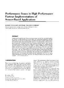
ily introduce data dependency. On the other hand, if the coecient matrix and the right-hand sides are evaluated as suggested in gure 2, the resulting set of the tridiagonal system of equations may be solved in any order. Thus, the order of execution in the x-sweep is independent of I, and, for the y-sweep, is independent of J. It then follows that the optimal data distribution for the x- and y-sweeps is as shown in gure 3 where, for illustrative purposes, a machine with four processors is assumed. The ADI method is a simple example that serves to illustrate that the optimal data distribution for ecient execution is, in general, dierent for various sections of the code. One possible solution to this problem is to redistribute the data back and forth between the two layouts shown in gure 3, and this is considered Figure 1: Sequential ADI solver for the two-dimensional next in the implementation of the ADI method in HPF. Poisson equation ...

SUBROUTINE THOMAS (NK,C,Z0,ZN,Z) declarations ... D(1,0) = 0.0 D(2,0) = Z0 DO K=1,NK D(1,K) = -C(1,K)/(C(2,K) + C(3,K)*D(1,K-1)) D(2,K) = (C(4,K)-C(3,K)*D(2,K-1))/ & (C(2,K) + C(3,K)*D(1,K-1)) END DO Z(NK+1) = ZN DO K=NK,1,-1 Z(K) = D(1,K)*Z(K+1) + D(2,K) END DO Z(0) = Z0 RETURN END

within the DO loops in gure 1 is removed by decomposing each DO loop into two: (i) in the rst loop, the coecient matrix is formed using the values of PSI from the previous sweep, and (ii) in the second loop, which is not shown in gure 2, a set of tridiagonal system of equations are solved. It may be noted that C needs to be promoted to a three-dimensional array which increases memory requirements | a common feature of data-parallel constructs. Although data-parallel execution has been enabled by the modi cations shown in gure 2, it should be noted that the convergence characteristics of the ADI algorithm have also been altered and this issue is discussed subsequently. An important aspect of writing code in HPF is determining the optimal data distribution among the processors. Consider the thomas algorithm in gure 1. The two loops in K correspond to forward and backward substitution and use recursive relationships which necessar-

P0 P1 P0

P1

P2

P3 P2 P3

(a) x-sweep

(b) y-sweep

Figure 3: Optimal data distribution for the x- and ysweeps of the ADI method. Figure 4 shows a fragment of the HPF code, where the directives are speci ed by `!HPF$'. The processors P are arranged in a one-dimensional array and the number of processors, NUMPROCS, is speci ed in a module 3

American Institute of Aeronautics and Astronautics

not necessary with the HPF directive REDISTRIBUTE, we restrict our attention henceforth to the case where Nx = Ny . ... The x-sweep is immediately followed by a TRANSPOSE !HPF$ PROCESSORS P(NUMPROCS) of PSI. In this fashion, the distribution of the transpose !HPF$ TEMPLATE TEMPPSI(0:NMAX+1,0:NMAX+1) PSI(J,I) according to the data layout in gure 3(a) is !HPF$ TEMPLATE TEMPC(4,0:NMAX+1,0:NMAX+1) equivalent to the distribution of PSI(I,J) in gure 3(b). !HPF$ DISTRIBUTE TEMPPSI(BLOCK,*) !HPF$ DISTRIBUTE TEMPC(*,BLOCK,*) Thus the stage is set for the data-parallel execution of !HPF$ ALIGN with TEMPPSI :: PSI,F,FT the y-sweep. In comparing the DO loop in the y-sweep !HPF$ ALIGN with TEMPC :: C in gures 2 and 4, note that the arrays on the righthand side in the HPF implementation are transposes FT = TRANSPOSE(F) !transpose F and store in FT of those in shown in gure 2. The forcing function of DO ITER = 1,ITERMAX ! begin iteration loop the Poisson equation, represented by the array F, needs DO I = 1,NX !x sweep to be transposed only once, and, in the implementation C(1,I,1:NY) = DY2INV here, the transpose is stored in the array FT. Note that C(2,I,1:NY) = -2.0_FPNUM*(DX2INV+DY2INV) C(3,I,1:NY) = DY2INV in both the x- and y-sweeps, communication is required C(4,I,1:NY) = F(I,1:NY) - & along the processor boundaries in order to evaluate the DX2INV*(PSI(I+1,1:NY)+PSI(I-1,1:NY)) right-hand side in C(4,:,:). Finally, the subroutine END DO THOMAS (not shown) is modi ed to include an outer DO CALL THOMAS (NX,NY,C,BCBOT,BCTOP,PSI) loop which steps along the direction of the sweep. PSI = TRANSPOSE(PSI) !transpose after x-sweep We now return to the issue of comparing the converDO J = 1,NY !y sweep gence characteristics of the data-parallel and sequential C(1,J,1:NX) = DX2INV implementations. Since the former does not use the upC(2,J,1:NX) = -2.0_FPNUM*(DX2INV+DY2INV) dated values within a sweep, it may be expected that its C(3,J,1:NX) = DX2INV C(4,J,1:NX) = FT(J,1:NX) - & convergence rate is inferior to that of the latter. Indeed, DY2INV*(PSI(J+1,1:NX)+PSI(J-1,1:NX)) for Nx = Ny and the speci c equation considered here, END DO it may be con rmed that the data-parallel implemenCALL THOMAS (NY,NX,C,BCLFT,BCRHT,PSI) tation requires twice as many iterations as the sequenPSI = TRANSPOSE(PSI) !transpose after y-sweep tial algorithm. The degradation in convergence rate, however, will generally depend on the equation being ... check convergence ... solved. We now seek to modify the data-parallel impleEND DO END mentation to improve the convergence rate by incorporating the oft-used `two-color' scheme. This method is based on the observation that in the x-sweep, the soluFigure 4: ADI implementation in HPF tion PSI(I,1:NY) for odd (even) I depends only on the values of PSI at the adjacent even (odd) I locations. if I is restricted to be either odd or even, the (not shown). Two templates, TEMPPSI and TEMPC are Thus, solution at these I locations may be executed in datade ned and distributed to conform with the data layout parallel mode. this manner, the updated values at in gure 3(a). The asterisk indicates that the data ele- the odd locationsInare used immediately to evaluate the ments of that dimension are all mapped onto the same solution at the even locations A simiprocessor. The arrays PSI, F and C are then ALIGNed lar scheme may also be adoptedandforvice-versa. the y-sweep. The with the appropriate templates. modi ed x- and y-sweeps are shown in gure 5. With The data redistribution required between two suc- the above modi cation, the increase in the number of cessive alternate direction sweeps may be best accom- iterations to obtain a converged solution reduces from plished by the HPF directive REDISTRIBUTE. One of the a factor of 2 for the version shown in gure 4 to 4=3. main objective in undertaking the present study was Moreover, this modi cation does not introduce any adto write HPF codes which compiled and executed us- ditional communication or other overhead. An added ing current state-of-the-art compilers. Unfortunately, bene t of this implementation is that with some addiat present, the REDISTRIBUTE directive has not been im- tional book-keeping, the storage requirements for C and plemented in the compiler used here, and a less appeal- D may be reduced by half. ing alternative, viz. the intrinsic function TRANSPOSE tuning of the ADI implementation in HPF was utilized. In this case, modi cations are required in is Additional possible. One is to execute the x- and the code shown in gure 4 to treat situations in which y-sweeps m timesalternative before redistributing the data. AlNx 6= Ny . In light of the fact that such changes are 4 !

PROGRAM ADI_DATA_PARALLEL_HPF this version is valid only for NX=NY INTEGER :: NMAX = MAX(NX,NY) declarations, interfaces and initializations ...

American Institute of Aeronautics and Astronautics

....

y DO ICOLOR = 0,1 DO I = 1+ICOLOR,NX,2 !x sweep C(1,I,1:NY) = DY2INV C(2,I,1:NY) = -2.0_FPNUM*(DX2INV+DY2INV) C(3,I,1:NY) = DY2INV C(4,I,1:NY) = F(I,1:NY) - & DX2INV*(PSI(I+1,1:NY)+PSI(I-1,1:NY)) END DO CALL THOMAS (ICOLOR,NX,NY,C,BCBOT,BCTOP,PSI) END DO

x wk Uinf r jk

....

...

DO ICOLOR = 0,1 DO J = 1+ICOLOR,NY,2 !y sweep C(1,J,1:NX) = DX2INV C(2,J,1:NX) = -2.0_FPNUM*(DX2INV+DY2INV) C(3,J,1:NX) = DX2INV C(4,J,1:NX) = FT(J,1:NX) - & DY2INV*(PSI(J+1,1:NX)+PSI(J-1,1:NX)) END DO CALL THOMAS (ICOLOR,NY,NX,C,BCLFT,BCRHT,PSI) END DO

Figure 5: Modi cation of x- and y-sweeps to enable data-parallel execution though the convergence rate will degrade with increasing m, the cost of the overhead in redistributing data is amortized over a larger number of sweeps. The optimum value of m, which results in a converged solution in the minimum wall clock time, will depend on the equation being solved and the hardware and software characteristics of the machine on which the code is executed.

x ni

wj

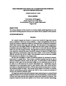
Figure 6: Flying ellipse where ~rk = (xk ; yk ) is the position of each panel's controlRpoint, j~rjk;j is the distance between two panels, and wk dsk is the source strength of the k'th panel. The source densities are determined by applying the boundary condition of zero normal ow through the body surface, i.e., @ = 0: (7) vn = @n k

This generates a system of linear equations A
w~ = ~b with each component of A given by 1 Z @ (ln r )ds ; Ak;j = k;j + (8) 2 2 @nk k;j j and the right hand side vector is simply bk = U0 sink , where k is the angle between the panel and the x-axis. 3. Panel Methods Once the vector of source densities is determined, the velocity eld may be obtained from the potential given Panel methods are eectively boundary element meth- in equation 6. Although the calculation of the inviscid ods for Computational Fluid Dynamics problems. ow eld past a body using the panel method consists These methods employ the surface of the body as the of several steps, we consider here only the numerically computational domain rather than the entire ow re- intensive solution procedure for the dense matrix equagion in which the body is immersed. This is not only tion A
w~ = ~b. computationally more ecient than a nite-dierence Consider rst the actions being performed upon the method, for example, but it also allows more complicated body shapes to be studied that otherwise may matrix and the right-hand side as part of the LU sonot be tractable if the ow domain is discretized by a lution procedure. The relative advantages and disadvantages of two possible arrangements, viz. (i) regular mesh. row distribution, and (ii) column distribution are disConsider gure 6 which shows panels around an el- cussed below. In the row distribution, the matrix rows lipse in a uniform incident velocity ow. Each k'th panel are distributed between processors either according to is centred around a control point at ~rk and has a source BLOCK or CYCLIC structures as seen in gure 7. The density wk . If the body is immersed in a uniform stream determination of the pivot requires a distributed global of velocity Uinf parallel to the x-axis, then the distri- test and the subsequent broadcast of the results. The bution of N source panels produces a potential given pivot row is then exchanged and broadcasted so that by8 it can be used in the elimination process. Note that if the rows are distributed in BLOCK structure, the Z N 1 X w ln j~rj ds ; (6) load-balance is poor since the elimination of the nal (~rk ) = U0 xk + 2 j j k;j rows involves only a subset of the available processors j =1 5 American Institute of Aeronautics and Astronautics

as indicated in gure 7. Despite reduced broadcast communication cost due to the reduction in the number of processors involved in the computation and the reduced computational load due to the shortening of the rows, there is still a signi cant load imbalance. This can be improved by using a CYCLIC distribution where alternate rows are on dierent processors. Here the computation is load-balanced until the number of rows remaining is less than the number of processors. A CYCLIC distribution also ensures that at each stage, the computation is load-balanced nely in contrast to the BLOCK distribution where each processor is expected to perform the elimination operation until the current row is part of the allocated set.

BLOCK

but also requires no communication. The row decomposition requires the broadcast of a partial matrix row in comparison to the broadcast of a multiplication factor in the column decomposition. The choice between these dierent structures may depend on the typical matrix size, number of processors and relative communication costs. The forward elimination stage of the solver in the Fortran 77 parent code is serial in nature as indicated in gure 9. Here the right-hand side is mapped according to the elimination stored within the lookup tables. The parallelism of the actual multiplication can be exploited, but this is a small fragment of the total work involved. The use of a distributed list also causes dif culties since the exchange of the entries in the righthand side subsequent to the pivoting operation in the matrix must be performed in order. Note that the ! forward elimination: nm = n -1 DO k=1,nm kp = k+1 l = jpvt(k) s = rhs(l) rhs(l) = rhs(k) rhs(k) = s DO i=kp,n rhs(i) = rhs(i) + a(i,k) * s ENDDO ENDDO

CYCLIC

Figure 7: Row distribution In the column distribution, the matrix columns are distributed as in gure 8. The global test to determine the pivot location is restricted to a single processor but the results must be broadcasted. The elimination process requires only the broadcast of a multiplying factor since all data for the elimination occur within columns. The same arguments regarding load-balancing and the relative merits of BLOCK and CYCLIC distributions apply here also and are illustrated in gure 8.

BLOCK

Figure 9: Use of list to sort RHS in forward elimination. inner loop over i can be expressed as a FORALL and is INDEPENDENT requiring a broadcast of the multiplication factor s. This, however, represents a very small and poorly load-balanced section of the algorithm. The back substitution phase can be considered equivalent to the factorization in gure 10; however, there is no pivoting since only one row can perform the required elimination. For all distributions, this section is poorly load-balanced and generates a low ratio of computation to communication. The degree of parallelism could be increased, but this would require writing complex code or explicit knowledge of the data decomposition that cannot be easily generalized. For both the forward elimination and back substitution, an alternative data distribuion could be considered. In gure 11, we show dierent possible data layouts for the back substitution phase. Note that a CYCLIC row distribution provides the best loadbalancing for both matrix and right-hand side vector operations. The column distributions are poorly load-

CYCLIC

Figure 8: Column distribution The dierence between row and column distributions can be summarized as follows. The row distribution features a distributed global test for the pivot, whereas, for column distribution, the global test is poorly balanced 6

American Institute of Aeronautics and Astronautics

Consider the prototype problem A~x = ~b to be solved for ~x which can be expressed in the form of iterative equations for the solution ~x and residual (gradient) ~r:

f90 code ! back substitution: do ka=1,nm km = n - ka k = km + 1 rhs(k) = rhs(k) / a(k,k) s = - rhs(k) do i=1,km rhs(i) = rhs(i) + a(i,k) * s enddo enddo rhs(1) = rhs(1) / a(1,1)

x~ k = ~xk?1 + k ~pk ~rk = ~rk?1 ? k ~qk

(9) (10)

where the new value of ~x is a function of its old value,  is the scalar step size, ~pk is the search direction vector at the k'th iteration, and ~qk = A~pk . The values of ~x are guaranteed to converge in, at most, n iterations, where n is the order of the system, unless the problem is ill-conditioned in which case roundo errors often prevent the algorithm from furnishing a suciently precise solution at the nth step. In well-conditioned problems, the number of iterations necessary for satisfactory convergence of the conjugate gradient method can be much less than the order of the system. Therefore, the iterative procedure is continued until the residual ~rk = ~bk ? A~xk meets some stopping criterion, typically of the form: k ~rk k 
(k A k
k ~xk k + k ~bk k), where k A k denotes some norm of A and  is a tolerance level. The CG algorithm uses

Figure 10: F90 code for back substitution. balanced since a single processor is required to work on the entire right-hand side vector of all stages of the back substitution. It is also possible to mix vector and matrix distributions; indeed, the cost of performing a REDISTRIBUTE on the matrix may be too high, but performing a REDISTRIBUTE on the right-hand side vector may accrue a communication saving. The low level of computation alongwith the global nature and small size of the messages to be exchanged suggest that this would be highly dependent on the problem size and features of the target architecture.

?
?
 = ~rk
~rk = p~k
A~pk ;

(11)

with the search directions chosen according to p~k = ~rk?1 + k?1 ~pk?1

(12)

with

k?1 = (~rk?1
~rk?1)=(~pk?2
A~pk?2) (13) which ensures that the search directions form an Aorthogonal system. The non-preconditioned CG algorithm is summarized as: p~ = ~r = ~b; ~x = 0; ~q = A~p  = ~r
~r;  = =(~p
~q ~x = ~x + ~p; ~r = ~r ? ~q DO k = 2, Niter 0 = ;  = ~r
~r; = =0 p~ = ~r + ~p; ~q = A
~p  = =~p
~q ~x = ~x + ~p; ~r = ~r ? ~q IF( stop criterion )exit ENDDO

Figure 11: Substitution inline with elimination

4. Conjugate Gradient Methods The classic Conjugate Gradient non-stationary iterative algorithm9 and references therein can be applied to solve symmetric positive-de nite matrix equations. They are preferred over simple Gaussian algorithms because of their faster convergence rate if the matrix A is very large and sparse.

for the initial \guessed" solution vector ~x0 = 0. Implementation of this algorithm requires storage for four vectors, viz. ~x, ~r, p~ and ~q as well as the matrix A and working scalars  and . Note that the work per iteration is modest, amounting to a single matrix-vector 7

American Institute of Aeronautics and Astronautics

product for A
~p, two inner products p~k
~qk and ~rk
~rk , trates how BLAS level library routines such as SAXPY and several simple ~x + ~y (SAXPY) operations, where and SDOT can be employed for a sparsely stored sys is scalar, and ~x and ~y are vectors. The number of tem. Each iteration of the CG algorithm in gure 13 multiplications and additions required for matrix-vector multiplication, inner products and SAXPY operations INTEGER row(nz), col(n+1) are O(n2 ), O(n), and O(n), respectively, for a vector of REAL A(nz), x(n), b(n), r(n), p(n), q(n) length n. REAL SDOT It is ecient in storage to represent an n  n dense DO i = 1, n matrix as an n  n Fortran array. However, if the max(i) = 0.0 trix is sparse, a majority of the matrix elements are zero r(i) = b(i) p(i) = b(i) and they need not be stored explicitly. It is therefore END DO customary to store only the nonzero entries and to keep rho = SDOT(n, r, r) track of their locations in the matrix. Special storage CALL SAYPX(p, r, beta, n) schemes not only save storage but also yield computaCALL MATVEC(n, A, row, col, p, q, nz) alpha = rho / SDOT(n, p, q) tional savings. Since the locations of the nonzero eleCALL SAXPY(x, p, alpha, n) ments in the matrix are known explicitly, unnecessary CALL SAXPY(r, q, -alpha, n) multiplications and additions with zero are avoided. A DO n = 2, Niter number of sparse storage schemes are known10 some rho0 = rho of which can exploit additional information about the rho = SDOT(n, r, r) sparsity structure of the matrix. We only consider here BETA = RHO / RHO0 the compressed row and compressed column schemes CALL SAYPX(p, r, beta, n) CALL MATVEC(n, A, row, col, p, q, nz) which can store any sparse matrix. ALPHA = RHO / SDOT(n, p, q) CALL SAXPY(x, p, alpha, n) CALL SAXPY(r, q, -alpha, n) IF( stop_criterion ) GOTO 300 END DO 300 CONTINUE

col :

row: 1

row:6

a11

a12

0

0

a15

0

a21

a22

0

a24

0

a26

a31

0

a33

0

0

0

0

a42

0

a44

0

0

a51

0

0

0

a55

0

0

a62

0

0

0

a66

Figure 13: Fortran 77 version of sparse storage CG (CSC format). performs three main computations: the vector-vector operations, inner product (here shown using BLAS routines) and the matrix-vector multiplication, shown explicitly in gure 14.

Sparse Matrix A col1

col2

col6

Compressed vector representation of A

q = 0.0 DO j = 1, n pj = p(j) DO 10 k = col(j) , col(j+1) - 1 q( row(k) ) = q( row(k) ) + A(k) * pj END DO END DO

Figure 12: Compressed Sparse Column(CSC) representation of sparse matrix A. The Compressed Sparse Column (CSC) storage scheme, shown in gure 12, uses the following three arrays to store an n  n sparse matrix with nz non-zero entries: (i) A(nz) containing the nonzero elements stored in the order of their columns from 1 to n, (ii) row(nz) that stores the row numbers of each nonzero element, and (iii) col(n+1) whose jth entry points to the rst entry of the j'th column in A and row. A related scheme is the Compressed Sparse Row (CSR) format, in which the roles of rows and columns are reversed. The serial Fortran 77 code fragment in gure 13 illus-

Figure 14: Sparse matrix-vector multiply in Fortran 77 (CSC format). In any parallel implementation that distributes the vectors and matrix A across processors' memories, the inner-products and sparse matrix vector multiplication require data communication. However, the data distributions can be arranged so that all of the other operations will be performed only on local data. 8

American Institute of Aeronautics and Astronautics

If all vectors are distributed identically among the processors, vector-vector operations such as SAXPY require no data communication in a parallel implementation since the vector elements with the same indices are involved in a given arithmetic operation and thus are locally available on each processor. Using P processors, each of these steps is performed in time O(n=P) on any architecture. A parallel implementation of the inner product (SDOT) with P processors, takes O(n=P) + ts
logP time on the hypercube architecture, where ts is the start-up time. If the reduction intrinsic functions are well supported by hardware reduction operations then the communication time for the inner-product calculations does not dominate. It now remains to discuss the multiplication of an n  n arbitrarily sparse matrix A with an n  1 vector p that gives another n  1 vector q. As in a dense matrix vector multiplication, each row of matrix A must be multiplied with the vector p. The computation and data communication costs vary depending on the distribution of the matrix A and vectors p and q. Here, we will describe two dierent data distribution schemes and show the associated costs of each. For the simplicity of the discussion, assume that the average number of nonzero elements per row in A is mz , and the total number of nonzero elements in the entire matrix is nz = mz  n. It may be desirable to control the number of non zero elements stored on each processor if there is some identi able structure to the sparse matrix. Generally this would require a data mapping that forces processors to perform the same number of scalar multiplications and additions while multiplying the matrix with a vector. This, however, requires that A(i; i) and p(i) are no longer necessarily assigned to the same processor, and thus requires communication before the multiplication. In the rst scheme, the sparse matrix A is partitioned row-wise among the processors in an even manner. The vectors p and q are aligned with the rows of the matrix A in all the processors. This distribution is shown in gure 15 and can be expressed in HPF as follows:

all-to-all broadcast of messages containing n=P vector elements among P processors, takes tstart?up
logP + tcomm
n=P time if a tree-like broadcasting mechanism is used. Here tstart?up is the start-up time, and tcomm is the transfer time per byte. In the second scheme, the matrix A is partitioned in a column-wise fashion amongst the processors such that each processor gets n=P columns. Vectors are partitioned amongst the processors uniformly. This corresponds to the following distribution directives in HPF: !HPF$ DISTRIBUTE A(*, BLOCK) !HPF$ DISTRIBUTE p(BLOCK) !HPF$ DISTRIBUTE q(BLOCK)

where only the distribution of the matrix itself is dierent from that for row-wise partitioning. As illustrated in gure 16, the vector p is already aligned with the rows of A, and hence performing the multiplication will not require any interprocessor communication. However, since each processor will have a partial product vector q at the end of the operation, these partial vectors should be merged into one nal vector. A global summation operation has to be performed with messages of size n=P where each processor sends its own portion of the partial vector to the owner of that portion according to the distribution directives given. This scheme is easily generalized to the CSC format. Procs Procs

0

1

2

3

Procs

0

0

1

1

1

2

2

3

3

Matrix A

!HPF$ DISTRIBUTE A(BLOCK, *) !HPF$ DISTRIBUTE p(BLOCK) !HPF$ DISTRIBUTE q(BLOCK)

Vector p

Vector q

Figure 15: Communication requirements of Matrix vector multiplication where A is distributed in a (BLOCK, *) fashion.

Since the nonzero elements are at random positions in A, a row can have a nonzero entry in any column. This requires the entire vector p to be accessible to each row so that any of its nonzero entries can be multiplied with the corresponding element of the vector. As the vector p is partitioned among the processors, this obligates an all-to-all broadcast of the local vector elements. This

In the computation phase, each processor performs an average of mz  n=P multiplications and additions if a sparse storage format is used. After the computation phase, each processor has the corresponding block of n=P elements of the resulting vector which is assigned 9

American Institute of Aeronautics and Astronautics

the loop. Such strategies have often been used successfully on vector machines although considerable care on the part of the programmer and signi cant reordering of the datasets are required. If, however, A is stored in CSR Format then the following HPF code fragment can be applied:

Procs Procs

0

1

2

3

Procs

0

1

2

3

0

1

(merge)

(merge)

(merge)

2

q = 0.0 FORALL( j = 1:n ) DO k = row(j), row(j+1)-1 q(j) = q(j) + a(k) * p( col(k) ) ENDDO ENDFORALL

3

(Merge of private copies)

Matrix A

Vector p

Vector q

Figure 16: Communication requirements of Matrix vector multiplication where A is distributed in a (*, BLOCK) fashion.

where the FORALL expresses parallelism across the jloop. This works because A(i; j) = A(j; i) for the case of CG where A must be symmetric. This works in row to that processor originally. Hence, no communication order, nishing up with one element of q at each iteration and the iterations are independent of one another. is needed to rearrange the distribution of the results. The HPF code for the CG algorithm for CSR format The communication time for column-wise partitioning is the same as the communication time for the global can be expressed as in gure 17. broadcast used in row-wise partitioning. It is not possible to reduce the communication time whether the REAL, dimension(1:nz) :: A matrix be partitioned into regular stripes either in a INTEGER, dimension(1:nz) :: col row-wise or column-wise fashion. INTEGER, dimension(1:n+1) :: row REAL, dimension(1:n) :: x, r, p, q It is important to note that this analysis assumes that the average number of non zero elements mz is represen- !HPF$ PROCESSORS :: PROCS(NP) !HPF$ DISTRIBUTE (BLOCK) :: q, p, r, x tative of all rows or columns. In practice, this is often !HPF$ A(BLOCK) not the case and individual rows or columns may have !HPF$ DISTRIBUTE DISTRIBUTE col(BLOCK) signi cant variations causing a load imbalance. The !HPF$ DISTRIBUTE row(CYCLIC((n+1)/np) data-parallel programming model, upon which HPF is (usual initialisation of variables) based, requires some well-de ned mapping of the data onto processors' memory to achieve a good computaDO k=1,Niter tional load balance and thus an ecient use of the parrho0 = rho rho = DOT_PRODUCT(r, r) ! sdot allel architecture. Clearly, this is not trivial for sparse beta = rho / rho0 storage schemes. p = beta * p + r ! saypx If the matrix A is stored in CSC format then the folq = 0.0 ! sparse mat-vect multiply lowing serial code fragment arises for the matrix-vector FORALL( j=1:n ) multiply (A
p~ = ~q): DO i = row(j), row(j+1)-1 q(j) = q(j) + A(i) * p(col(i)) END DO END FORALL

q = 0.0 DO j = 1, n pj = p(j) DO k = col(j), col(j+1)-1 q(row(k)) = q(row(k)) + a(k)*pj ENDDO ENDDO

alpha = rho / DOT_PRODUCT(p, q) x = x + alpha * p ! saxpy r = r - alpha * q ! saxpy IF ( stop_criterion ) EXIT END DO

In this case the use of indirect addressing on the write operation within the row summation of ~q causes the compiler to generate serial or sequential code. However, a directive could be used if it was known that there were no duplicate entries in any one segment of

Figure 17: HPF version of sparse storage CG (CSR format). A more extensive discussion of the Conjugate Gra10

American Institute of Aeronautics and Astronautics

dient method and High Performance Fortran may be found elsewhere11;12 . [2]

5. Conclusions

[3] We have illustrated some of the issues arising from the use of HPF for expressing algorithms in CFD applications. The advantages are the potential for faster computation on parallel and distributed computers, and additional code portability and ease of maintainence by comparison with message-passing implementations. [4] Disadvantages (in common with any parallel implementation) over serial implementations are additional temporary data-storage requirements of parallel algorithms. [5] The basic concepts of HPF have been demonstrated through examples which are characteristic of current scienti c and engineering codes. The removal of serial [6] features from sections of code has been as important as adding parallelism, and the relative merits of alternative decompositions have been compared. The actual choice between the dierent decompositions and the remapping of data between the dierent stages of the algorithm will, in general, depend upon the problem sizes being considered and the performance of the [7] TRANSPOSE intrinsic function (or the REDISTRIBUTE directive) for particular machines. Current HPF distribution directives only allow arrays to be distributed according to regular structures such as BLOCK and CYCLIC. Whilst this is adequate for dense or regularly structured problems, it does not [8] provide the necessary exibility for the ecient storage and manipulation of arbitrarily sparse matrices. [9] Finally, we repeat the general observation that implementations of numerically intensive applications on parallel architectures often encounter a tradeo between the most rapidly converging (in terms of numerical anal- [10] ysis) algorithm which do not parallelize well, and less numerically advanced algorithms which, because they can be parallelized, may produce the desired result in a faster absolute time. It is a pleasure to thank T.Haupt, K.Dincer and S.Ranka for [11] useful discussions regarding the work reported here.

References

[12]

[1] Cheng, Gang., Hawick, Kenneth A., Mortensen, Gerald, Fox, Georey C., \Distributed Computational Electromagnetics Systems", Proc. of the 7th

SIAM conference on Parallel Processing for Scienti c Computing, Feb. 15-17, 1995. High Performance Fortran Forum (HPFF), \High Performance Fortran Language Speci cation," Scienti c Programming, vol.2 no.1, July 1993. Bozkus, Z., Choudhary, A., Fox, G., Haupt, T., and Ranka, S., \Fortran 90D/HPF compiler for distributed-memory MIMD computers: design, implementation, and performance results," Proceedings of Supercomputing '93, Portland, OR, 1993, p.351. Metcalf, M., Reid, J., \Fortran 90 Explained", Oxford, 1990. Koelbel, C.H., Loveman, D.B., Schreiber, R.S., Steele, G.L., Zosel, M.E., \The High Performance Fortran Handbook", MIT Press 1994. Bogucz, E.A., Fox, G.C., Haupt, T., Hawick, K.A., Ranka, S., \Preliminary Evaluation of HighPerformance Fortran as a Language for Computational Fluid Dynamics," Paper AIAA-94-2262 presented at 25th AIAA Fluid Dynamics Conference, Colorado Springs, CO, 20-23 June 1994. Hawick, K.A., and Wallace, D.J., \High Performance Computing for Numerical Applications", Keynote address, Proceedings of Workshop on Computational Mechanics in UK, Association for Computational Mechanics in Engineering, Swansea, January 1993. Fletcher, C. A. J., \Computation Techniques for Fluid Dynamics", Vol. II, Springer-Verlag, 1991. Dongarra, J.J., Du, I.S., Sorensen, D.C., van der Vorst, H.A., \Solving Linear Systems on Vector and Shared Memory Computers", , SIAM, 1991. Barrett, R., Berry, M., Chan, T.F., Demmel, J., Donato,. J., Dongarra, J.J., Eijkhout, V., Pozo, R., Romine, C., van der Vorst, H.A. \Templates for the Solution of Linear Systems: Building Blocks for Iterative Methods", SIAM, 1994. Hawick, K. A., Dincer, K., Robinson, G. and Fox, G. C., \Conjugate Gradient Algorithms in Fortran 90 and High Performance Fortran", Northeast Parallel Architectures Center Report No. SCCS-691, Syracuse University, 1995. Dincer, K., Hawick, K. A., Choudhary, A. and Fox, G. C., \High Performance Fortran and Possible Extensions to Support Conjugate Gradient Algorithms", Northeast Parallel Architectures Center Report No. SCCS-703, Syracuse University, 1995.

11 American Institute of Aeronautics and Astronautics