P1.17
CFD INVESTIGATION OF AIRFLOW AROUND A SIMPLE OBSTACLE WITH SINGLE HEATING WALL 1
1.
R. Dimitrova1*, J.-F. Sini1, K. Richards2, M. Schatzmann2 Laboratoire de Mécanique des Fluides, Ecole Centrale de Nantes, France 2 Meteorological Institute, University of Hamburg, Germany
INTRODUCTION
Established within the framework of the European Commission Training and Mobility of Researchers Programme (TMR) the primary objective of the ATREUS project (http://aix.meng.auth.gr/atreus/) is to bring together current knowledge on parameters determining the microclimatic environment of urban areas and to further expand and use this knowledge in the optimization of heating and ventilation of buildings. Numerical studies into the characteristics of wind fields in street canyons and the influence of the urban heat islands on urban climates are numerous: Herbert and Herbert (2002), Xia and Leung (2001), Johnson and Hunter (1998, 1999), Ca et al. (1995), Sakakibra (1996), Hunter et al. (1992). But there are few numerical studies that investigate the direct influences of surface heating on the flow regime within a street canyon: Ca et al. (1995), Mestayer et al. (1995), Sini et al. (1996), Kim and Baik (1999, 2001). In general these investigations showed the degree of flow modification to be dependent primarily on the surface being heating i.e. windward, leeward (with respect to the ambient wind direction) or ground heating, and the aspect ratio W/H, where W is the street width and H is the height of the building. There are essentially only three wind tunnel studies that look at the influence of thermal effects within the vicinity of buildings: Kovar-Panskus et al. (2001), Uehara et al. (2000), Ruck (1993). Of these only Kovar-Panskus et al. (2001) investigate the influence of thermal effects within a simplified street canyon. Cermak (1996) gives examples of physical modelling using boundary layer wind tunnels and convection chambers to model steady state thermal effects on flow and dispersion over various urban terrains but again only considers the more global effects not local effects within a single street canyon. There have been many field studies conducted to understand more about urban microclimates and how the localized climate within a street canyon may be influenced by human activity and atmospheric conditions, for example Nunez and Oke (1977), Yoshida et al. (1990/91), Eliasson (1996), Pearlmuter et al. (1999), Santamouris et al. (2001). However fewer studies look more specifically at the influence of localized surface heating due to solar radiation on incanyon flow fields: Nakamura and Oke (1988), Santamouris et al. (1999), Vachon et al.(2000). ___________________________________________ * Dimitrova Reneta, Ecole Centrale de Nantes, Laboratoire de Mécanique des Fluides, 1, rue de la Noe – BP 92101, 44321 Nantes Cedex 03, France; e-mail :
[email protected]
However knowledge on thermal effects due to direct solar radiation within the vicinity of buildings is limited with only a handful of experimental, field and numerical studies show varying degrees of influence of thermal effects (Nakamura and Oke, 1988; Ruck, 1993; Mestayer et al, 1995; Sini et al, 1996; Kim and Baik, 1999; Santamouris, 1999; Uehera et al, 2000; Louka et al, 2001; Kovar-Panskus et al., 2001; Huizhi et al, 2003; Xie et al, 2005). A combined numerical-field study of Louka et al. (2001) using the Computation Fluid Dynamics (CFD) code CHENSI within TRAPOS project reported the numerical model overestimates the thermal effects on the canyon airflow, predicting two counter-rotating vortices when only one recirculation vortex was observed in the field. Model-scale wind tunnel investigations show further inconsistency with the numerical predictions but are in themselves limited in their scope of study to either for 2D cavities and or full-heated cylindrical building with square crosssection. The aim of the current work is to provide information to enhance the understanding of the flow phenomena and flow perturbations due to wall heating within the vicinity of a building. The heating and cooling requirements of buildings are strongly associated with the micro-climatic conditions that develop within their vicinity, in particular influences due to direct solar radiation. The efficiency of wall mounted air conditioning (A/C) systems maybe severely compromised by an increase in local air temperature. It is therefore important to understand the thermal convection around a building and its influence on local air patterns in order that the efficiency of air-conditioning systems maybe comprehensively assessed. There is insufficient reliable field and experimental data for comprehensive numerical model validation. The following paper describes a validation study in which the thermal effects within the vicinity of a single block building with leeward wall heating has been modelled physically and reproduced numerically in a micro-scale model. A three-dimensional numerical simulation (using CFD code CHENSI) of airflow around simple obstacle with vertical wall heating is presented in this study. The two turbulence models, the standard k-ε model and Chen&Kim (1987), are employed to predict the flow field and thermal effects. Different ratios of buoyancy to inertia forces have been applied to investigate perturbations on the flow due to thermal effects. Model’s results were improved by optimisation of the inflow boundary conditions.
2.
MODELLING APPROACH
A 1:100 scale single block building (a cube) has been built and set-up in the Stratified Boundary Layer Wind Tunnel at the Meteorology Institute of Hamburg University. This physical model is unique in that only one of its vertical faces is heated (the leeward face) in order to simulate the influence of solar radiation on one wall of an isolated building. The cube is made from plaster of Paris with the heated face comprising an aluminum plate, which is heated from the inside. Figure 1 shows the model and set-up in the wind tunnel.
Wind direction
with the official German guideline VDI 3783/Part 12 the modelled boundary layer flow demonstrates the behaviour and characteristics of an urban/inner city like roughness (to a scale of 1:100) with a power law exponent α=0.52, roughness length zo=2.9m and constant shear layer to 50m. The CFD code CHENSI (Sini et al, 1996) solves unsteady incompressible RANS equations with the Boussinesq approximation and different k-ε turbulence closure models. The code employs a finite difference method with an upwind weighted scheme for advection. The code is used for simulations of flow, heat transfer and passive scalar dispersion on a hexahedral stretched grid. The time scheme is explicit and first order accurate. Wall functions were used at the solid boundaries. Care was taken to ensure that the physical model was reproduced in the numerical model. The inflow boundary is defined at 4H upstream of the model as was defined in the wind tunnel. The mesh used for the numerical calculations has total number of 221340 cells (Figure 2). y/H
4
a
3 2
Leeward heated face
Figure 1 – Physical model set-up (the cube is outlined in white for clarity) While using a single block building may seem a somewhat simplistic approach and perhaps in someway unrealistic, the essence of simplicity is vital when producing data for the validation of a numerical model. The influence of thermal effects with respect to the mechanical flow around the building is modelled using the ratio of Grashof number to the square of 2
Reynolds number (Gr/Re )
βgH∆T
1 0 -1 -2 -3 -4 -4 5
2 U H where β is
0
1
2
3
4
5
6
z/H
7 b
2 1
U H is wind velocity at H just upstream of the model.
Reynolds number independence of the flow field around the model has been assured for these low wind speed conditions (Uref=1m/s). An arrangement of sharp edged roughness elements and upstream vortex generators are used to simulate a turbulent atmospheric boundary layer approach flow (Figure 1). The aerodynamic properties of the approach flow were measured using a 2D fibre-optic Laser Doppler Anemometer (BSA-LDA, Dantec ®). In accordance
-1
3
temperature Tw and ambient temperature Tref and
temperature Tw in order to avoid technical difficulties.
-2
4
the coefficient of thermal expansion, g acceleration due to gravity, H is the model height, ∆T is the temperature difference, between the mean wall
Low wind speed conditions are used in order to get maximum thermal effects keeping limited wall
x/H
-3
0 -4
x/H
-3
-2
-1
0
1
2
3
4
5
6
Figure 2. Computational mesh - horizontal (a) and vertical (b) section 3.
SIMULATION AND ANALYSIS
3.1 “Cold cube” case The so named “cold cube” case was used to validate the numerical model. The 3D flow field around the cold cube was measured using BSA-LDA. In addition to the mean longitudinal, lateral and
7
3
3
x/H=-0,625
2
x/H=0,625
z/H
z/H
1
1 2 3
1 2 3
0
0 0
0,02 0,04 0,06 0,08
k/Uref
2
0,1
0
0,02 0,04 0,06 0,08
k/Uref
2
2
x=-0,625
1
y/H
1
0
0
-1
-1
1 2 3
1 2 3 -2
-2 -0,2
x=0,75
0
0,2
0,4
u /Uref
0,6
0,8
-0,2
0
0,2
0,4
0,6
0,8
u /Uref
Figure 4. Comparison of the horizontal plots for u velocity component observed in the wind tunnel with predictions at x/H=-0.625 and x/H=0.75 at y/H=0 (- denotes upstream the cube centre). Numbers correspond to: 1 - Case 1; 2 - Case 2; 3 – experimental data. The model was able to reproduce well the general flow pattern observed within wind tunnel (Figure 5). The oncoming flow exhibits an impingement region at the windward side of the obstacle. When approaching the cube the flow separates due to increasing pressure leading to the development of a main horseshoe vortex wrapping around the cube. At the upper leeward edge of the
2
1
Using the same inflow conditions comparisons between these models with experimental data, for different locations, have been made in order to choose the better turbulent model. The locations with the biggest disagreement with the experimental data are shown only (Figure 3). CHENSI tends to overproduce turbulent kinetic energy in the impingement region (at x/H=-0.625). Both models give reasonable results in the cavity zone. The Chen&Kim model gives better results with less disagreement with experimental data. Comparison between Case 1 and Case 2 with wind tunnel data have been made using Chen&Kim turbulent model. The difference between these cases is negligible at the centre cube plane, but are observed far from the obstacle on the horizontal plots for u velocity component. The locations close to the obstacle are shown only (Figure 4). Introducing the non-uniform inflow improves the numerical results.
y/H
vertical wind velocity components u , v and w respectively, the RMS values of each velocity component as well as the Reynolds shear stresses u′w′ and u ′v ′ were also recorded. At the upwind free boundary an inlet velocity profile for the atmospheric boundary layer was applied. Numerical data for two different cases were produced using uniform (Case 1) and non-uniform (Case 2) inflow fields in the horizontal plane. This was done in order to achieve the flow in-homogeneity observed in the experimental data. For Case 1 a inlet velocity profile was constructed using a power law with parameters provided by wind tunnel experiment and a vertical profile for turbulent kinetic energy constructed based on measured data at the cube centre plane only. For Case 2 a linear interpolation was made between available experimental data in different locations in the horizontal plane (y/H=-1.5; 0; 1.5). Two turbulence models were employed to predict the flow field for Case 1. The turbulent kinetic energy k and its dissipation rate ε are calculated from the semi-empirical transport equations of Hanjalic and Launder (1972) and the empirical modelling constants are assigned the most commonly used values for industrial flows as in Launder and Spalding (1974) for the standard k-ε model. The inconsistency of this model is very often attributed to the dissipation rate equation, which is highly empirical in nature. Improvement of the model performance is usually achieved by modifying this equation. In the paper of Chen and Kim (1987) the general approach is taken by adding a second time scale of the production range of turbulent kinetic energy spectrum to the dissipation rate equation. This extra time scale enables the energy transfer mechanism of the turbulence model to respond to the mean strain more effectively. One extra term along with one extra modelling constant added to the standard k-ε model.
0,1
2
Figure 3. Comparison of the profile of the turbulent kinetic energy observed in the wind tunnel with predictions at x/H=-0.625 and x/H=0.625 at y/H=0 (- denotes upstream the cube centre). Numbers correspond to: 1 - standard k-ε model; 2 - Chen&Kim model; 3 – experimental data
Numerical results for Case 2 are shown at the cube centre plane. The agreement between measured and computed data at the centre plane close to the obstacle is excellent for the velocity field (Figure 6) but not so good for turbulent kinetic energy (Figure 7). Table 1 summarizes the characteristic lengths of the flow field around the cube as predicted by numerical code and derived from the measurements. Table 1. Characteristic lengths of the flow field Figure 5. Vertical cross section of the dimensionless u component normalized with the free-stream velocity (Uref=1m/s) obstacle the flow separates again and leads to an extended lee vortex formed in the cavity zone immediately behind the cube which interacts with the horseshoe vortex. 3
3
x/H=-0,625
2
x/H=0,625
Characteristic lengths:
Numerical produced
Experimental measured
Stagnation point Zs/H Reattachment point XR/H
0.29 2.0
0.18 1.34
CHENSI predicts a higher value for the stagnation point height on the upwind edge. Close to the observed reattachment point at the centre plane, the model computes a negative velocity close to the surface indicating that this position is predicted to be still far inside the cavity zone. CHENSI overestimates the recirculation length by about 30%.
2
z/H
z/H
3.2 “Heated cube” case
1
1
1 2
1 2 0
0 -0,2
0
0,2
0,4
0,6
0,8
-0,2
1
u /Uref
0
0,2
0,4
0,6
0,8
1
u /Uref
the relation Gr/Re2 as opposed to
Figure 6. Comparison of the profile of the u velocity component observed in the wind tunnel with predictions at x/H=-0.625 and x/H=0.625 at y/H=0 (- denotes upstream the cube centre). Numbers correspond to: 1 – model data; 2 – experimental data. 3
3
x/H=0,625
x/H=-0,625
2
z/H
z/H
2
1
1
1
1
2
2 0
0 0
0,02 0,04 0,06 0,08
k/Uref
2
0,1
0
0,02 0,04 0,06 0,08
k/Uref
2 When the relation Gr/Re ≈1 motion is induced by 2 both thermal and mechanical effects and if Gr/Re >1 then thermal effects are dominant. Different values of Gr/Re2 have been selected in order that the influence of these thermal effects may be assessed. For practical reasons the parameter ∆T is used to govern
0,1
2
Figure 7. Comparison of the profile of the turbulent kinetic energy observed in the wind tunnel with predictions at x/H=-0.625 and x/H=0.625 at y/H=0 (- denotes upstream the cube centre). Numbers correspond to: 1 – model data; 2 – experimental data.
U H . With
reference to Figure 1, the leeward face is heated from the inside by a radiant heater to a known mean wall temperature surface
Tw , monitored and recorded using
mounted
thermocouples.
The
ambient
temperature Tref is monitored and recorded using a column of 30 semi-conductor temperature transducers that measure the mean temperature over the height of the wind tunnel test section. An array of up to 20 thermocouples measures the mean temperature field around and in the wake of the model building. It was impossible to completely isolate the heated face from the rest of the model therefore further surface mounted thermocouples on the sides and roof of the cube record mean temperature and thus allow any heat loss to be accounted for. As in the “cold cube” case the 3D velocity field will be measured using BSA-LDA. Simulations were performed considering the 2 thermal conditions Gr/Re ≈ 1 and 1.5. Figure 8 shows contour plots of velocity field with wall heating for both cases. The thermally induced upward motion close to the heated face acts together with the mechanical flow to strengthen the clockwise rotating vortex within the wake of the cube. While this is observed for both
a
z/H
1 m/s
2
1.5
1 0 0
0.5 0
0 0
0 -1.5
-1
-0.5
0
0.5
1
1.5
2
1
0
0
0
2.5 x/H
1 m/s U 0.7 0.65 0.6 0.5 0.4 0.3 0.2 0.1 0.05 0 -0.05 -0.1 -0.15
1.5
1 0 0
0.5 0
0
0
0 -1.5
-1
-0.5
0
0.5
1
1.5
2
cases the effect is stronger for Gr/Re2 ≈ 1.5 as buoyancy forces become more significant. Compared with the “cold cube” case the recirculation length for 2 the condition Gr/Re ≈ 1.5 is approximately 10% shorter (XR/H=1.8 as opposed to 2.0) but the size of the region has expanded due to the added buoyancy and the increase in vertical motion. Figure 9 shows contour plots of vertical velocity field with and without wall heating. In both thermal cases there is the tendency for an increase in the magnitude of the vertical velocity and an extension of the cavity zone through increased upward motion (Figure 9b, c). The tendency is more stronger for 2 thermal conditions Gr/Re ≈ 1.5. The dynamics and thermal buoyancy act in concert: compared to the isothermal flow, the intensity of the unique vortex is increased, generating a net increase in the vertical exchanges and exchange rates. The wall heating can largely influence the flow pattern due to vertical transport capabilities. 1m/s
2
1
0
0
0
1
a W 0.2 0.15 0.1 0.08 0.06 0.05 0.04 0.03 0.02 0.01 0 -0.001 -0.01 -0.05 -0.1
0
2
x/H
0
1
2
z/H
y/H=0 0 0
0
1
0
0
1
2
z/H
y/H=0.5
1
0
0
0
0
0
1
2
c W 0.2 0.15 0.1 0.08 0.06 0.05 0.04 0.03 0.02 0.01 0 -0.001 -0.01 -0.05 -0.1
x/H 1m/s
2
W 0.2 0.15 0.1 0.08 0.06 0.05 0.04 0.03 0.02 0.01 0 -0.001 -0.01 -0.05 -0.1
x/H
1m/s
2
2.5 x/H
Figure 8. Vectors and contours for u velocity 2 component for “heated cube” with values Gr/Re ≈ 1 2 (a) and Gr/Re ≈ 1.5 (b).
z/H
0
0
2
b
1m/s
b
z/H
0
z/H
2
U 0.7 0.65 0.6 0.5 0.4 0.3 0.2 0.1 0.05 0 -0.05 -0.1 -0.15
d W 0.2 0.15 0.1 0.08 0.06 0.05 0.04 0.03 0.02 0.01 0 -0.001 -0.01 -0.05 -0.1
x/H
Figure 9. Contours for vertical velocity and velocity vectors for “cold cube” (a); “heated cube” with values 2 2 Gr/Re ≈ 1 (b) and Gr/Re ≈ 1.5 (c) at cube centre 2 plane y/H=0; “heated cube” with value Gr/Re ≈ 1.5 at y/H=0.5 (d). The vertical velocity pattern is different in the planes of cube’s lateral faces, where the buoyancy effect is stronger compared with the cube centre plane (Figure 9c, d). Vertical velocity plots for isothermal and both thermal cases are shown at the cube centre plane at different levels (Figure 10). The magnitude of the 2 vertical velocity increases by about 85% (Gr/Re ≈ 2 1.5) and 48% (Gr/Re ≈ 1) near the wall (x/H=0.1) compared with “cold cube” case. The maximum values in the vertical velocity field occur at z/H=0.75
and the minimum at about x/H=0.4 from the wall for both thermal cases. The most important feature is the development of a steep horizontal gradient very close to the wall. The vertical velocity changes sign for both thermal cases compared with “cold cube” case at distance more than x/H=1. 0,15
0,15
z/H=0.5
0,1
y/H
c
2
W 0.2 0.18 0.16 0.15 0.14 0.12 0.1 0.05 0.04 0.03 0.02 0.01 0 -0.01 -0.02 -0.03 -0.04 -0.05 -0.1
1
0
z/H=0.75
0,1 w [m/s]
w [m/s]
-1 0,05
0,05
0
-2 -1
0
1 2 3
1 2 3
-0,05
-0,05 0
0,5
x/H
1
1,5
0
0,5
x/H
1
1,5
Figure 10. Vertical velocity plots at different levels at cube centre plane (y/H=0). Numbers correspond to: “cold cube” (1), “heated cube” with value Gr/Re2 ≈ 1 2 (2) and Gr/Re ≈ 1.5 (3). The horizontal plots of the vertical velocity field at level z/H=0.75 where maximum values achieved and are shown in Figure 11. Additional circulation due to thermal effects appears close to the lateral cube faces on the contrary to strong upward motion near to the lateral cube’s edges. Two mechanically induced vortices with opposite rotation move the heated air y/H
W 0.2 0.18 0.16 0.15 0.14 0.12 0.1 0.05 0.04 0.03 0.02 0.01 0 -0.01 -0.02 -0.03 -0.04 -0.05 -0.1
1
0
-1
0
1
2
3
2
3
4 x/H
Figure 11. Horizontal plots of vertical velocity field for 2 “cold cube” (a) and “heated cube” with values Gr/Re 2 ≈ 1 (b) and Gr/Re ≈ 1.5 (c) near the lateral cube’s faces and contribute to the upward motion. Downward motion with the same magnitude similar to that upstream of the cube can be 2 seen for case Gr/Re ≈ 1.5. The structure of the temperature field is presented at Figure 12. The maximum difference between wall and ambient temperatures appears near the top outer edges of the cube. z/H
TP a 70 60 50 45 40 35 30 25 20 18 16 14 12 10 8 6 5 4 3 2 1
1m/s
2
1
0
0
1
z/H
2
b
2
W 0.2 0.18 0.16 0.15 0.14 0.12 0.1 0.05 0.04 0.03 0.02 0.01 0 -0.01 -0.02 -0.03 -0.04 -0.05 -0.1
1
0
-1
0
1
2
3
4 x/H
1
0
0
1
x/H TP b 70 60 50 45 40 35 30 25 20 18 16 14 12 10 8 6 5 4 3 2 1
1m/s
2
4 x/H
y/H
-2 -1
1
a
2
-2 -1
0
2
x/H
Figure 12. Velocity vectors and contours for temperature difference between wall and ambient air different “heated cube” cases with values Gr/Re2 ≈ 1 2 (a) and Gr/Re ≈ 1.5 at central cube plane y/H=0.
Unfortunately at the time of writing this paper the experimental work was still in progress therefore no validation can be performed. 4.
CONCLUSIONS
A wind tunnel study of the thermal effects within the vicinity of single block building with leeward wall heating is being conducted to provide validation data for a numerical micro-scale model. To model such thermal influences at scale is difficult. But with certain physical and theoretical compromises a physical wind tunnel model has been developed which can simulate different thermal conditions with respect to the ratio 2 Gr/Re thus providing data for validation. The CHENSI model predicted adequately the general flow features and showed good agreement with the experimental data for “cold cube” case. The influence of the thermal 2 effects were significant for case Gr/Re ≈ 1.5. The recirculation length was reduced by approximately 10% compared to the “cold cube” case. So far the thermal predictions have shown some modification to the isothermal flow field, with a general strengthening in the flow particularly close to the leeward heated wall. However one must be cautious at this stage to make any definitive conclusions without the verification from wind tunnel data. 5.
ACKNOWLEDGEMENTS
The present work was carried out within the ATREUS network (Advanced Tools for Rational Energy Use towards Sustainability with emphasis on microclimatic issues in urban applications) in the framework of the European Community Marie Curie Research Training Programme. The numerical calculations were carried out on the supercomputers of the CNRS national computing centre. Complete computer support was given by the Scientific Council of Institut de Développement et de Recherche pour l’Informatique Scientifique (IDRIS), Orsay, France. 6.
.REFERENCES
Ca, V. T., Asaeda, T. Ito, M. and Armfield, S., 1995: Characteristics of wind field in a street canyon. Journal of Wind Eng. Ind. Aerodyn., 57(1), 63-80. Cermak., J. E., 1995: Thermal effects on flow and dispersion over urban areas: capabilities for prediction by physical modeling. Atmos. Env., 30(3), 393-401. Chen, Y. and Kim S., 1987: Computation of turbulent flows using an extended k-ε turbulence closure model. Report NASA-CR-179204. Eliasson, I., 1996: Urban nocturnal temperatures, street geometry and landuse. Atmos. Env., 30(3), 379392. Hanjàlic, R. and Launder B. E., 1972: A Reynolds stress model of turbulence and its application to thin
shear flows. J. Fluid Mech., 52, 609-638. Herbert, J. M. and Herbert R. D., 2002: Simulation of the effects of canyon geometry on thermal climate in city canyons. Mathematics and Computers in Simulation, 59(1-3), 243-253. Huizhi, L., Bin, L., Fengrong, Z., Boyin, Z. and Jianguo, S., 2003: A laboratory model for the flow in Advances in Atmospheric Sciences. 20, NO.4, 554564. Hunter, L. J., Johnson, G. T. and Watson, I. D. 1992: An investigation of three-dimensional characteristic of flow regimes within the urban canyon. Atmos. Env., 26B, 425-432. Johnson, G. T. and Hunter, L. J., 1998: Some insights into typical urban canyon airflows. Atmos. Env., 33(24-25), 3991-3999. Johnson, G. T. and Hunter, L. J., 1999: Urban wind flow: wind tunnel and numerical simulations – a preliminary comparison. Environmental Modelling and Software, 13(3-4), 279-286. Kim, J-J. and Baik, J-J., 1999: A numerical study of thermal effects on flow and pollutant dispersion in urban street canyons. J. App. Meteor., 38(9), 12491260. Kim, J-J. and Baik, J-J., 2001: Urban street-canyon flows with bottom heating. Atmos. Env., 35(20), 33953404. Kovar-Panskus, A., Moulinneuf, L., Robins, A., Savory, E. and Toy, N., 2001: The influence of solarinduced wall heating on the flow regime within urban rd street canyons. 3 International Conference on Urban Air Quality, 19-23rd March, Loutraki, Greece. Launder B. E. and Spalding D. B., 1974: The numerical computation of turbulent flows. Comput. Meth. Appl. Mech. Engng., 3, 269-289. Louka, P., Vachon, G., Sini, J-F., Mestayer, P. G. and Rosant, J-M., 2001: Thermal effects on the airflow in a street canyon – Nantes ’99 experimental results and model simulations. Water, Air, and Soil Pollution, Focus 2, 351–364. Mestayer, P. G., Sini, J-F. and Jobert, M., 1995: Simulation of wall temperature influence on flow and rd dispersion within street canyons. 3 International Conference on Air Pollution, Proto Carras, Greece Vol. 1; Turbulence and Diffusion, 109-116. Nakamura, Y. and Oke, T.R., 1988: Wind, temperature and stability conditions in an east-west oriented urban canyon. Atmos. Env., 22(12), 26912700.
Nunez, M. and Oke, T. R., 1977: Energy-balance of an urban canopy. J. Appl. Meteor., 16(1), 11-19. Pearlmutter, D., Bitan, A. and Berliner, P., 1999: Microclimatic analysis of “compact” urban canyons in an arid zone. Atmos. Env., 33(24-25), 4143-4150. Ruck, B., 1993: Wind-tunnel measurements of flow field characteristics around a heated model building. Journal of Wind Engineering and Industrial Aerodynamics, 50(1-3), 139-152. Sakakibara, Y., 1996: A numerical study of the effect of urban geometry upon surface energy budget. Atmos. Env., 30(3), 487-496. Santamouris, M., Papanikolaou, N., Koronakis, I., Livada, I., and Assimakopoulos, D. N., 1999: Thermal and airflow characteristics in a deep pedestrian canyon under hot weather conditions. Atmos. Env., 33(27), 4503-4521. Santamouris, M., Papanikolaou, N., Livada, I., Koronakis, I., Georgakis, C., Argiriou, A. and Assimakopoulos, D. N., 2001: On the impact of urban climate on the energy consumption of buildings. Solar Energy, 70(3), 201-216. Sini, J-F., Anquetin, S., and Mestayer, P. G., 1996: Pollutant dispersion and thermal effects in urban street canyons, Atmos. Env., 30(15), 2659-2677.
Uehara, K., Murakami, S., Oikawa, S. and Wakamatsu, S., 2000: Wind tunnel experiments on how thermal affects flow in and above urban street canyons. Atmos. Env., 34(10), 1553-1562. Vachon, G., Rosant, J-M., Mestayer, P. G., Louka, P. and Sini, J-F., 2000: Pollutant dispersal in an urban street canyon in Nantes: experimental study. th st EUROTRAC-2 Symposium 2000, 27 – 31 March 2000, Garmisch-Partenkirchen, Germany VDI-guideline 3783/Part 12, 2000: Physical Modelling of Flow and Dispersion Processes in the Atmospheric Boundary Layer – Application of wind tunnels. Beuth Verlag, Berlin 2000. Xia, J. Y. and Leung, D.Y.C., 2001: Numerical study on flow over buildings in street canyon. Journal of Environmental Engineering-ASCE, 127(4), 369-376. Xie, X., Huang, Z.,, S., Wang, J. and Xie, Z., 2005: The impact of solar radiation and street layout on pollutant dispersion in street canyon. Building and Environment, 40, 201-212. Yoshida, A., Tominaga, K. and Watatani, S., 1990/91: Field measurements on energy balance of an urban canyon in the summer season. Energy and Buildings, 15(3-4), 417-423.