cfd modeling of chemical reactors: single-phase complex ... - CiteSeerX

European Conference on Computational Fluid Dynamics ECCOMAS CFD 2006 P. Wesseling, E. O˜ nate and J. P´ eriaux (Eds) c TU Delft, The Netherlands, 2006

CFD MODELING OF CHEMICAL REACTORS: SINGLE-PHASE COMPLEX REACTIONS AND FINE-PARTICLE PRODUCTION Ying Liu∗, Qing Tang† and Rodney O. Fox∗ ∗ Department

of Chemical and Biological Engineering, Iowa State University Ames, IA 50010-2230, U.S.A. e-mail: [email protected], [email protected] † Reaction Engineering International Salt Lake City, UT 84101, U.S.A. e-mail: [email protected]

Key words: Computational Fluid Dynamics, Chemical Reactors, Turbulent Reacting Flow, Quadrature Method of Moments Abstract. Computational fluid dynamics (CFD) is a useful tool for modeling chemical reactors. However, because the design goals and expected outcomes are different than in “traditional” CFD applications, chemical reactors require special attention to the treatment of chemical reactions, and heat and mass transfer. Here we provide an overview of the modeling components needed to describe single-phase reactors with complex reactions and possible fine-particle production, and show some successful examples from our laboratory. The models are described in the context of the Reynolds-average transport equations, but can be easily modified for use with large-eddy simulations. The examples range in complexity from turbulent mixing of a single scalar to turbulent reacting flow with the formation of fine particles. For the latter, we illustrate how the number density function describing the particle population can be efficiently integrated with a CFD code by using the quadrature method of moments.

1

INTRODUCTION

Computational fluid dynamics (CFD) is most often associated with solving for the fluid dynamics in single and multiphase flows. While this is certainly a critical part of modeling chemical reactors, it is only the starting point. When developing CFD models for chemical reactors much of the effort is directed at correctly describing the chemical and physical processes that influence the productivity of the reactor. For example, chemical reactions and heat and mass transfer must be accurately modeled in order to predict the selectivity and yield of mixing-sensitive reactions. Depending on the reactor type (single vs. multiphase, gas vs. liquid, etc.), the rate-controlling steps that must be included in 1

Ying Liu, Qing Tang, and Rodney O. Fox

the CFD model can be very different. Thus, unlike in more “traditional” applications of CFD, this makes CFD modeling of chemical reactors more challenging (and perhaps more interesting) for the engineers responsible for developing the model. In this work we discuss CFD modeling of single-phase chemical reactors under turbulent flow conditions, which includes reactors for making fine particles. For such reactors, there are several key components in the CFD model that influence the accuracy of the predictions: • The turbulence model that is used to describe the fluid dynamics. • The scalar transport model that is used to describe turbulent mixing. • The model used to describe the effect of turbulence on chemical reactions, and vice versa. • The transport model used to describe the evolution of fine particles due to nucleation, growth, aggregation, etc. As we will see in the following discussion, each of these modeling components can be added sequentially to arrive at the overall CFD model. Likewise, each of them can (and should) be validated experimentally with appropriate measurements (i.e. the turbulence statistics should be measured directly and not inferred indirectly from, for example, measurements of product yield.) Likewise, because the chemical kinetics and particle evolution processes will have a strong influence on the CFD predictions, it will be important that models for these processes be adequately tested in simplified flow configurations before they are used in CFD models of plant-scale chemical reactors. The remainder of this work is arranged as follows. First we discuss CFD models for turbulent mixing and show how such models can be validated with experiments. Next we add a micromixing model for mixing-sensitive reactions and apply it to a liquid-phase confined impinging-jets reactor to illustrate how CFD can be used to understand mixing in such devices. In the third example, we consider turbulent combustion wherein the chemical reactions affect the flow field through the density field. Finally, in the last example we show how the number density function needed to describe a population of fine particles can be included in CFD models for chemical reactors. All of the examples use models developed at Iowa State, but we should point out that there are many other examples in the literature that could also be cited. Our goal here is not to give an exhaustive overview, but rather to illustrate the necessary steps and concepts required to develop an accurate CFD model. 2

TURBULENT MIXING

Most chemical reactors are designed to operate in the turbulent regime to maximize throughput. It follows that a detailed understanding of turbulent mixing is crucial for proper design and optimization of chemical reactors, inspiring numerous experimental 2

Ying Liu, Qing Tang, and Rodney O. Fox

and computational studies on turbulent mixing over the years 1,2,3. In addition to describing large-scale segregation (sometimes called “macromixing” or “blending”), a successful CFD mixing model should be able to accurately account for the complex interactions between turbulence and mixing at the sub-grid scale 4 . The latter is often referred to as “micromixing” or “molecular-scale mixing” to emphasize its intimate connection with molecular diffusion and to distinguish it from large-scale mixing processes that are convective in nature. However, when reading the chemical engineering literature on mixing one must be careful when interpreting the meaning of the term “micromixing” as it is now used to describe mixing in microreactors. Even in the older literature on reactor modeling the term micromixing is often used to describe all mixing processes that are not captured at the level of modeling being used. For example, a stirred tank might be modeled as “well macromixed” and any concentration fluctuations about the tank-average mean concentration are treated using a micromixing model. In the context of CFD, it is preferable to employ a tighter definition of micromixing based on the concentration fluctuations about the pointwise local average concentration 4 (in other words, fluctuations that are not resolved by the transport equation for the Reynolds-averaged or “filtered” scalar field.) Unlike for gas-phase mixing (e.g. turbulent jets and scalar mixing layers), there exists very little data in the literature on liquid-phase mixing that can be used for CFD model validation. Thus at Iowa State we have built a flow facility with detailed laser-based diagnostics to develop such databases. For example, we have recently reported on CFD validation efforts using the turbulent flow field and the inert scalar (i.e. mixture fraction) field in a confined planar-jet reactor. (The flow facility and experimental techniques are described in detail elsewhere 5.) The confined planar-jet reactor has a cross section of 0.06 × 0.1 m2 and an overall length of 1 m. Three rectangular inlet jets of width 0.2 m enter the reactor at flow rates 0.5, 1, 0.5 m/s, respectively. The turbulence and scalar fields are measured by two non-intrusive optically based techniques: particle-image velocimetry (PIV) and planar laser-induced fluorescence (PLIF). Our in-house CFD code is a hybrid finite-volume (FV) Reynolds-average Navier-Stokes (RANS)/transported probability density function (PDF) code 5 . The FV code supplies the transported PDF code with flow statistics such as the mean velocity, turbulent kinetic energy. The Reynolds stresses are closed by a two-layer k-ε model 6 . The FV code also solves the Reynolds-averaged scalar moment (first and second) transport equations with the flux terms and the scalar dissipation closed by the gradient-diffusion model and the equilibrium model, respectively. The PDF code solves the scalar field represented by Lagrangian particles. For consistency, the scalar-flux term in the PDF model is approximated by the gradient-diffusion model, and the micromixing term is represented by the interaction-by-exchange-with-the-mean (IEM) model. The experimental data for the confined jet were used to validate the turbulent mixing models implemented in our CFD code. The profiles of the mixture-fraction mean predicted by the RANS model and the transported PDF method with different values of the 3

Ying Liu, Qing Tang, and Rodney O. Fox 1

0.8

0.8

0.8

0.6

0.6

0.6





1



1

0.4

0.4

0.4

0.2

0.2

0.2

0 -1.5

-0.75

0

0.75

0 -1.5

1.5

-0.75

0

y/d

0.75

0 -1.5

1.5

-0.75

0

0.75

1.5

y/d

y/d

Figure 1: Comparison of mean mixture fraction profiles for (a) x/d = 1, (b) x/d = 7.5, (c) x/d = 15. •, PLIF; —, RANS, ScT = 0.7; - - -, RANS, ScT = 0.5; N, PDF, ScT = 0.7; M, PDF, ScT = 0.5. 0.1

0.1

0.08

0.08

0.08

0.06

0.06

0.06 ,2

,2

,2







0.1

0.04

0.04

0.04

0.02

0.02

0.02

0 -1.5

-0.75

0

0.75

1.5

0 -1.5

-0.75

0

y/d

y/d

0.75

1.5

0 -1.5

-0.75

0

0.75

1.5

y/d

Figure 2: Comparison of mixture-fraction variance profiles (a) x/d = 1, (b) x/d = 7.5, (c) x/d = 15. •, PLIF; —, RANS, ScT = 0.7; - - -, RANS, ScT = 0.5; N, PDF, ScT = 0.7; M, PDF, ScT = 0.5.

turbulent Schmidt number ScT are presented in Fig. 1, and compared with those measured by PLIF at three downstream locations. They agree quite well, indicating that the turbulence model and the gradient-diffusion model accurately predict the scalar transport for this flow geometry. The lower spreading rate of the mixture-fraction mean in the simulations suggests that the turbulent Schmidt number is slightly lower than the typical value 0.7. The agreement improves when ScT is reduced to 0.5. We should note that in order to achieve good agreement for the mean mixture fraction profiles, it is very important that the mean velocity and turbulence fields be correctly predicted by the CFD model. As shown elsewhere 5, the two-layer k-ε model yields excellent predictions for this flow configuration. Similarly, Fig. 2 shows the comparison of the mixture-fraction variance fields predicted by the RANS equation as well as the transported PDF method and the experimental data at various streamwise locations. The RANS equation and the PDF method yield quite similar results except at x/d = 1 where a relatively small time step is required for the PDF method due to the slow turbulent mixing. In general, the CFD predictions in the shear layers are higher than the PLIF data, and even a smaller ScT can not improve the agreement. The equilibrium mixing model (which neglects the transport terms for

4

Ying Liu, Qing Tang, and Rodney O. Fox

the scalar dissipation rate) and the limited spatial resolution of the PLIF measurements jointly account for the observed discrepancy. Through the theory of the scalar energy spectrum 4 , the mixture-fraction variance missed by PLIF can be estimated quantitatively (Table 1) 5 . For this flow, the Batchelor length scale grows along the streamwise direction, meaning PLIF resolves more sub-grid scalar-energy-containing eddies even though the spatial resolution remains constant. Therefore the variance not resolved by PLIF decreases at further downstream locations. This tendency is consistent with that shown by Fig. 2. x/d 1 variance unresolved by PLIF (%) 12.68

4.5 9.36

7.5 8.01

12 7.75

15 5.98

Table 1: Estimated variance unresolved by PLIF at the peak of the variance profile.

Overall, our experience with CFD models for liquid-phase turbulent mixing has shown that, provided the flow is sufficiently turbulent, the existing CFD models based on Reynolds-average quantities work well. On the other hand, we have also tested largeeddy simulations (LES) for the confined planar-jet configuration with much less success. For example, the LES results for the mean velocity field (regardless of the sub-grid scale model used for the stresses) are significantly different than the PIV experiments (and the two-equation RANS model). We attribute this difference to the inadequacy of the treatment of wall boundary layers in LES, which play a strong role as the planar jet transitions to channel flow in our experiments. Unfortunately, the performance of the LES wall model 7 that we have tested gets worse at higher Reynolds numbers unless the wall boundary layers are significantly resolved (which makes the LES quite expensive). In our opinion, these questions merit further research and one should be very careful and not assume that “standard” LES models will necessarily yield better (or even as good as) results as RANS models for confined flows. 3

MIXING-SENSITIVE REACTIONS

One of the important uses of CFD in chemical reactor modeling is to predict the outcomes of chemical reactions and their dependence on turbulent mixing. Transported PDF methods are well known for their ability to treat the interactions between turbulence and chemistry in detail with good to high accuracy 8,9. However, the relatively high computational cost of methods in this category has motivated us to explore lower-cost methods for approximating the transport equation for the joint scalar PDF 10 . Fox 4 proposed the direct quadrature method of moments (DQMOM), which approximates an Eulerian joint PDF given its closed transport equation. By applying DQMOM to the composition PDF transport equation closed by the IEM model and assuming the form of the PDF as a multi-peak delta function, the model equations of the multi-environment

5

Ying Liu, Qing Tang, and Rodney O. Fox

DQMOM-IEM model are obtained: Dρpn = ∇ · (ρΓT ∇pn ) , (1) Dt Dρpn φn = ∇ · [ρΓT ∇ (pn φn )] + γρpn (hφi − φn ) + ρpn S (φn ) + ρbn , (2) Dt where ρ is the fluid density, pn is the mass fraction of the nth (n = 1, · · · , Ne ) environment. φαn is the composition (e.g. molar concentration or mass fraction) of the chemical species α (α = 1, 2, · · · , Ns ) in the nth environment and hφα i is its mean composition. The convected derivative D/Dt involves the mean velocity, which can be computed using LES or RANS methods. Likewise, the turbulent diffusivity ΓT is found by solving an appropriate turbulence model. As with all PDF methods, in Eq. 2 the chemical source term S (φ) appears in closed form. The rate of micromixing between environments is controlled by γ. The correction term bαn arises due to diffusion in real space in the presence of a mean scalar gradient and can be computed by solving the following system of linear equations for each chemical species (α = 1, . . . , Ns ): Ne X n=1

φm−1 αn bαn =

Ne X

(m − 1) pn φm−2 αn ΓT |∇φαn |

2

for m = 1, . . . , Ne .

(3)

n=1

For non-premixed flows, the boundary conditions for pn determine which fluid is present. For example, with two inlets (Ne = 2) we will have p1 = 1 in the first inlet and p2 = 1 in the second inlet, while p1 + p2 = 1 at every point in the flow. Thus, physically, p1 (x) is the mass fraction of fluid at location x that entered the reactor through the first inlet. The boundary conditions for φn then determine the chemical compositions in each inlet stream. When the fluid is completely mixed on all scales, p1 equals the mass fraction of fluid entering the reactor through the first inlet stream. In comparison to transported PDF methods, it is important to note that the DQMOM-IEM model has no statistical error (or bias). Thus, for example, even with just one environment the scalar mean (in the absence of chemistry) can be predicted accurately. On the other hand, transported PDF methods use more notional particles (partially to reduce statistical errors), and thus should provide a more accurate representation of highly nonlinear chemical source terms. The exact trade-off between the two methods is thus dependent on the application. More details on multi-environment CFD models can be found elsewhere 4. The DQMOM-IEM model has been employed to model the confined impinging-jet reactor (CIJR) from the experimental study reported by Johnson and Prud’homme 11. Non-premixed reactants were introduced into the CIJR with two co-axial impinging jets at equal flow rates. The mixing times produced are on the order of milliseconds and decrease with the increase of the inlet Reynolds number Rej . A mixing-sensitive, consecutivecompetitive reaction system was used to investigate the reactive mixing 11: k

1 H+ + OH− −→ H2 O

k

2 H+ + CH3 C(OCH3)2 CH3 (DMP) + H2O −→ H+ + CH3 COCH3 + 2CH3 OH

6

(4)

Ying Liu, Qing Tang, and Rodney O. Fox

Following the procedures outlined in Fox 4, the concentrations of the chemical species in Eq. 4 can be written in terms of the mixture fraction ξ and two reaction-progress variables Y1 and Y2 . Since k1  k2 , the first reaction is controlled by mixing and thus Y1 is determined exclusively by ξ. Consequently, only ξ and Y2 are of interest. Moreover, in all the experiments and computations, the reactant OH− is in excess, enabling the conversion of DMP to be a sensitive measure of the quality of mixing in the reactor. Consistently, the reaction time scale tr is represented by the slow reaction and the inlet concentration of H+ , which “catalyzes” the slow reaction. For a two-environment DQMOM-IEM model, the variables to be modeled are p1 , ξ1 , ξ2 , Y21 and Y22 by assuming that one inlet stream contains only the first environment in which the mixture fraction (ξ1 ) is zero and the other inlet stream contains only the second environment in which the mixture fraction (ξ2 ) equals 1. Since the reactants are non-premixed, no reaction happens in the inlet streams (Y21 = Y22 = 0). The Reynolds-average concentration of each species is the probability average of the concentration of that species in each environment. For example, the mean mixture fraction is hξi = p1 ξ1 + p2 ξ2 , and the second moment is hξ 2 i = p1 ξ12 + p2 ξ22 . We should note that solving transport equations for p1 , ξ1 , and ξ2 has several numerical advantages (e.g., the variance and higher-order moments will always be realizable) over solving the moment transport equations directly. Readers interested in details on the reactor geometry and the CFD model can refer to Liu & Fox 12. For this reactor, the turbulent flow is not fully developed for all of the jet Reynolds numbers considered in the experiments. To compute the turbulence fields, we again use a two-layer k-ε model. For this particular flow, we cannot validate the velocity and turbulence fields directly as no experimental data are available. Instead, the CFD model predictions for the conversion of DMP in the outlet stream were compared to experiments. Due to the relatively low Reynolds number, the effects of the Reynolds number (and Schmidt number) on the micromixing rate (i.e. on γ) must be taken into consideration in order to get accurate CFD predictions. For this purpose, the dependence of the mechanical-to-scalar time-scale ratio on the local turbulent Reynolds number was approximated by a polynomial 12. It turns out that accounting for the Reynolds-number dependence of γ was the key element in the success of the CFD model at predicting the experimental data. Figure 3 shows the distribution of the Reynolds-average concentration of H+ , OH− and DMP in a cross-section of the reactor, which includes the inlet and outlet tubes for Rej = 400 and tr = 81 ms. H+ enters the CIJR in the left inlet stream while OH− and DMP are contained in the right inlet stream. H+ is consumed completely and residual amounts of OH− exit in the outflow. The “mixing-cup” average concentration of DMP at the outlet is below the concentration after complete mixing by a few percent due to the reaction catalyzed by H+ . In fact, the most intensive conversion of DMP occurs near the left wall of the CIJR where H+ is in slight excess. Since the macromixing beyond the impingement area is relatively weak, the DMP is not uniformly distributed across the outlet tube, neither are the mixture fractions nor the reaction-progress variables in the 7

5

5

4

4

4

3

3

3

2

2

2

1

Z(mm)

5

Z(mm)

Z(mm)

Ying Liu, Qing Tang, and Rodney O. Fox

1

+

0

-2 -2

-1

0

1

OH (M)

0

49 44 40 35 31 27 22 18 13 9 4 0

-1

1

-

H (M)

-1 -2 2

-2

-1

X(mm)

0

1

DMP (M)

0

51 46 42 37 32 28 23 19 14 9 5 0

49 44 40 35 31 27 22 18 13 9 4 0

-1 -2 2

-2

-1

X(mm)

0

1

2

X(mm)

Figure 3: Reynolds-average species distributions for Rej = 400 and tr = 61 ms.

two environments (Fig. 4). Thus, the reactions will continue along the outlet tube. This problem can be avoid by adjusting the ratio of the inlet concentration of H+ to OH− . More analysis and optimization suggestions can be found in Liu & Fox 12.

-0.5

0 X(mm)

0.5

0.5

-0.5

0 X(mm)

0.5

-0.5

0 X(mm)

0.5

0 X(mm)

0.5

Y21

0

0.600 0.569 0.538 0.507 0.476 0.445 0.415 0.384 0.353 0.322 0.291 0.260

0

-0.5 -0.5

0.5

0.5

240 227 214 200 187 174 161 148 135 121 108 95

0 X(mm)

0.5

Y22

0 X(mm)

DMP (M)

0

-0.5 -0.5

0.5

0

-0.5

0.5

Y22

Y(mm)

Y(mm)

Y(mm) 0 X(mm)

0.5

ξ2

0

0

-0.5 -0.5

0.5

Y21

Y(mm)

0

0 X(mm)

0.5

ξ1

Y(mm)

Y(mm)

0.5

0

-0.5 -0.5

0.5

0.530 0.525 0.519 0.514 0.508 0.503 0.497 0.492 0.486 0.481 0.475 0.470

Y(mm)

0 X(mm)

0.5

ξ2

Y(mm)

0

-0.5 -0.5

0.5

ξ1

Y(mm)

Y(mm)

0.5

0.5 DMP (M)

0

-0.5 -0.5

0 X(mm)

0.5

Figure 4: Distribution of the mixture fraction, reaction-progress variables and DMP on the outflow surface for Rej = 400 and tr = 4.8 ms. Top row: short outlet tube (L/d = 1.62). Bottom row: long outlet tube (L/d = 10).

The dependence of the conversion of DMP on the inlet Reynolds number and the reaction time scale is shown in Fig. 5. As expected, the conversion decreases when Rej increases, indicating that poor mixing favors the slow reaction. The conversion increases when tr decreases, as a result of the higher reaction rate. The computational results and the experimental measurements are in excellent agreement for Rej ≥ 400 and tr ≥ 9.5 ms. The discrepancy for Rej < 400 is not a surprise if we recall the limitations of the turbulence model at low Reynolds numbers. When the reaction involving DMP becomes much faster (for example, tr = 4.8 ms), difficulty in the experimental measurements has 8

Ying Liu, Qing Tang, and Rodney O. Fox 100

+ +

+

+ + + + + + ++ ++ +

X

10-1

+

10-2

10

-3

101

317ms 181ms 61ms 28ms 16.7ms 9.5ms 6.5ms 4.8ms 317ms, sim 181ms, sim 61ms, sim 28ms, sim 16.7ms, sim 9.5ms, sim 6.5ms, sim 4.8ms, sim X max, sim

+

++ +++ + +++ ++ + + + + + + + + + + + +

102

103

104

Rej Figure 5: Conversion of DMP versus Rej in the CIJR. Open symbols: experiments. Closed symbols: simulations.

been reported 11 . Additionally, Fig. 4 indicates that DMP in the sample collected during the experiments continues to convert in the outlet tube, especially for small tr . Thus, we have reasons not to blame the CFD models for the discrepancy observed in Fig. 5 12 . Overall, the ability of the CFD model to predict mixing-sensitive reactions in liquidphase systems is found to be satisfactory provided, of course, that accurate expressions are available for the chemical kinetics. 4

NON-PREMIXED COMBUSTION

Modeling non-premixed turbulent combustion is a great challenge because flames normally exhibit different levels of finite-rate chemistry effects ranging from near equilibrium to near global extinction. The flamelet model or conditional moment closure based on a conserved scalar (i.e. the mixture fraction) is known to be quite reliable for the combustion processes characterized by fast chemistry 4. However, they fail in the slow-chemistry regime. Transported PDF methods are found to be able to predict the experimental results of combustion accurately 9. Unfortunately, the prohibitive computational cost limits their applicability when modeling practical combustion devices. Thus, there is still room for intermediate approaches with the ability to model complex flames accurately, but at a lower cost than transported PDF methods. Here, the application of a two-environment DQMOM-IEM model in modeling finiterate combustion will be briefly explored. Masri and coworkers 13 have experimentally investigated a bluff-body burner that bears a great similarity to practical combustors. Non-premixed streams of air and fuel with a 1:1 (volume) mixture of methane and hydrogen enter the burner. In the DQMOM-IEM model (Eq. 2), the air stream corresponds to environment 1 while the fuel corresponds to environment 2. The flow rate of the air stream Uair is kept at 40 m/s while the inlet flow rate of the fuel jet Ufuel is 118 m/s 9

Ying Liu, Qing Tang, and Rodney O. Fox

x/DB=1.3

x/DB=0.9

x/DB=0.26 2500

2500

2500

2000

2000

1000

500

mean T

1500

mean T

mean T

2000

1500

1000

1000

500

500

0

0

0 0

0.5

2500

1500

0

1

0.5

0

1

0.5

1

y/Rb

y/Rb

y/Rb 2500

2500

2000

2000

1000

500

0

mean T

1500

mean T

mean T

2000

1500

1000

1000

500

500

0

0

0

0.5

y/Rb

1

1500

0

0.5

1

y/Rb

0

0.5

1

y/Rb

Figure 6: Radial profiles of the mean temperature. circles: experiments, —, simulations for flame HM1; +: experiments, − · −: simulations for flame HM3. Top row: transported PDF; bottom row: DQMOM-IEM.

(flame HM1) or 214 m/s (flame HM3). Given the turbulent flow statistics from a CFD turbulence model, the DQMOM-IEM model can be used to treat the micromixing and chemistry. Here the augmented reduced mechanism 14 consisting of 12 reactions and 19 species is used to model the chemistry. Taking the enthalpy in each environment into consideration, the number of variables to be modeled by the DQMOM-IEM model is 2 × 20, in addition to the probability of environment 1. By adopting a time-splitting scheme, Eq. 2 is decomposed into a partial differential equation (PDE) that involves the convection, diffusion, micromixing and correction term and a ordinary differential equation (ODE), the right-hand side of which is nothing but the chemical source term. Then the ODE can be solved using the in-situ adaptive tabulation (ISAT) algorithm 15 , which is favored for its high computational efficiency. More related numerical strategies can be found elsewhere 16. The bottom row of Figs. 6–8 shows the calculated radial profiles of mean temperature, and the mass fractions of CO and NO, respectively, at three axial locations. Predictions by a stand-alone joint velocity-turbulence frequency-composition PDF method 17 are displayed in the top row for comparison purposes. For flame HM1, the transported PDF approach and the DQMOM-IEM model predict the radial distributions of the mean temperature, mass fractions of CO accurately while both overpredict the mass fraction of NO at x/DB ≥ 0.9, y/Rb ≤ 1.0. For flame HM3, the DQMOM-IEM model does a better job in predicting the trends of the mean temperature, the mass fraction of CO and NO 10

Ying Liu, Qing Tang, and Rodney O. Fox

0.08

0.08

0.08

0.06

0.06

0.06

0.04

0.04

0

0

0

0.5

0

1

0.5

0.1

y/Rb

0.04

0.02

0.02

0

0.1

mean CO

0.1

mean CO

1

0.1

y/Rb

0.08

0.08

0.06

0.06

0.06

mean CO

0.08

0.04

0.02

mean CO

mean CO

0.1

0.02

mean CO

x/DB=1.3

x/DB=0.9

x/DB=0.26 0.1

0.04

0.5

1

1

y/Rb

0.04

0

0

0

0.5

0.02

0.02

0

0

0

y/Rb

0.5 y/Rb

1

0

0.5

1

y/Rb

Figure 7: Radial profiles of the mass fraction of CO. circles: experiments, —, simulations for flame HM1; +: experiments, − · −: simulations for flame HM3. Top row: transported PDF; bottom row: DQMOM-IEM.

than does the transported PDF method. For example, the transported PDF calculations completely miss the trend of the mass fraction of CO at x/DB = 0.26 and the trend of the mass fraction of NO at x/DB = 0.9, while the DQMOM-IEM model successfully captures these trends. However, both of them tend to predict a mass fraction of NO higher than the experimental data. The CPU time consumed by the DQMOM-IEM model is only 3% of that consumed by the transported PDF method. We therefore conclude that for this example the DQMOM-IEM model provides an improved prediction but at a significantly reduced computational cost. The same modeling approach can be used with LES 18 . Whether or not the DQMOM-IEM method will work satisfactorily for even more complex flames is still an open question. Nevertheless, its ease of implementation and the advantages it offers over simply neglecting the sub-grid scale fluctuations makes it an attractive CFD tool for modeling practical combustion devices. 5

FINE-PARTICLE FORMATION

Other interesting examples of chemical reactors that can be modeled using CFD are those that produce fine particles. In many cases the fine particles are the desired product (e.g. nanoparticle formation in flames or colloidal particles), but in other cases they may be an undesired by-product (e.g. soot formation in flames.) Due to their small size (i.e. less than 10 microns in diameter), fine particles can often be treated as a pseudo species 19,20,21 11

Ying Liu, Qing Tang, and Rodney O. Fox

x/DB=1.3

x/DB=0.9

x/DB=0.26

0.015

0.01

0.01

0.01

mean NO

mean NO

0.015

mean NO

0.015

0.005

0

0.015

0.005

0.005

0

0

0

0.5

1

0.015

0

y/Rb

0.5

1

0.015

mean NO

mean NO

mean NO

0.005

0

0

0 0.5 y/Rb

1

1

0.01

0.005

0.005

0.5 y/Rb

0.01

0.01

0

0

y/Rb

0

0.5 y/Rb

1

0

0.5

1

y/Rb

Figure 8: Radial profiles of the mass fraction of NO. circles: experiments, —, simulations for flame HM1; +: experiments, − · −: simulations for flame HM3. Top row: transported PDF; bottom row: DQMOM-IEM.

that follow the local fluid velocity. Thus, in principle, any CFD model for turbulent reacting flows 4 could be used to describe their formation. However, the physical and chemical processes that lead to transformations in the properties of fine particles are rather complicated and lead to new challenges that are not present in the two reacting flows discussed earlier (i.e. mixing-sensitive chemistry and diffusion flames.) In order to describe a population of fine particles, we must introduce the number density function (NDF) n(v) representing the number density of particles with volumes in the interval (v, v+dv). Note that for each value of v, n(v) depends of the spatial location and time. Thus, it is a pseudo chemical species, and in fact the transport problem involves an infinite number of such species parameterized by v. From the standpoint of CFD, we are therefore dealing with a turbulent reacting flow with an infinite number of reacting scalars. Note that in most practical applications such a nanoparticle production in flames, we must include the “normal” reacting scalars associated with the chemistry and energy balance (denoted by φ), and that these scalars are strongly coupled to n(v). The first step in developing a CFD model for fine-particle formation in turbulent flow is to write down the microscopic transport equation (i.e. the laminar flow model) for the scalars. For the “standard” scalars φ this is straightforward and can be found in textbooks. For the NDF, the transport physics (due to finite-size effects and particleparticle interactions) are more complicated. Nevertheless, for discussion purposes, let us 12

Ying Liu, Qing Tang, and Rodney O. Fox

assume that the microscopic transport equation has the form ∂n + ∇ · (U n) = ∇ · [Γ(φ, v)∇n] + Sn (φ, v). ∂t

(5)

In this equation, U is the local fluid velocity (assumed to be the same as the particle velocity, Γ(φ, v) is the size- and (possibly) composition-dependent “molecular” diffusivity of particles of size v, and Sn (φ, v) is a complex source term that models the changes in n(v) due to nucleation, growth, aggregation, breakage, etc. We should note that this source term is typically an integro-differential equation that by itself is difficult to solve numerically. In fact, there are a wide range of methods for treating the homogeneous problem: dn = Sn (φ, v), (6) dt such as Monte-Carlo simulations, sectional methods, and moment methods. However, when applied to inhomogeneous problems (i.e. solving the full transport equation given in Eq. 5), only moment methods are currently tractable. The application of moment methods to treat Eq. 5 starts by defining the moments of the NDF: Z ∞ v k n(v) dv. (7) mk = 0

Applying this transformation to Eq. 5 leads to ∂mk + ∇ · (U mk ) = ∇ · J k (φ) + Sk (φ) ∂t where the diffusive flux of the kth moment is defined by Z ∞ J k (φ) = Γ(φ, v)∇(v k n) dv,

(8)

(9)

0

and Sk (φ) is the source term for the moments. Note that (even for a laminar flow) neither J k nor Sk will normally be closed terms (i.e. dependent on only the moments mk .) Thus, moment methods lead to closure problems in even the simplest flows. A powerful approach for closing the moment equations is the quadrature method of moments (QMOM) 22, which expresses the NDF moments in terms of a finite set of weights and abscissas: M X k mk = wm vm . (10) m=1

In practice, excellent predictions are often possible with small values of M (2–5). Thus, the infinite set of scalars n(v) is replaced by a total of 2M scalars (i.e. a set of 2M NDF moments) whose microscopic transport equation is Eq. 8. In practice, QMOM is feasible numerically due to the existence of the product-difference (PD) algorithm that solves 13

Ying Liu, Qing Tang, and Rodney O. Fox

Eq. 10 for wm and vm given the set of NDF moments M = (m0 , m1, . . . , m2M −1). In other words, if you know M (by solving Eq. 8), then you can rapidly compute the corresponding weights and abscissas. The latter are used to close the diffusive flux: J k (φ) ≈

M X

k Γ(φ, vm)∇(wm vm ).

(11)

m=1

and the source term Sk (φ). Since the PD algorithm can not be extended to more than one variable, Marchisio & Fox 23 developed the DQMOM approach to derive the transport equations for the weights and abscissas directly (i.e. instead of solving the transport equations for the NDF moments). Nevertheless, for a uni-variate NDF using either QMOM or DQMOM is entirely equivalent. Thus, to summarize what we have discussed so far, using QMOM it is possible to treat fine-particle formation in laminar flows or in turbulent flows using direct numerical simulations (DNS) with a finite number of scalars. However, the problem of treating fine-particle formation in turbulent flow using a CFD model (e.g. RANS or LES) still remains to be discussed. If you consider the complete set of scalars describing the chemistry and the fine particles (φ and M), we can see that conceptually the modeling problem is the same as treating any turbulent reacting flow with complex chemistry 4. For example, the treatment of turbulent reacting flows can be done by combining the multi-environment DQMOM-IEM model with the transport equations for the NDF moments using QMOM to find the weights and abscissas. Alternatively, we can combine the multi-environment DQMOM-IEM model with the transport equations for the weights and abscissas directly (i.e. DQMOM). In these representations, the nth environment contains a set of NDF moments mkn or, equivalently, a set of weights and abscissas (wmn , vmn ). The CFD model equations for the weights and abscissas in each environment, which are very similar to Eq. 2, are obtained from Eq. 8 and have the form 24 Dρpn = ∇ · (ρΓT ∇pn ) , (12) Dt Dρpn wmn = ∇ · [ρΓT ∇(pn wmn )] + ρb∗n (wm ) , (13) Dt Dρpn wmn vmn = ∇ · [ρΓT ∇(pn wmn vmn )] + ρc∗n (wm vm ) . (14) Dt In these equations, b∗n and c∗n are the combined terms for micromixing and the NDF moment source terms. These terms can be found for each environment (n = 1, · · · , Ne ) by solving the linear system defined by 23 (1 − k)

M X

k vmn b∗n

(wm ) + k

m=1

+ k (k − 1)

M X

k−1 ∗ vmn cn (wm vm) = bn (mk ) + pn Mkn + pn Skn

m=1 M X

k−2 pn wmn vmn ΓT |∇vmn |2

m=1

14

for k = 0, 1, . . . , 2M − 1; (15)

Ying Liu, Qing Tang, and Rodney O. Fox

where bn , Mkn and Skn denote the closed terms for correction, micromixing and the sources due to nucleation, growth, aggregation and breakage for the kth-order NDF moment in the nth environment, the transport equation of which is in the form of Eq. 2: Dρpn mkn = ∇ · [ρΓT ∇ (pn mkn )] + ρpn Mkn + ρpn Skn + ρbn (mk ) . Dt

(16)

In the example given below, we will consider only aggregation. More details on the extension to multivariate population balances can be found elsewhere 24. The key conceptual idea when thinking about the CFD model for fine-particle formation in turbulent flow is that each environment (or fluid particle) has its own NDF, and thus its own set of NDF moments (and weights and abscissas). Note that this is entirely consistent with the usual one-point statistical description of turbulent reacting flows 4 . Thus, for example, in a RANS model we will have a Reynolds-average NDF denoted by hn(v)i and Reynolds-average NDF moments denoted by hmk i. In the context of multienvironment models, the latter are computed in the usual manner: hmk i =

Ne X

pn mkn .

(17)

n=1

Note that this also implies that the NDF moments (like any other one-point scalar field) will have Reynolds-average moments of arbitrary order. For example, the second-order moment of mk is Ne X 2 hmk i = pn m2kn . (18) n=1

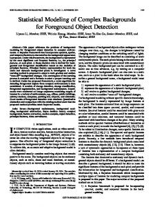
The existence of both the NDF and the one-point PDF of the NDF (!) can be a source for confusion (especially when stochastic solution methods are used to find approximate solutions for the NDF). The reader should keep in mind that the NDF is not a probabilistic quantity, but instead arises due to the infinite possible number of particle sizes present in the system. In contrast, the one-point PDF arises from the statistical modeling approach used to describe turbulent mixing. As mentioned above, QMOM and DQMOM should yield identical results for the statistics of the NDF moments mk . However, from a numerical perspective it is advantageous to use DQMOM. For example, when discretizing the CFD model for the NDF moments in each environment mkn numerical errors (primarily in the convection term) can lead to realizability problems (e.g. m21n > m2nm0n ). Such errors are avoided with DQMOM if the numerical scheme is chosen such that the weights and abscissas are everywhere non-negative. As an example, we consider the application of a two-environment (Ne = 2), four-node (M = 4) CFD model in a 1-D periodic domain 25 that satisfies the following assumptions: (i) the turbulence field is homogeneous and stationary; (ii) the mean velocity is zero everywhere; (iii) the dimensionless length of the domain is two and the 15

Ying Liu, Qing Tang, and Rodney O. Fox 1

0.8

p1

0.6

0.4

0.2

0

0

0.5

1 X

1.5

2

Figure 9: Initial distribution of the inlet streams in the x-direction.

dimensionless turbulent diffusivity is 0.1286. Initially the domain is non-premixed and separated at x = 1 into two parts (Fig. 9). One part contains only environment 1 in which w11 = 0.997, w21 = w31 = w41 = 0.001, v11 = 1, v21 = 2, v31 = 3, and v41 = 4. The other part contains only environment 2 in which w12 = 0.9985, w22 = w32 = w42 = 0.0005, v12 = 0.5, v22 = 1.5, v32 = 2.5, and v42 = 3.5. The initial distribution of p1 across the domain is shown in Fig. 9. As time evolves, the weights and abscissas of each environment change due to mixing and aggregation (Brownian aggregation in this example). Using either QMOM or DQMOM, eight NDF moments are needed for each environment. In Fig. 10 four NDF moments are compared for the two methods. In this example, the first two terms on the right-hand side of Eq. 15 were neglected when we calculated b∗n and c∗n for numerical stability purposes. Any differences between the QMOM and DQMOM results are due to neglecting these terms. Algorithms for treating those two terms stably and accurately are under development. As Fig. 10 shows, NDF moments predicted by DQMOM and QMOM are in close agreement. The distributions of the zero-order NDF moment in the two environments (m0n ) are identical since the initial values of them are identical and aggregation rates are comparable in both environments. The zero-order NDF moments decrease gradually as a result of the decreasing number density due to aggregation. The first-order NDF moment in environment 1 decreases with time, while in environment 2 it increases. Although it is not shown in the figure, the Reynolds-averaged first-order NDF moment (hm1i = p1 m11 + p2 m12) remains constant, indicating that neither mixing nor aggregation changes the total volume of the particles in this closed system. The higher-order NDF moments increase monotonically since the abscissas increase due to aggregation. Nevertheless, the third-order NDF moments increase faster than the second-order NDF moments. Due to micromixing, the NDF moments in the environments approach the Reynolds-average NDF moments at large times. In the example presented above, we considered only aggregation and mixing (i.e. “mesomixing” due to turbulent dispersion and micromixing). In more challenging applications such as soot production 26 there will be a strong coupling between the chemistry (i.e. φ) and the evolution of the NDF. For example, soot will be formed at locations in composi16

Ying Liu, Qing Tang, and Rodney O. Fox

Figure 10: Time evolution of the spatial distribution of the moments mkn (k = 0, . . ., 3) predicted by DQMOM (lines) and QMOM (symbols). Left: Environment 1. Right: Environment 2. Square: initial conditions. Down triangle: t = 0.002. Circle: t = 0.02. Diamond: t = 0.04. Up triangle: t = 0.08.

17

Ying Liu, Qing Tang, and Rodney O. Fox

tion space that are fuel rich and will be oxidized in locations with excess oxygen. It can be anticipated that the successful description of fine-particle formation is such strongly coupled problems will require a detailed CFD model that explicitly accounts for subgrid-scale fluctuations and the correlations between φ and the NDF. 6

CONCLUSIONS

As illustrated in this work, CFD models for single-phase turbulent mixing in chemical reactors are quite advanced and are now available in many commercial CFD codes. As highlighted in the examples, the basic components for successful predictions are accurate models for 1. the turbulent flow field, 2. turbulent scalar transport (dispersion and advection), 3. subgrid-scale fluctuations in the scalar fields (micromixing), 4. chemical/physical processes such as reactions and particle dynamics. If at all possible, each of these model components should be validated independently. In any case, the quality of the overall CFD predictions depend on the accuracy of all component so each of them should be considered carefully. The extension of the CFD models discussed here to multiphase chemical reactors will require the addition of more physics. For example, if instead of fine particles the dispersed phase consists of “large” particles then it no longer suffices to assume that the particle velocity is the same as the fluid velocity. A CFD model for multiphase flows that considers a separate momentum equations for each phase can be used for this purpose. In addition, it will also be important to include accurate models for heat and mass transfer between phases, and chemical reactions inside the phases or at the phase boundaries. As noted in the Introduction, each new reactor type will require an appropriate CFD model that captures the ratecontrolling steps in the overall process. Thus, the field of CFD modeling of chemical reactors still has many new horizons to explore. ACKNOWLEDGMENTS We gratefully acknowledge financial support from the U.S. National Science Foundation through a regular grant (CTS-0336435) and the SBIR Phase I program (DMI-0441833). We would also like to acknowledge our many collaborators with whom we have worked to carry out the research used in the example applications discussed in this work. References [1] R.V. Mehta, J.M. Tarbell. An experimental study of the effect of turbulent mixing on the selectivity of competing reactions, AIChE Journal, 33, 1089–1101, (1987). 18

Ying Liu, Qing Tang, and Rodney O. Fox

[2] J.A. Baldyga, R. Pohorecki. Turbulent micromixing in chemical reactors – a review, Chemical Engineering Journal, 58, 183–195, (1995), [3] J.A. Baldyga, J.R. Bourne. Turbulent mixing and chemical reactions. New York: John Wiley & Sons, (1999). [4] R.O. Fox. Computational Models for Turbulent Reacting Flows, Cambridge University Press, (2003). [5] H. Feng, M.G. Olsen, Y. Liu, R.O. Fox, J.C. Hill. Investigation of turbulent mixing in a confined planar-jet reactor, AIChE Journal, 51, 2649–2664, (2005). [6] H.C. Chen, V.C. Patel. Near-wall turbulence models for complex flows including separation, AIAA Journal, 26, 641–648, (1988). [7] U. Piomelli, J. Ferziger, P. Moin, J. Kim (1989). New approximate boundary conditions for large eddy simulations of wall-bounded flows. Physics of Fluids A , 1, (6), 1061-1068. [8] V. Raman, R.O. Fox, A.D. Harvey, D.H. West. Effect of feed–stream configuration on gas-phase chlorination reactor performance. Industrial & Engineering Chemistry Research, 42, 2544–2557, (2003). [9] V. Raman, R.O. Fox, A.D. Harvey. Hybrid finite-volume/transported PDF simulations of a partially premixed methane-air flame. Combustion and Flame, 136, 327– 350, (2004). [10] L. Wang, R.O. Fox. Comparison of micromixing models for CFD simulation of nanoparticle formation. AIChE J. 2004, 50, 2217–2232, (2004). [11] B.K. Johnson, R.K. Prud’homme. Chemical processing and micromixing in confined impinging jets. AIChE Journal, 49, 2264–2282, (2003). [12] Y. Liu, R.O. Fox. Predictions for chemical processing in a confined impinging-jets reactor. AIChE Journal, 52, 731–744, (2006). [13] A.R. Masri. http://www.mech.eng.usyd.edu.au/research/energy/#data. [14] C.J. Sung, C.K. Law, J-Y Chen. Augmented reduced mechanisms for NO emission in methane oxidation, Combustion and Flame, 125, 906–919, (2001). [15] S.B. Pope. Computationally efficient implementation of combustion chemistry using in situ adaptive tabulation, Combustion Theory and Modelling, 1, 41–63, (1997).

19

Ying Liu, Qing Tang, and Rodney O. Fox

[16] Q. Tang, W. Zhao, M. Bockelie, R.O. Fox. Numerical simulations of turbulent bluffbody flames using multi-environment presumed PDF method with realistic chemistry, Fall Meeting of the Western States Section of the Combustion Institute, Stanford University, Paper 05F-36, (2005). [17] K. Liu, S.B. Pope. Calculations of bluff-body stabilized flames using a joint probability density function model with detailed chemistry, Combustion and Flame, 141, 89–117, (2005). [18] V. Raman, H. Pitsch, R.O. Fox. Eulerian transported probability density function sub-filter model for large-eddy simulations of turbulent combustion, Combustion Theory and Modelling, , (in press), (2006). [19] D. Piton, R.O. Fox, B. Marcant. Simulation of fine particle formation by precipitation using computational fluid dynamics, Canadian Journal of Chemical Engineering, 78, 983–993, (2000). [20] T. Johannessen, S.E. Pratsinis, H. Livbjerg. Computational fluid particle dynamics for the flame synthesis of alumina particles, Chemical Engineering Science, 55, 177– 191, (2000). [21] T. Johannessen, S.E. Pratsinis, H. Livbjerg. Computational analysis of coagulation and coalescence in the flame synthesis of titania particles, Power Technology, 118, 242–250, (2001). [22] R. McGraw. Description of aerosol dynamics by the quadrature method of moments. Aerosol Science and Technology, 27, 255–265 (1997). [23] D.L. Marchisio, R.O Fox. Solution of population balance equations using the direct quadrature method of moments, Journal of Aerosol Science, 36, 43–73, (2005). [24] R.O. Fox. CFD models for analysis and design of chemical reactors. Advances in Chemical Engineering, in press, (2006) [25] L. Wang, R.O. Fox. Application of in situ adaptive tabulation to CFD simulation of nano-particle formation by reactive precipitation, Chemical Engineering Science, 58, 4387–4401, (2003). [26] A. Zucca, D.L. Marchisio, A.A. Barresi, R.O. Fox. Implementation of the population balance equation in CFD codes for modelling soot formation in turbulent flames, Chemical Engineering Science, 61, 87–95, (2006).

20