CFD Module Model Library Manual

CFD Module Model Library Manual

CFD Module Model Library Manual © 1998–2014 COMSOL Protected by U.S. Patents listed on www.comsol.com/patents, and U.S. Patents 7,519,518; 7,596,474; 7,623,991; and 8,457,932. Patents pending. This Documentation and the Programs described herein are furnished under the COMSOL Software License Agreement (www.comsol.com/comsol-license-agreement) and may be used or copied only under the terms of the license agreement. COMSOL, COMSOL Multiphysics, Capture the Concept, COMSOL Desktop, and LiveLink are either registered trademarks or trademarks of COMSOL AB. All other trademarks are the property of their respective owners, and COMSOL AB and its subsidiaries and products are not affiliated with, endorsed by, sponsored by, or supported by those trademark owners. For a list of such trademark owners, see www.comsol.com/trademarks. Version:

October 2014

COMSOL 5.0

Contact Information Visit the Contact COMSOL page at www.comsol.com/contact to submit general inquiries, contact Technical Support, or search for an address and phone number. You can also visit the Worldwide Sales Offices page at www.comsol.com/contact/offices for address and contact information. If you need to contact Support, an online request form is located at the COMSOL Access page at www.comsol.com/support/case. Other useful links include: • Support Center: www.comsol.com/support • Product Download: www.comsol.com/product-download • Product Updates: www.comsol.com/support/updates • Discussion Forum: www.comsol.com/community • Events: www.comsol.com/events • COMSOL Video Gallery: www.comsol.com/video • Support Knowledge Base: www.comsol.com/support/knowledgebase Part number: CM021304

Solved with COMSOL Multiphysics 5.0

Ai r f lo w O v e r an A h m ed Bod y Introduction This model describes how to calculate the turbulent flow field around a simple car-like geometry using the CFD Module’s Turbulent Flow, k-ε physics interface. Detailed instructions guide you through the different steps of the modeling process in COMSOL Multiphysics.

Model Definition The Ahmed body represents a simplified, ground vehicle geometry of a bluff body type. Its shape is simple enough to allow for accurate flow simulation but retains some important practical features relevant to automobile bodies. The geometry was first defined by Ahmed, who also measured its aerodynamic properties in wind-tunnel experiments (Ref. 1). Further experiments have also been performed by Lienhart and Becker (Ref. 2). The Ahmed body has become a popular benchmark case for RANS models (Ref. 3). GEOMETRY

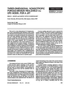
The Ahmed body is presented in Figure 1. The total length (L) of the body is 1.044 m from front to end. It is 0.288 m in height and 0.389 m in width. Cylindrical legs 0.05 m in length are attached to the bottom surface. The angle of the rear slanting surface is typically varied between 0 and 40 degrees. This particular geometry has a

1 |

AIRFLOW OVER AN AHMED BODY


slant angle of 25 degrees, which is the same slant angle used in Ref. 3.

Length

Width

Height

Figure 1: Ahmed body with 25 degree slant of the rear face. The body is placed in a flow domain that is 8L-by-2L-by-2L (length-by-width-by-height), with its front positioned 2L from the flow inlet face. Mirror symmetry reduces the computational domain by half, as shown in Figure 2.

Outlet

Slip 8L

Symmetry

Wall function

L

Inlet

2L

2L

Figure 2: The size of the computational domain is reduced by mirror symmetry.

2 |



TU R B U L E N C E M O D E L

The Reynolds number based on the length of the body, L, and the inlet velocity is 2.77·106 which means that the flow is turbulent. The k-ε turbulence model will be applied to account for the turbulence. The k-ε turbulence model is described in Theory for the Turbulent Flow Interfaces in the CFD Module User’s Guide. BOUNDARY CONDITIONS

Air enters the computational domain at a freestream velocity u∞=40 m/s normal to the inlet surface. Experimental inlet conditions from Ref. 3 are used for the velocity and turbulent kinetic energy. To obtain a condition for ε, Ref. 3 suggests to set μT=10·μ at the inlet. At the outlet, a Pressure condition is applied. The floor of the flow domain and surface of the Ahmed body are described by wall functions. Wall functions could also be applied to the outer wall and the ceiling of the wind tunnel. Their main effect on the flow around the body is however to keep the flow contained, and it will therefore suffice to model them as slip walls. The temperature is assumed to be 293 K and the reference pressure is 1 atm. MESHING

A common mesh size in Ref. 3 is half a million cells for simulations with wall functions. However, those simulations do not include the stilts (the legs that support the body), and the computational domains are smaller. Hence, you can expect to need an even larger mesh in this simulation to resolve the flow. How large is however difficult to know in advance. There are two important aspects of the meshing. The first is to resolve the flow in the wake. To achieve this, additional mesh control entities are introduced in the geometry. These entities are advantageous to normal geometrical entities since they are removed whence they are completely meshed. A smoothing algorithm will then smooth the mesh locally in order to minimize gradients in the mesh size. Also, it is easier to introduce boundary layer mesh when the control entities are removed.

Results and Discussion A key figure for the Ahmed body is the total drag coefficient, CD, which is defined as ρu ∞ F-----= C D ----------2 Ap 2

(1)

3 |



where F is the total drag force on the body, Ap is area of the body projected on a plane perpendicular to the flow direction (that is, the xz-plane), ρ is the density (approximately equal to 1.2 kg/m3), and u∞ is the freestream velocity (equal to 40 m/ s). Ap can be calculated from geometrical data and is equal to 0.115 m2 including the stilts. The contributions to CD are commonly reported as the pressure coefficients on front, slant, and base and the skin friction drag coefficient. These numbers are given in Table 1. Note that the numbers given by the postprocessing tools correspond to half the body, and hence, Ap must be replaced by Ap/2 when calculating the entries of Table 1. TABLE 1: DRAG COEFFICIENTS CP FRONT

CP SLANT

CP BASE

SKIN FRICTION

TOTAL DRAG

Measurements

0.020

0.140

0.070

0.055

0.285

k-ε

0.039

0.109

0.073

0.039

0.282

As can be seen, most contributions are in reasonable agreements with experiments. The total drag is very well predicted, but the individual contributions deviate from experimental values. The pressure coefficient on the front is too high and the skin friction too low. Ref. 4 uses two different versions of the k-e model and two different wall function formulations and all combinations show this behavior. It can probably be attributed to the fact that wall functions are not very good at predicting the transition observed in the experiments to take place on the front and roof of the body. The low value of the slant pressure drag coefficient can be understood by looking at Figure 3, which shows streamlines in the symmetry plane. Experimental results indicate that the flow along the slant is attached almost everywhere and that there are two small recirculation regions behind the base. The computational results capture this behavior, but the extent of the recirculation zones is somewhat overpredicted. The pressure drag coefficient, especially for the slant, is very sensitive to the exact shape and location of the recirculation regions.

4 |



Figure 3: Streamlines in the symmetry plane. Figure 4 shows a 3D plot of the streamlines behind the Ahmed body. The thickness of the lines is given by the turbulent kinetic energy. The most notable feature of the flow field is an “empty” region behind the body. The streamlines on the edge of the region are thick but with low velocity magnitude. This region is constituted of the recirculation vortices visible in Figure 3. The region ends when vortices from the

5 |



trailing edges of the body merge into two counter rotating vortices (only one vortex is visible because the other vortex is on the other side of the symmetry plane).

Figure 4: Streamlines behind the Ahmed body. The streamlines are colored by the velocity magnitude and their thickness is proportional to the turbulent kinetic energy.

6 |



More details are visible in Figure 5 and Figure 6, which show arrow plots of the velocity in the xz-plane 80 mm and 200 mm downstream of the body, respectively.

Figure 5: Velocity in the xz-plane at y = L + 0.08 m. The flow pattern 80 mm downstream of the body shows two major vortices, one emanating from the outer edge of the slant and one emanating from the interaction between the floor and the stilts. The flow is qualitatively equal to the experimental results (Ref. 2). There are however quantitative differences. The upper vortex is smaller

7 |



compared to experiments while the lower vortex is more pronounced than in the experiments.

Figure 6: Velocity in the xz-plane at y = L + 0.20 m. The flow pattern 200 mm downstream of the body shows that one major vortex is beginning to form but remains of the separate vortices can still be detected. The formation is, however, not proceeded as far as in the experiments. In conclusion, the major features of the flow are well captured by the k-ε model, but there are details that deviate from experimental data. This finding is in agreement with other RANS simulations of the Ahmed body (Ref. 3).

References 1. S.R. Ahmed, G. Ramm, and G. Faltin, “Some Salient Features of the Time-Averaged Ground Vehicle Wake,” SAE Technical Paper 840300, 1984. 2. H. Lienhart and S. Becker, “Flow and Turbulence Structure in the Wake of a Simplified Car Model,” SAE 2003 World Congress, SAE Paper 2003-01-0656, Detroit, Michigan, 2003.

8 |



3. 9th ERCOFTAC/IAHR Workshop on Refined Turbulence Modelling, Darmstadt University of Technology, Germany, 2001. 4. T.J. Craft, S.E. Gant, H. Iacovides, B.E. Launder, and C.M.E. Robinson, “Computational Study of Flow Around the ‘Ahmed’ Car Body”, 9th ERCOFTAC/ IAHR Workshop on Refined Turbulence Modelling, 2001.

Model Library path: CFD_Module/Single-Phase_Benchmarks/ahmed_body

Modeling Instructions From the File menu, choose New. NEW

1 In the New window, click Model Wizard. MODEL WIZARD

1 In the Model Wizard window, click 3D. 2 In the Select physics tree, select Fluid Flow>Single-Phase Flow>Turbulent Flow>Turbulent Flow, k-ε (spf). 3 Click Add. 4 Click Study. 5 In the Select study tree, select Preset Studies>Stationary. 6 Click Done. DEFINITIONS

Parameters 1 On the Model toolbar, click Parameters. 2 In the Settings window for Parameters, locate the Parameters section. 3 In the table, enter the following settings: Name

Expression

Value

Description

L

1.044[m]

1.044 m

Body length

D

0.389[m]

0.3890 m

Body width

H_body

0.288[m]

0.2880 m

Body height

9 |



Name

Expression

Value

Description

Cl

0.05[m]

0.05000 m

Clearance

Sl

0.222[m]

0.2220 m

Slant length

Sb

H_body+Cl-Sl*s in(25[deg])

0.2442 m

Slant base

Rl

L-Sl*cos(25[de g])

0.8428 m

Roof length

Interpolation 1 (int1) 1 On the Model toolbar, click Functions and choose Global>Interpolation. 2 In the Settings window for Interpolation, locate the Definition section. 3 From the Data source list, choose File. 4 Click Browse. 5 Browse to the model’s Model Library folder and double-click the file ahmed_body_Uin.txt.

6 Click Import. 7 Find the Functions subsection. In the table, enter the following settings: Function name

Position in file

Uin

1

8 Locate the Interpolation and Extrapolation section. From the Extrapolation list,

choose Specific value. 9 Locate the Units section. In the Arguments text field, type m. 10 In the Function text field, type m/s.

Interpolation 2 (int2) 1 On the Model toolbar, click Functions and choose Global>Interpolation. 2 In the Settings window for Interpolation, locate the Definition section. 3 From the Data source list, choose File. 4 Click Browse. 5 Browse to the model’s Model Library folder and double-click the file ahmed_body_Vin.txt.

6 Click Import.

10 |



7 Find the Functions subsection. In the table, enter the following settings: Function name

Position in file

Vin

1

8 Locate the Units section. In the Arguments text field, type m. 9 In the Function text field, type m/s.

Interpolation 3 (int3) 1 On the Model toolbar, click Functions and choose Global>Interpolation. 2 In the Settings window for Interpolation, locate the Definition section. 3 From the Data source list, choose File. 4 Click Browse. 5 Browse to the model’s Model Library folder and double-click the file ahmed_body_Win.txt.

6 Click Import. 7 Find the Functions subsection. In the table, enter the following settings: Function name

Position in file

Win

1

8 Locate the Interpolation and Extrapolation section. From the Extrapolation list,

choose Specific value. 9 Locate the Units section. In the Arguments text field, type m. 10 In the Function text field, type m/s.

Interpolation 4 (int4) 1 On the Model toolbar, click Functions and choose Global>Interpolation. 2 In the Settings window for Interpolation, locate the Definition section. 3 From the Data source list, choose File. 4 Click Browse. 5 Browse to the model’s Model Library folder and double-click the file ahmed_body_kin.txt.

6 Click Import.

11 |



7 Find the Functions subsection. In the table, enter the following settings: Function name

Position in file

kin

1

8 Locate the Units section. In the Arguments text field, type m. 9 In the Function text field, type m^2/s^2. GEOMETRY 1

Import 1 (imp1) 1 On the Model toolbar, click Import. 2 In the Settings window for Import, locate the Import section. 3 Click Browse. 4 Browse to the model’s Model Library folder and double-click the file ahmed_body.mphbin.

5 Click Import. 6 Click the Zoom Extents button on the Graphics toolbar.

Block 1 (blk1) 1 On the Geometry toolbar, click Block. 2 In the Settings window for Block, locate the Size section. 3 In the Width text field, type 2*L. 4 In the Depth text field, type 8*L. 5 In the Height text field, type 2*L. 6 Locate the Position section. In the x text field, type -L. 7 In the y text field, type -2*L. 8 Right-click Component 1 (comp1)>Geometry 1>Block 1 (blk1) and choose Build Selected. 9 Click the Go to Default 3D View button on the Graphics toolbar.

Block 2 (blk2) 1 On the Geometry toolbar, click Block. 2 In the Settings window for Block, locate the Size section. 3 In the Width text field, type L. 4 In the Depth text field, type 8*L.

12 |



5 In the Height text field, type 2*L. 6 Locate the Position section. In the x text field, type -L. 7 In the y text field, type -2*L. 8 Right-click Component 1 (comp1)>Geometry 1>Block 2 (blk2) and choose Build Selected.

Difference 1 (dif1) 1 On the Geometry toolbar, click Booleans and Partitions and choose Difference. 2 Select the object blk1 only. 3 In the Settings window for Difference, locate the Difference section. 4 Find the Objects to subtract subsection. Select the Active toggle button. 5 Select the objects blk2 and imp1 only. 6 Right-click Component 1 (comp1)>Geometry 1>Difference 1 (dif1) and choose Build Selected.

Cylinder 1 (cyl1) 1 On the Geometry toolbar, click Cylinder. 2 In the Settings window for Cylinder, locate the Size and Shape section. 3 In the Radius text field, type 2.2*L. 4 In the Height text field, type L. 5 Locate the Position section. In the y text field, type 0.2*L. 6 In the z text field, type -0.1*L. 7 Locate the Axis section. From the Axis type list, choose x-axis.

Convert to Surface 1 (csur1) 1 On the Geometry toolbar, click Conversions and choose Convert to Surface. 2 Select the object cyl1 only. 3 Click the Wireframe Rendering button on the Graphics toolbar.

Delete Entities 1 (del1) 1 In the Model Builder window, right-click Geometry 1 and choose Delete Entities. 2 On the object csur1, select Boundaries 1 and 3–6 only.

These are all surfaces of the cylinder, except the curved surface behind the body. 3 Right-click Component 1 (comp1)>Geometry 1>Delete Entities 1 (del1) and choose Build Selected.

13 |



Union 1 (uni1) 1 On the Geometry toolbar, click Booleans and Partitions and choose Union. 2 Select the objects dif1 and del1 only. 3 Right-click Component 1 (comp1)>Geometry 1>Union 1 (uni1) and choose Build Selected.

Delete Entities 2 (del2) 1 Right-click Geometry 1 and choose Delete Entities. 2 On the object uni1, select Boundaries 10 and 16 only.

These are the boundaries that protrude above and beneath the channel. 3 Right-click Component 1 (comp1)>Geometry 1>Delete Entities 2 (del2) and choose Build Selected.

Hexahedron 1 1 On the Geometry toolbar, click More Primitives and choose Hexahedron. 2 In the Settings window for Hexahedron, locate the Vertices section. 3 In row 1, set y to L, and set z to Cl. 4 In row 2, set y to 2*L, and set z to Cl. 5 In row 3, set x to D/2, set y to 2*L, and set z to Cl. 6 In row 4, set x to D/2, set y to L, and set z to Cl. 7 In row 5, set y to L, and set z to Sb. 8 In row 6, set y to 2*L, and set z to Sb. 9 In row 7, set x to D/2, set y to 2*L, and set z to Sb. 10 In row 8, set x to D/2, set y to L, and set z to Sb.

Hexahedron 2 1 On the Geometry toolbar, click More Primitives and choose Hexahedron. 2 In the Settings window for Hexahedron, locate the Vertices section. 3 In row 1, set y to L, and set z to Sb. 4 In row 2, set y to 2*L, and set z to Sb. 5 In row 3, set x to D/2, set y to 2*L, and set z to Sb. 6 In row 4, set x to D/2, set y to L, and set z to Sb. 7 In row 5, set y to L, and set z to H_body+Cl+0.01[m]. 8 In row 6, set y to 2*L, and set z to H_body+Cl+0.01[m]. 9 In row 7, set x to D/2, set y to 2*L, and set z to H_body+Cl+0.01[m].

14 |



10 In row 8, set x to D/2, set y to L, and set z to H_body+Cl+0.01[m].

Hexahedron 3 1 On the Geometry toolbar, click More Primitives and choose Hexahedron. 2 In the Settings window for Hexahedron, locate the Vertices section. 3 In row 1, set y to L, and set z to Sb. 4 In row 2, set y to L, and set z to H_body+Cl+0.01[m]. 5 In row 3, set x to D/2, set y to L, and set z to H_body+Cl+0.01[m]. 6 In row 4, set x to D/2, set y to L, and set z to Sb. 7 In row 5, set y to Rl, and set z to H_body+Cl. 8 In row 6, set y to Rl, and set z to H_body+Cl+0.01[m]. 9 In row 7, set x to D/2, set y to Rl, and set z to H_body+Cl+0.01[m]. 10 In row 8, set x to D/2, set y to Rl, and set z to H_body+Cl.

Union 2 (uni2) 1 On the Geometry toolbar, click Booleans and Partitions and choose Union. 2 Select the objects hex1, hex2, and hex3 only. 3 In the Settings window for Union, locate the Union section. 4 Clear the Keep interior boundaries check box.

Ignore Edges 1 (ige1) 1 On the Geometry toolbar, click Virtual Operations and choose Ignore Edges. 2 On the object fin, select Edges 26, 27, 30, 34, 44, 49, 54, 55, 64, and 65 only.

Mesh Control Domains 1 (mcd1) 1 On the Geometry toolbar, click Virtual Operations and choose Mesh Control Domains. 2 On the object ige1, select Domain 2 only.

Mesh Control Faces 1 (mcf1) 1 On the Geometry toolbar, click Virtual Operations and choose Mesh Control Faces. 2 On the object mcd1, select Boundary 12 only. 3 On the Geometry toolbar, click Build All. 4 Click the Zoom Extents button on the Graphics toolbar. 5 Click the Go to Default 3D View button on the Graphics toolbar. 6 In the Model Builder window, collapse the Geometry 1 node.

15 |



7 Click the Transparency button on the Graphics toolbar to return to the default state.

The model geometry is now complete.

Create an explicit selection of the boundaries of the body. DEFINITIONS

Explicit 1 1 On the Definitions toolbar, click Explicit. 2 In the Settings window for Explicit, locate the Input Entities section. 3 From the Geometric entity level list, choose Boundary. 4 Click the Select Box button on the Graphics toolbar. 5 Select Boundaries 5–11 and 13–16 only. 6 Right-click Component 1 (comp1)>Definitions>Explicit 1 and choose Rename. 7 In the Rename Explicit dialog box, type Body in the New label text field. 8 Click OK. 9 Click the Transparency button on the Graphics toolbar. ADD MATERIAL

1 On the Model toolbar, click Add Material to open the Add Material window. 2 Go to the Add Material window.

16 |



3 In the tree, select Built-In>Air. 4 Click Add to Component in the window toolbar. 5 On the Model toolbar, click Add Material to close the Add Material window. Turbulent Flow, k-ε (spf)

Wall 2 1 On the Physics toolbar, click Boundaries and choose Wall. 2 In the Settings window for Wall, locate the Boundary Condition section. 3 From the Boundary condition list, choose Slip. 4 Select Boundaries 4 and 17 only.

Symmetry 1 1 On the Physics toolbar, click Boundaries and choose Symmetry. 2 Select Boundary 1 only.

Inlet 1 1 On the Physics toolbar, click Boundaries and choose Inlet. 2 Select Boundary 2 only. 3 In the Settings window for Inlet, locate the Turbulence Conditions section. 4 Click the Specify turbulence variables button. 5 In the k0 text field, type kin(x,z). 6 In the ε0 text field, type spf.C_mu*kin(x,z)^2*spf.rho/ (10*1.814e-5[Pa*s]).

7 Locate the Velocity section. Click the Velocity field button. 8 Specify the u0 vector as Uin(x,z)

x

Vin(x,z)

y

Win(x,z)

z

Change to unidirectional constraints to avoid reaction forces in the pressure from the constraint for ε. 9 In the Model Builder window’s toolbar, click the Show button and select Advanced Physics Options in the menu. 10 Click to expand the Constraint settings section. Locate the Constraint Settings

section. From the Apply reaction terms on list, choose Individual dependent variables.

17 |



Outlet 1 1 On the Physics toolbar, click Boundaries and choose Outlet. 2 Select Boundary 12 only. MESH 1

Size 1 In the Model Builder window, under Component 1 (comp1) right-click Mesh 1 and

choose Edit Physics-Induced Sequence. 2 In the Model Builder window, under Component 1 (comp1)>Mesh 1 click Size. 3 In the Settings window for Size, locate the Element Size section. 4 Click the Custom button. 5 Locate the Element Size Parameters section. In the Maximum element size text field,

type 0.1. 6 In the Minimum element size text field, type 0.0025. 7 In the Curvature factor text field, type 0.4. 8 In the Resolution of narrow regions text field, type 0.5.

Size 1 1 In the Model Builder window, under Component 1 (comp1)>Mesh 1 click Size 1. 2 In the Settings window for Size, locate the Geometric Entity Selection section. 3 Click Clear Selection. 4 Select Boundaries 23, 25, and 27 only. 5 Locate the Element Size section. Click the Custom button. 6 Locate the Element Size Parameters section. Select the Maximum element size check

box. 7 In the associated text field, type 0.05. 8 Click the Build Selected button.

Size 2 1 In the Model Builder window, right-click Mesh 1 and choose Size. 2 In the Settings window for Size, locate the Geometric Entity Selection section. 3 From the Geometric entity level list, choose Boundary. 4 Select Boundary 3 only. 5 Locate the Element Size section. Click the Custom button.

18 |



6 Locate the Element Size Parameters section. Select the Maximum element size check

box. 7 In the associated text field, type 0.035.

Size 3 1 Right-click Mesh 1 and choose Size. 2 In the Settings window for Size, locate the Geometric Entity Selection section. 3 From the Geometric entity level list, choose Boundary. 4 Select Boundaries 10 and 11 only. 5 Locate the Element Size section. Click the Custom button. 6 Locate the Element Size Parameters section. Select the Maximum element size check


Size 4 1 Right-click Mesh 1 and choose Size. 2 In the Settings window for Size, locate the Geometric Entity Selection section. 3 From the Geometric entity level list, choose Boundary. 4 Select Boundaries 5–9, 13, and 16 only. 5 Locate the Element Size section. Click the Custom button. 6 Locate the Element Size Parameters section. Select the Maximum element size check


Size 5 1 Right-click Mesh 1 and choose Size. 2 In the Settings window for Size, locate the Geometric Entity Selection section. 3 From the Geometric entity level list, choose Edge. 4 Select Edges 35 and 36 only. 5 Locate the Element Size section. Click the Custom button. 6 Locate the Element Size Parameters section. Select the Maximum element size check


19 |



Free Tetrahedral 1 1 In the Model Builder window, under Component 1 (comp1)>Mesh 1 right-click Corner Refinement 1 and choose Disable. 2 In the Model Builder window, under Component 1 (comp1)>Mesh 1 click Free Tetrahedral 1. 3 In the Settings window for Free Tetrahedral, locate the Domain Selection section. 4 Click Clear Selection. 5 Select Domain 3 only.

Size 1 1 Right-click Component 1 (comp1)>Mesh 1>Free Tetrahedral 1 and choose Size. 2 In the Settings window for Size, locate the Element Size section. 3 Click the Custom button. 4 Locate the Element Size Parameters section. Select the Maximum element growth rate

check box. 5 In the associated text field, type 1.03.

Free Tetrahedral 1 Right-click Free Tetrahedral 1 and choose Build Selected.

Free Tetrahedral 2 1 Right-click Mesh 1 and choose Free Tetrahedral. 2 In the Settings window for Free Tetrahedral, locate the Domain Selection section. 3 From the Geometric entity level list, choose Domain. 4 Select Domain 1 only. 5 Click the Build Selected button.

Boundary Layers 1 1 In the Model Builder window, under Component 1 (comp1)>Mesh 1 click Boundary Layers 1. 2 In the Settings window for Boundary Layers, locate the Domain Selection section. 3 Click Clear Selection. 4 Select Domain 1 only.

Boundary Layer Properties 1 1 In the Model Builder window, expand the Boundary Layers 1 node, then click Boundary Layer Properties 1.

20 |



2 In the Settings window for Boundary Layer Properties, locate the Boundary Layer Properties section. 3 In the Number of boundary layers text field, type 6. 4 In the Thickness adjustment factor text field, type 1.5.

Boundary Layers 1 In the Model Builder window, under Component 1 (comp1)>Mesh 1 right-click Boundary Layers 1 and choose Build Selected.

Swept 1 1 Right-click Mesh 1 and choose Swept. 2 In the Settings window for Swept, locate the Domain Selection section. 3 From the Geometric entity level list, choose Domain. 4 Select Domain 2 only.

Distribution 1 1 Right-click Component 1 (comp1)>Mesh 1>Swept 1 and choose Distribution. 2 In the Settings window for Distribution, locate the Distribution section. 3 From the Distribution properties list, choose Predefined distribution type. 4 In the Number of elements text field, type 28. 5 In the Element ratio text field, type 6. 6 In the Model Builder window, right-click Mesh 1 and choose Free Tetrahedral. 7 Right-click Mesh 1 and choose Build All. 8 In the Model Builder window, collapse the Mesh 1 node. COMPONENT 1 (COMP1)

On the Mesh toolbar, click Add Mesh. MESH 2

Reference 1 1 In the Model Builder window, under Component 1 (comp1)>Meshes right-click Mesh 2

and choose More Operations>Reference. 2 In the Settings window for Reference, locate the Reference section. 3 From the Mesh list, choose Mesh 1.

Scale 1 1 Right-click Component 1 (comp1)>Meshes>Mesh 2>Reference 1 and choose Scale.

21 |



2 In the Settings window for Scale, locate the Scale section. 3 In the Element size scale text field, type 2. 4 In the Model Builder window, right-click Mesh 2 and choose Build All. 5 In the Model Builder window, collapse the Mesh 2 node. COMPONENT 1 (COMP1)

On the Mesh toolbar, click Add Mesh. MESH 3

Reference 1 1 In the Model Builder window, under Component 1 (comp1)>Meshes right-click Mesh 3

and choose More Operations>Reference. 2 In the Settings window for Reference, locate the Reference section. 3 From the Mesh list, choose Mesh 2.

Scale 1 1 Right-click Component 1 (comp1)>Meshes>Mesh 3>Reference 1 and choose Scale. 2 In the Settings window for Scale, locate the Scale section. 3 In the Element size scale text field, type 2. 4 In the Model Builder window, right-click Mesh 3 and choose Build All. 5 In the Model Builder window, collapse the Mesh 3 node. COMPONENT 1 (COMP1)

1 In the Model Builder window, collapse the Component 1 (comp1)>Meshes node.

Show advanced study options to be able to apply the manual multigrid levels. 2 In the Model Builder window’s toolbar, click the Show button and select Advanced Study Options in the menu. STUDY 1

Step 1: Stationary 1 In the Model Builder window, expand the Study 1 node. 2 Right-click Step 1: Stationary and choose Multigrid Level. 3 In the Settings window for Multigrid Level, locate the Mesh Selection section.

22 |



4 In the table, enter the following settings: Geometry

Mesh

Geometry 1

mesh2

5 In the Model Builder window, right-click Step 1: Stationary and choose Multigrid Level.

Solution 1 1 On the Study toolbar, click Show Default Solver. 2 In the Model Builder window, expand the Solution 1 node. 3 In the Model Builder window, expand the Study 1>Solver Configurations>Solution 1>Stationary Solver 1>Iterative 1 node, then click Multigrid 1. 4 In the Settings window for Multigrid, locate the General section. 5 From the Hierarchy generation method list, choose Manual. 6 In the Model Builder window, collapse the Study 1>Solver Configurations>Solution 1>Stationary Solver 1>Iterative 1 node. 7 In the Model Builder window, expand the Study 1>Solver Configurations>Solution 1>Stationary Solver 1>Iterative 2 node, then click Multigrid 1. 8 In the Settings window for Multigrid, locate the General section. 9 From the Hierarchy generation method list, choose Manual. 10 In the Model Builder window, collapse the Study 1>Solver Configurations>Solution 1>Stationary Solver 1>Iterative 2 node. 11 In the Model Builder window, collapse the Study 1>Solver Configurations>Solution 1>Stationary Solver 1 node. 12 In the Model Builder window, collapse the Solution 1 node. 13 On the Study toolbar, click Compute. RESULTS

Velocity (spf) It is advisable to disable the automatic plot update when working with large 3D models. 1 In the Model Builder window, click Results. 2 In the Settings window for Results, locate the Result Settings section. 3 Clear the Automatic update of plots check box.

23 |



Investigate the lift-off in viscous units to verify that the wall resolution is sufficient. RESULTS

Wall Resolution (spf) 1 On the 3D plot group toolbar, click Plot.

The wall lift-off is larger than 11.06 at some locations, but it is close to 11.06 on most of the body and can hence be considered to be acceptable.

Figure 7: Wall lift-off in viscous units.

Velocity (spf) 1 In the Model Builder window, expand the Results>Velocity (spf) node, then click Slice 1. 2 In the Settings window for Slice, locate the Plane Data section. 3 From the Entry method list, choose Coordinates. 4 In the x-coordinates text field, type 0.15. 5 On the 3D plot group toolbar, click Plot.

The slice plot of the velocity clearly shows the recirculation zone behind the body. The result looks smooth which further supports the assumption that the resolution is acceptable.

24 |



Figure 8: Slice plot at x=0.15 m of the velocity magnitude. To evaluate the input to calculate the entries in Table 1, perform the following steps: RESULTS

Derived Values 1 On the Results toolbar, click More Derived Values and choose Integration>Surface Integration. 2 In the Settings window for Surface Integration, locate the Expression section. 3 In the Expression text field, type nymesh*p. 4 Select Boundaries 5–7 and 13 only. 5 Click the Evaluate button. 6 Locate the Selection section. Click Clear Selection. 7 Select Boundary 10 only. 8 Click the Evaluate button. 9 Click Clear Selection. 10 Select Boundary 11 only.

25 |



11 Click the Evaluate button. 12 From the Selection list, choose Body. 13 Click the Evaluate button. 14 On the Results toolbar, click More Derived Values and choose Integration>Surface Integration. 15 Click the Wireframe Rendering button on the Graphics toolbar. 16 In the Settings window for Surface Integration, locate the Selection section. 17 From the Selection list, choose Body. 18 Locate the Expression section. In the Expression text field, type spf.rho*spf.u_tau*((v-spf.nymesh*(u*spf.nxmesh+v*spf.nymesh+w*spf .nzmesh)))/spf.uPlus.

The wall function expression will be used directly for maximum accuracy. 19 Click the Evaluate button. RESULTS

The following steps reproduce Figure 3:

Data Sets 1 On the Results toolbar, click More Data Sets and choose Surface. 2 In the Settings window for Surface, locate the Parameterization section. 3 From the x- and y-axes list, choose yz-plane. 4 Select Boundary 1 only.

2D Plot Group 4 1 On the Results toolbar, click 2D Plot Group. 2 In the Settings window for 2D Plot Group, locate the Data section. 3 From the Data set list, choose Surface 3. 4 Right-click Results>2D Plot Group 4 and choose Streamline. 5 In the Settings window for Streamline, locate the Expression section. 6 In the x component text field, type v. 7 In the y component text field, type w. 8 Locate the Streamline Positioning section. In the Points text field, type 31. 9 On the 2D plot group toolbar, click Plot.

The following steps reproduce Figure 4:

26 |



Data Sets 1 On the Results toolbar, click More Data Sets and choose Solution. 2 On the Results toolbar, click Selection. 3 In the Settings window for Selection, locate the Geometric Entity Selection section. 4 From the Geometric entity level list, choose Boundary. 5 From the Selection list, choose Body. 6 Select Boundaries 3, 5–11, and 13–16 only.

3D Plot Group 5 1 On the Results toolbar, click 3D Plot Group. 2 In the Model Builder window, under Results right-click 3D Plot Group 5 and choose Surface. 3 In the Settings window for Surface, locate the Data section. 4 From the Data set list, choose Study 1/Solution 1 (2). 5 Locate the Expression section. In the Expression text field, type 1. 6 Locate the Coloring and Style section. Clear the Color legend check box. 7 From the Coloring list, choose Uniform. 8 From the Color list, choose Gray. 9 Clear the Plot data set edges check box. 10 Right-click Results>3D Plot Group 5 and choose Streamline. 11 In the Settings window for Streamline, locate the Streamline Positioning section. 12 From the Positioning list, choose Start point controlled. 13 From the Entry method list, choose Coordinates. 14 In the x text field, type range(0.01,0.03,0.16) range(0.01,0.03,0.16) range(0.01,0.03,0.16) range(0.01,0.03,0.16) range(0.01,0.03,0.16).

15 In the y text field, type -0.5*L. 16 In the z text field, type 0.02*1^range(1,6) 0.08*1^range(1,6) 0.14*1^range(1,6)

0.2*1^range(1,6)

0.26*1^range(1,6).

17 Locate the Coloring and Style section. From the Line type list, choose Tube. 18 In the Tube radius expression text field, type k*1[s^2/m]. 19 Select the Radius scale factor check box. 20 In the associated text field, type 3e-4. 21 Right-click Results>3D Plot Group 5>Streamline 1 and choose Color Expression.

27 |



22 On the 3D plot group toolbar, click Plot.

The following steps will reproduce figures Figure 5 and Figure 6:

Data Sets 1 On the Results toolbar, click Cut Plane. 2 In the Settings window for Cut Plane, locate the Plane Data section. 3 From the Plane list, choose zx-planes. 4 In the y-coordinate text field, type L+0.08. 5 On the Results toolbar, click Cut Plane. 6 In the Settings window for Cut Plane, locate the Plane Data section. 7 From the Plane list, choose zx-planes. 8 In the y-coordinate text field, type L+0.2.

3D Plot Group 6 1 On the Results toolbar, click 3D Plot Group. 2 In the Settings window for 3D Plot Group, locate the Plot Settings section. 3 Clear the Plot data set edges check box.

3D Plot Group 6 1 In the Model Builder window, under Results>3D Plot Group 5 right-click Surface 1 and

choose Copy. 2 Right-click 3D Plot Group 6 and choose Paste Surface. 3 Right-click 3D Plot Group 6 and choose Arrow Surface. 4 In the Settings window for Arrow Surface, locate the Data section. 5 From the Data set list, choose Cut Plane 1. 6 Locate the Expression section. In the y component text field, type 0. 7 Locate the Coloring and Style section. From the Arrow length list, choose Logarithmic. 8 In the Range quotient text field, type 500. 9 Select the Scale factor check box. 10 In the associated text field, type 1.25e-3. 11 In the Number of arrows text field, type 2500. 12 From the Color list, choose Black. 13 Right-click Results>3D Plot Group 6>Arrow Surface 1 and choose Filter. 14 In the Settings window for Filter, locate the Element Selection section.

28 |



15 In the Logical expression for inclusion text field, type (xMultiphase Flow>Bubbly Flow>Turbulent Bubbly Flow (bf). 3 Click Add. 4 Click Study. 5 In the Select study tree, select Preset Studies>Time Dependent. 6 Click Done. DEFINITIONS

First, define some model parameters.

8 |

FLOW IN AN AIRLIFT LOOP REACTOR



Expression

Value

Description

H

1.75[m]

1.750 m

Reactor height

W

0.5[m]

0.5000 m

Reactor width

T

0.08[m]

0.08000 m

Reactor thickness

d_b

3e-3[m]

0.003000 m

Bubble diameter

R

0.02[m]

0.02000 m

Frit radius

L

0.16[m]

0.1600 m

Width of riser and downcomer channels

V_in

0.015[m/s]

0.01500 m/s

Inlet velocity

Cw

5e4[kg/ (m^3*s)]

5.000E4 kg/ (m³·s)

Slip-velocity proportionality constant

rhog_in

0.9727[kg/ (m^3)]

0.9727 kg/m³

Gas density at inlet

GEOMETRY 1

Create the geometry. To simplify this step, insert a prepared geometry sequence. 1 On the Geometry toolbar, click Insert Sequence. 2 Browse to the model’s Model Library folder and double-click the file airlift_loop_reactor.mph.

3 Then click Build all on the Geometry toolbar.

Full geometry instructions can be found and the end of the document. Now pick up the materials from the Material Library. ADD MATERIAL

1 On the Model toolbar, click Add Material to open the Add Material window. 2 Go to the Add Material window. 3 In the tree, select Built-In>Air. 4 Click Add to Component in the window toolbar.

9 |



ADD MATERIAL

1 Go to the Add Material window. 2 In the tree, select Built-In>Water, liquid. 3 Click Add to Component in the window toolbar. 4 On the Model toolbar, click Add Material to close the Add Material window. TU R B U L E N T B U B B L Y F L OW ( B F )

Fluid Properties 1 1 In the Model Builder window, expand the Turbulent Bubbly Flow (bf) node, then click Fluid Properties 1. 2 In the Settings window for Fluid Properties, locate the Materials section. 3 From the Liquid list, choose Water, liquid (mat2). 4 From the Gas list, choose Air (mat1). 5 Locate the Gas Properties section. From the ρg list, choose Calculate from ideal gas law. 6 In the db text field, type d_b. 7 Locate the Slip Model section. From the Slip model list, choose Pressure-drag balance. 8 From the Drag coefficient model list, choose Large bubbles. 9 In the Model Builder window, click Turbulent Bubbly Flow (bf). 10 In the Settings window for Turbulent Bubbly Flow, locate the Physical Model section. 11 Clear the Low gas concentration check box. 12 Click to expand the Turbulence model parameters section. Locate the Turbulence Model Parameters section. In the Cε text field, type 1.4. 13 In the Ck text field, type 0.6.

Gravity 1 1 On the Physics toolbar, click Domains and choose Gravity. 2 Select Domain 1 only.

Wall 2 1 On the Physics toolbar, click Boundaries and choose Wall. 2 Click the Zoom Extents button on the Graphics toolbar. 3 Select Boundaries 6 and 7 only. 4 In the Settings window for Wall, locate the Gas Boundary Condition section.

10 |



5 From the Gas boundary condition list, choose Gas flux. 6 In the Nρgφg text field, type V_in*rhog_in*flc1hs(t[1/s]-5,5).

Here the built-in smoothed Heaviside function flc1hs is used to give a smooth initial value.

Wall 3 1 On the Physics toolbar, click Boundaries and choose Wall. 2 Select Boundary 5 only. 3 In the Settings window for Wall, locate the Liquid Boundary Condition section. 4 From the Liquid boundary condition list, choose Slip. 5 Locate the Gas Boundary Condition section. From the Gas boundary condition list,

choose Gas outlet.

Initial Values 1 1 In the Model Builder window, under Component 1 (comp1)>Turbulent Bubbly Flow (bf)

click Initial Values 1. 2 In the Settings window for Initial Values, locate the Initial Values section. 3 In the p text field, type g_const*bf.rhol*(1.75-y).

Pressure Point Constraint 1 1 On the Physics toolbar, click Points and choose Pressure Point Constraint. 2 Select Point 23 only.

Symmetry 1 1 On the Physics toolbar, click Boundaries and choose Symmetry. 2 Select Boundary 4 only. MESH 1

1 In the Model Builder window, under Component 1 (comp1) click Mesh 1. 2 In the Settings window for Mesh, locate the Mesh Settings section. 3 From the Element size list, choose Coarse.

Size 1 Right-click Component 1 (comp1)>Mesh 1 and choose Edit Physics-Induced Sequence. 2 In the Model Builder window, under Component 1 (comp1)>Mesh 1 click Size. 3 In the Settings window for Size, locate the Element Size section. 4 From the Predefined list, choose Normal.

11 |



Boundary Layer Properties 1 1 In the Model Builder window, expand the Component 1 (comp1)>Mesh 1>Boundary Layers 1 node, then click Boundary Layer Properties 1. 2 In the Settings window for Boundary Layer Properties, locate the Boundary Layer Properties section. 3 In the Number of boundary layers text field, type 4. 4 In the Thickness adjustment factor text field, type 3. 5 Click the Build All button. 6 Click the Zoom Extents button on the Graphics toolbar. STUDY 1

Step 1: Time Dependent 1 In the Model Builder window, expand the Study 1 node, then click Step 1: Time Dependent. 2 In the Settings window for Time Dependent, locate the Study Settings section. 3 In the Times text field, type range(0,0.05,1)*30. 4 Select the Relative tolerance check box. 5 In the associated text field, type 0.005.

Solution 1 Measurement data makes it possible to estimate manual scales for velocity and pressure. 1 On the Study toolbar, click Show Default Solver. 2 In the Model Builder window, expand the Solution 1 node. 3 In the Model Builder window, expand the Study 1>Solver Configurations>Solution 1>Dependent Variables 1 node, then click Pressure (comp1.p). 4 In the Settings window for Field, locate the Scaling section. 5 From the Method list, choose Manual. 6 In the Scale text field, type 1.7e4. 7 In the Model Builder window, under Study 1>Solver Configurations>Solution 1>Dependent Variables 1 click Velocity field, liquid phase (comp1.u). 8 In the Settings window for Field, locate the Scaling section. 9 From the Method list, choose Manual. 10 In the Scale text field, type 0.5.

12 |



11 In the Model Builder window, collapse the Solution 1 node. 12 Right-click Solution 1 and choose Compute. RESULTS

The following steps reproduce Figure 2.

Data Sets 1 On the Results toolbar, click More Data Sets and choose Surface. 2 Select Boundary 4 only. 3 In the Settings window for Surface, locate the Parameterization section. 4 From the x- and y-axes list, choose xy-plane.

2D Plot Group 3 1 On the Model toolbar, click Add Plot Group and choose 2D Plot Group. 2 In the Model Builder window, under Results right-click 2D Plot Group 3 and choose Surface. 3 Right-click 2D Plot Group 3 and choose Streamline. 4 In the Settings window for Streamline, locate the Expression section. 5 In the x component text field, type u. 6 In the y component text field, type v. 7 Locate the Coloring and Style section. From the Color list, choose White. 8 Locate the Streamline Positioning section. From the Positioning list, choose Uniform density. 9 In the Separating distance text field, type 0.025. 10 On the 2D plot group toolbar, click Plot.

2D Plot Group 4 The following steps reproduce Figure 3. 1 On the Model toolbar, click Add Plot Group and choose 2D Plot Group. 2 In the Model Builder window, under Results right-click 2D Plot Group 4 and choose Surface. 3 In the Settings window for Surface, locate the Expression section. 4 In the Expression text field, type bf.muT. 5 On the 2D plot group toolbar, click Plot.

Proceed to reproduce the 1D-plots in Figure 4. Start by importing experimental data.

13 |



1 On the Results toolbar, click Table. 2 In the Settings window for Table, type vl3 in the Label text field. 3 In the Settings window for Table, locate the Data section. 4 Click Import. 5 Browse to the model’s Model Library folder and double-click the file airlift_loop_reactor_vl_no3.txt.

6 On the Results toolbar, click Table. 7 In the Settings window for Table, type vg3 in the Label text field. 8 Locate the Data section. Click Import. 9 Browse to the model’s Model Library folder and double-click the file airlift_loop_reactor_vg_no3.txt.


15 On the Results toolbar, click Table. 16 In the Settings window for Table, type vg5 in the Label text field. 17 In the Settings window for Table, locate the Data section. 18 Click Import. 19 Browse to the model’s Model Library folder and double-click the file airlift_loop_reactor_vg_no5.txt.

20 On the Results toolbar, click Table. 21 In the Settings window for Table, type vl7 in the Label text field. 22 Locate the Data section. Click Import. 23 Browse to the model’s Model Library folder and double-click the file airlift_loop_reactor_vl_no7.txt.

24 On the Results toolbar, click Table. 25 In the Settings window for Table, type vg7 in the Label text field. 26 In the Settings window for Table, locate the Data section. 27 Click Import.

14 |



28 Browse to the model’s Model Library folder and double-click the file airlift_loop_reactor_vg_no7.txt.


34 On the Results toolbar, click Table. 35 In the Settings window for Table, type vg9 in the Label text field. 36 In the Settings window for Table, locate the Data section. 37 Click Import. 38 Browse to the model’s Model Library folder and double-click the file airlift_loop_reactor_vg_no9.txt.

Data Sets Define cut lines that correspond to the experimental probe positions. 1 On the Results toolbar, click Cut Line 3D. 2 In the Settings window for Cut Line 3D, type No3 in the Label text field. 3 Locate the Line Data section. In row Point 2, set x to 0.15. 4 In row Point 1, set y to 0.3. 5 In row Point 2, set y to 0.3. 6 In row Point 1, set z to 0.04. 7 In row Point 2, set z to 0.04. 8 Right-click Results>Data Sets>Cut Line 3D 1 and choose Duplicate. 9 In the Settings window for Cut Line 3D, type No5 in the Label text field. 10 Locate the Line Data section. In row Point 1, set y to 0.65. 11 In row Point 2, set y to 0.65. 12 Right-click Results>Data Sets>No3.2 and choose Duplicate. 13 In the Settings window for Cut Line 3D, type No7 in the Label text field. 14 Locate the Line Data section. In row Point 1, set y to 1.25. 15 In row Point 2, set y to 1.25. 16 Right-click Results>Data Sets>No5.2 and choose Duplicate.

15 |



17 In the Settings window for Cut Line 3D, type No9 in the Label text field. 18 Locate the Line Data section. In row Point 1, set y to 1.65. 19 In row Point 2, set y to 1.65.

1D Plot Group 5 1 On the Results toolbar, click 1D Plot Group. 2 In the Settings window for 1D Plot Group, type Probe position #3 in the Label

text field. 3 Locate the Data section. From the Data set list, choose No3. 4 From the Time selection list, choose Last. 5 Click to expand the Title section. From the Title type list, choose Manual. 6 In the Title text area, type Vertical liquid and gas velocities at probe position #3.

Probe position #3 1 On the 1D plot group toolbar, click Line Graph. 2 In the Settings window for Line Graph, locate the y-Axis Data section. 3 In the Expression text field, type v. 4 Click to expand the Coloring and style section. Locate the Coloring and Style section.

Find the Line style subsection. From the Color list, choose Blue. 5 Click to expand the Legends section. Select the Show legends check box. 6 From the Legends list, choose Manual. 7 In the table, enter the following settings: Legends Fluid velocity, simulation

8 On the 1D plot group toolbar, click Table Graph. 9 In the Settings window for Table Graph, locate the Coloring and Style section. 10 Find the Line style subsection. From the Line list, choose None. 11 From the Color list, choose Blue. 12 Find the Line markers subsection. From the Marker list, choose Diamond. 13 From the Positioning list, choose In data points. 14 Click to expand the Legends section. Select the Show legends check box. 15 From the Legends list, choose Manual.

16 |



16 In the table, enter the following settings: Legends Fluid velocity, experiments

17 On the 1D plot group toolbar, click Line Graph. 18 In the Settings window for Line Graph, locate the y-Axis Data section. 19 In the Expression text field, type bf.ugy. 20 Locate the Coloring and Style section. Find the Line style subsection. From the Color

list, choose Red. 21 Locate the Legends section. Select the Show legends check box. 22 From the Legends list, choose Manual. 23 In the table, enter the following settings: Legends Gas velocity, simulation

24 On the 1D plot group toolbar, click Table Graph. 25 In the Settings window for Table Graph, locate the Data section. 26 From the Table list, choose vg3. 27 Locate the Coloring and Style section. Find the Line style subsection. From the Line

list, choose None. 28 From the Color list, choose Red. 29 Find the Line markers subsection. From the Marker list, choose Square. 30 From the Positioning list, choose In data points. 31 Locate the Legends section. Select the Show legends check box. 32 From the Legends list, choose Manual. 33 In the table, enter the following settings: Legends Gas velocity, experiments

34 In the Model Builder window, click Probe position #3. 35 In the Settings window for 1D Plot Group, locate the Axis section. 36 Select the Manual axis limits check box. 37 In the y minimum text field, type -0.15.

17 |



38 In the y maximum text field, type 0.85. 39 On the 1D plot group toolbar, click Plot. 40 In the Model Builder window, collapse the Probe position #3 node.

Probe position #3.2 1 Right-click Probe position #3 and choose Duplicate. 2 In the Settings window for 1D Plot Group, type Probe position #5 in the Label

text field. 3 Locate the Data section. From the Data set list, choose No5. 4 Click to expand the Title section. In the Title text area, type Vertical liquid and gas velocities at probe position #5.

Probe position #5 1 In the Model Builder window, expand the Results>Probe position #5 node, then click Table Graph 1. 2 In the Settings window for Table Graph, locate the Data section. 3 From the Table list, choose vl5. 4 In the Model Builder window, under Results>Probe position #5 click Table Graph 2. 5 In the Settings window for Table Graph, locate the Data section. 6 From the Table list, choose vg5. 7 On the 1D plot group toolbar, click Plot. 8 In the Model Builder window, click Probe position #5. 9 In the Settings window for 1D Plot Group, locate the Axis section. 10 Select the Manual axis limits check box. 11 In the y minimum text field, type -0.15. 12 In the y maximum text field, type 0.85. 13 On the 1D plot group toolbar, click Plot. 14 In the Model Builder window, collapse the Probe position #5 node.


text field. 3 Locate the Data section. From the Data set list, choose No7.

18 |



4 Click to expand the Title section. In the Title text area, type Vertical liquid and gas velocities at probe position #7.

Probe position #7 1 In the Model Builder window, expand the Results>Probe position #7 node, then click Table Graph 1. 2 In the Settings window for Table Graph, locate the Data section. 3 From the Table list, choose vl7. 4 In the Model Builder window, under Results>Probe position #7 click Table Graph 2. 5 In the Settings window for Table Graph, locate the Data section. 6 From the Table list, choose vg7. 7 In the Model Builder window, click Probe position #7. 8 In the Settings window for 1D Plot Group, locate the Axis section. 9 Select the Manual axis limits check box. 10 In the y minimum text field, type -0.15. 11 In the y maximum text field, type 0.85. 12 On the 1D plot group toolbar, click Plot. 13 In the Model Builder window, collapse the Probe position #7 node.


text field. 3 Locate the Data section. From the Data set list, choose No9. 4 Click to expand the Title section. In the Title text area, type Vertical liquid and gas velocities at probe position #9.

Probe position #9 1 In the Model Builder window, expand the Results>Probe position #9 node, then click Table Graph 1. 2 In the Settings window for Table Graph, locate the Data section. 3 From the Table list, choose vl9. 4 In the Model Builder window, under Results>Probe position #9 click Table Graph 2. 5 In the Settings window for Table Graph, locate the Data section. 6 From the Table list, choose vg9.

19 |



7 In the Model Builder window, click Probe position #9. 8 In the Settings window for 1D Plot Group, locate the Axis section. 9 Select the Manual axis limits check box. 10 In the y minimum text field, type -0.15. 11 In the y maximum text field, type 0.85. 12 On the 1D plot group toolbar, click Plot. 13 In the Model Builder window, collapse the Probe position #9 node.

Appendix. Geometry Modeling Instructions. GEOMETRY 1

On the Geometry toolbar, click Work Plane.

Polygon 1 (pol1) 1 On the Geometry toolbar, click More Primitives and choose Polygon. 2 In the Settings window for Polygon, locate the Coordinates section. 3 In the xw text field, type 0 L W W 0. 4 In the yw text field, type 0 0 L H H. 5 On the Geometry toolbar, click Build All.

Polygon 2 (pol2) 1 On the Geometry toolbar, click More Primitives and choose Polygon. 2 In the Settings window for Polygon, locate the Coordinates section. 3 In the xw text field, type L 0.34 0.34 L. 4 In the yw text field, type 0.11 0.2 1.47 1.56. 5 On the Geometry toolbar, click Build All.

Difference 1 (dif1) 1 On the Geometry toolbar, click Booleans and Partitions and choose Difference. 2 Select the object pol1 only. 3 In the Settings window for Difference, locate the Difference section. 4 Find the Objects to subtract subsection. Select the Active toggle button. 5 Select the object pol2 only. 6 On the Geometry toolbar, click Build All.

20 |



Extrude 1 (ext1) 1 On the Geometry toolbar, click Extrude. 2 In the Settings window for Extrude, locate the Distances from Plane section. 3 In the table, enter the following settings: Distances (m) T

4 Click the Build All Objects button.

Work Plane 2 (wp2) 1 On the Geometry toolbar, click Work Plane. 2 In the Settings window for Work Plane, locate the Plane Definition section. 3 From the Plane list, choose zx-plane.

Circle 1 (c1) 1 On the Work plane toolbar, click Primitives and choose Circle. 2 In the Settings window for Circle, locate the Size and Shape section. 3 In the Radius text field, type R. 4 Locate the Position section. In the xw text field, type T/2. 5 In the yw text field, type 0.11.

Circle 2 (c2) 1 On the Work plane toolbar, click Primitives and choose Circle. 2 In the Settings window for Circle, locate the Size and Shape section. 3 In the Radius text field, type R. 4 Locate the Position section. In the xw text field, type T/2. 5 In the yw text field, type T/2. 6 On the Work plane toolbar, click Build All.

Union 1 (uni1) 1 On the Geometry toolbar, click Booleans and Partitions and choose Union. 2 Select the objects wp2 and ext1 only. 3 Click the Build All Objects button.

Block 1 (blk1) 1 On the Geometry toolbar, click Block. 2 In the Settings window for Block, locate the Size section.

21 |



3 In the Depth text field, type 2. 4 Locate the Position section. In the z text field, type T/2. 5 Click the Build All Objects button. 6 Click the Zoom Extents button on the Graphics toolbar.

Difference 1 (dif1) 1 On the Geometry toolbar, click Booleans and Partitions and choose Difference. 2 Select the object uni1 only to add it to the Objects to add. 3 In the Settings window for Difference, locate the Difference section. 4 Find the Objects to subtract subsection. Select the Active toggle button. 5 Select the object blk1 only. 6 On the Geometry toolbar, click Build All. 7 Hold down the left mouse button and drag in the Graphics window to rotate the

geometry. Similarly, use the right mouse button to translate the geometry and the middle button to zoom.

22 |



Backstep Introduction This tutorial model solves the incompressible Navier-Stokes equations in a backstep geometry. A characteristic feature of fluid flow in geometries of this kind is the recirculation region that forms where the flow exits the narrow inlet region. The model clearly demonstrates the formation of such a region, which is best displayed by visualizing the flow streamlines.

Model Definition MODEL GEOMETRY

The model consists of a pipe connected to a block-shaped tank; see Figure 1. Due to symmetry, it is sufficient to model one eighth of the full geometry. The pipe has an inlet at one end, and the tank has an outlet at the opposite end. All other boundaries are solid walls.

Figure 1: Model geometry.

1 |

BACKSTEP


DOMAIN EQUATION AND BOUNDARY CONDITIONS

The flow in the system is laminar, so the model uses the Laminar Flow physics interface. The inlet flow is fully developed laminar flow, described by the corresponding inlet boundary condition. The boundary condition at the outlet sets a constant relative pressure. Furthermore, the vertical and inclined boundaries along the length of the geometry are symmetry boundaries. All other boundaries are solid walls described by a no-slip boundary condition.

Results Figure 2 shows a combined surface and arrow plot of the flow velocity. This plot does not reveal the recirculation region in the tank immediately beyond the inlet pipe’s end. For this purpose, a streamline plot is more useful, as demonstrated in Figure 3.

Figure 2: The velocity field in the backstep geometry.

2 |

BACKSTEP


Figure 3: The recirculation region visualized using a velocity streamline plot.

Model Library path: CFD_Module/Single-Phase_Tutorials/backstep



1 In the Model Wizard window, click 3D. 2 In the Select physics tree, select Fluid Flow>Single-Phase Flow>Laminar Flow (spf). 3 Click Add. 4 Click Study.

3 |

BACKSTEP


5 In the Select study tree, select Preset Studies>Stationary. 6 Click Done. DEFINITIONS


Expression

Value

Description

v0

1[cm/s]

0.010000 m/s

Inlet velocity

GEOMETRY 1

You can build the backstep geometry from geometric primitives. Here, instead, use a file containing the sequence of geometry features that has been provided for convenience. 1 On the Geometry toolbar, click Insert Sequence. 2 Browse to the model’s Model Library folder and double-click the file backstep_geom_sequence.mph.

3 Go to the Model toolbar and click Build All.

The model geometry is now complete (Figure 1). ADD MATERIAL

1 On the Model toolbar, click Add Material to open the Add Material window. 2 Go to the Add Material window. 3 In the tree, select Built-In>Water, liquid. 4 Click Add to Component in the window toolbar. LAMINAR FLOW (SPF)

Inlet 1 1 On the Physics toolbar, click Boundaries and choose Inlet. 2 Select Boundary 1 only. 3 In the Settings window for Inlet, locate the Boundary Condition section. 4 From the list, choose Laminar inflow.

4 |

BACKSTEP


5 Locate the Laminar Inflow section. In the Uav text field, type v0.

Symmetry 1 1 On the Physics toolbar, click Boundaries and choose Symmetry. 2 Select Boundaries 2 and 3 only.

Outlet 1 1 On the Physics toolbar, click Boundaries and choose Outlet. 2 Select Boundary 7 only. 3 In the Settings window for Outlet, locate the Pressure Conditions section. 4 Select the Normal flow check box. MESH 1

1 In the Model Builder window, under Component 1 (comp1) click Mesh 1. 2 In the Settings window for Mesh, locate the Mesh Settings section. 3 From the Element size list, choose Coarse. 4 Click the Build All button. STUDY 1

On the Model toolbar, click Compute. RESULTS

Velocity (spf) 1 In the Model Builder window, expand the Velocity (spf) node. 2 Right-click Slice 1.1 and choose Delete.

Click Yes to confirm. RESULTS

Velocity (spf) 1 In the Model Builder window, under Results right-click Velocity (spf) and choose Surface. 2 Right-click Velocity (spf) and choose Arrow Surface. 3 In the Settings window for Arrow Surface, locate the Coloring and Style section. 4 From the Arrow length list, choose Logarithmic. 5 From the Color list, choose Yellow.

5 |

BACKSTEP


6 Click the Zoom Extents button on the Graphics toolbar.

To see the recirculation effects, create a streamline plot of the velocity field.

3D Plot Group 3 1 On the Model toolbar, click Add Plot Group and choose 3D Plot Group. 2 In the Model Builder window, under Results right-click 3D Plot Group 3 and choose Streamline. 3 Select Boundary 1 only. 4 In the Settings window for Streamline, locate the Coloring and Style section. 5 From the Line type list, choose Tube. 6 Right-click Results>3D Plot Group 3>Streamline 1 and choose Color Expression.

6 |

BACKSTEP


Laminar Flow in a Baffled Stirred Mixer Introduction This exercise exemplifies the use of the rotating machinery feature in the CFD Module. The Rotating Machinery physics interface allows you to model moving rotating parts in, for example, stirred tanks, mixers, and pumps. The Rotating Machinery physics interface formulates the Navier-Stokes equations in a rotating coordinate system. Parts that are not rotated are expressed in the fixed material coordinate system. The rotating and fixed parts need to be coupled together by an identity pair, where a flux continuity boundary condition is applied. You can use the rotating machinery predefined multiphysics coupling in cases where it is possible to divide the modeled device into rotationally invariant geometries. The desired operation can be, for example, to rotate an impeller in a baffled tank. This is exemplified in Figure 1, where the impeller rotates from position 1 to 2. The first step is to divide the geometry into two parts that are both rotationally invariant, as shown in Step 1a. The second step is to specify the parts to model using a rotating frame and the ones to model using a fixed frame (Step 1b). The predefined coupling then

1 |

LAMINAR FLOW IN A BAFFLED STIRRED MIXER


automatically does the coordinate transformation and the joining of the fixed and moving parts (Step 2a). 1

1a

2

1b

2a

Figure 1: The modeling procedure in the Rotating Machinery physics interface in the CFD Module.

Model Definition The model you treat in this example is that of a baffled stirred mixer. Figure 2 shows the modeled geometry. The impeller rotates counterclockwise at a speed of 10 RPM, and the fluid in the mixer is water. The model equations are the Navier-Stokes equations formulated in a rotating frame in the inner domain and in fixed coordinates in the outer one. At the mixer’s fixed walls, no-slip boundary conditions apply. The boundary condition on the rotating impeller will be set to rotate with the same velocity as the no-slip counterclockwise rotation conditions. The implementation, applying the Rotating Machinery physics interface, is quite straightforward. First you draw the geometry using two separate non-overlapping domains for the fixed and rotating parts. The next step is to form an assembly and create an identity pair, which makes it possible to treat the two domains as separate parts. You then specify which part uses a rotating frame. Once you have done this, you

2 |



can proceed to the usual steps of setting the fluid properties and the boundary conditions, and finally to meshing and solving the problem.

Figure 2: Geometry of the baffled stirred mixer. The inner domain is represented by a rotating (spatial) frame and the outer domain by a fixed (material) frame.

3 |



Results and Discussion Figure 3 below shows the shear rate at the last time step, when the mixer has rotated with full speed for 6 seconds. The shear rate can be important for example when the mixture consists of living cells which are sensitive to too high shear rates.

Figure 3: The shear rate after 6 seconds. The plot shows that the shear rate reaches its maximum value at the tip of the impeller blades. In Figure 3, we can clearly see that the shear rate is highest where the impeller speed is highest, which is expected. If the shear rate is too high, consider to redesign the impeller with sharp leading and trailing edges.

4 |



Figure 4 shows the velocity field in the yz-plane at t = 5.5 s. It is clear that the impeller is creating a downward flow where the blades pass through the fluid.

Figure 4: Velocity field in the yz-plane at t = 5.5 s. Use the Player button on the main toolbar to create an animation.

Model Library path: CFD_Module/Single-Phase_Tutorials/baffled_mixer



1 In the Model Wizard window, click 3D.

5 |



2 In the Select physics tree, select Fluid Flow>Single-Phase Flow>Rotating Machinery, Fluid Flow>Rotating Machinery, Laminar Flow (rmspf). 3 Click Add. 4 Click Study. 5 In the Select study tree, select Preset Studies>Time Dependent. 6 Click Done. GEOMETRY 1

Import 1 (imp1) 1 On the Model toolbar, click Import. 2 In the Settings window for Import, locate the Import section. 3 Click Browse. 4 Browse to the model’s Model Library folder and double-click the file baffled_mixer.mphbin.

5 Click Import.

You need to use assembly mode to prepare for the creation of the identity pair.

Form Union (fin) 1 In the Model Builder window, under Component 1 (comp1)>Geometry 1 click Form Union (fin). 2 In the Settings window for Form Union/Assembly, locate the Form Union/Assembly

section. 3 From the Action list, choose Form an assembly. 4 Clear the Create pairs check box. 5 Right-click Component 1 (comp1)>Geometry 1>Form Union (fin) and choose Build Selected. DEFINITIONS

1 On the Definitions toolbar, click Pairs and choose Identity Boundary Pair. 2 Click the Transparency button on the Graphics toolbar. 3 Click the Zoom Extents button on the Graphics toolbar. 4 Select Boundaries 8, 9, 14, and 15 only.

You can do this by first copying the text '8, 9, 14, 15' and then clicking the Paste Selection button next to the Selection box or clicking in the box and pressing Ctrl+V.

6 |



5 In the Settings window for Pair, locate the Destination Boundaries section. 6 Select the Active toggle button. 7 Select Boundaries 23, 24, 37, and 48 only.

Create a step function that you will use to increase the impeller rotation from zero to 10 [rpm] in a time of 2 seconds.

Step 1 (step1) 1 On the Definitions toolbar, click More Functions and choose Step. 2 In the Settings window for Step, locate the Parameters section. 3 In the Location text field, type 1. 4 Click to expand the Smoothing section. In the Size of transition zone text field, type 2.

Variables 1 1 On the Definitions toolbar, click Local Variables. 2 In the Settings window for Variables, locate the Variables section. 3 In the table, enter the following settings: Name

Expression

Unit

Description

rpm

10[1/ min]*step1(t[1/s])

1/s

Revolutions per minute

7 |



ADD MATERIAL

1 On the Model toolbar, click Add Material to open the Add Material window. 2 Go to the Add Material window. 3 In the tree, select Built-In>Water, liquid. 4 Click Add to Component in the window toolbar. MATERIALS

Water, liquid (mat1) On the Model toolbar, click Add Material to close the Add Material window. R O T A T I N G M A C H I N E R Y, L A M I N A R F L O W ( R M S P F )

Rotating Domain 1 1 On the Physics toolbar, click Domains and choose Rotating Domain. 2 Select Domain 2 only. 3 In the Settings window for Rotating Domain, locate the Rotating Domain section. 4 In the Revolutions per time text field, type rpm.

Next, add the flow continuity condition on the identity pair to couple the rotating and fixed domains together.

Flow Continuity 1 1 On the Physics toolbar, in the Boundary section, click Pairs and choose Flow Continuity. 2 In the Settings window for Flow Continuity, locate the Pair Selection section. 3 In the Pairs list, select Identity Pair 1 (p1).

All boundaries that are adjacent to the rotating domain will by default be set to rotating boundaries. The bottom boundary should not rotate, so add an additional no-slip wall boundary condition to enforce this condition.

Wall 2 1 On the Physics toolbar, click Boundaries and choose Wall. 2 Select Boundary 25 only.

Symmetry 1 1 On the Physics toolbar, click Boundaries and choose Symmetry. 2 Select Boundaries 4 and 26 only.

8 |



Finally, add a pressure point constraint at one of the top boundaries.

Pressure Point Constraint 1 1 On the Physics toolbar, click Points and choose Pressure Point Constraint. 2 Select Point 4 only. MESH 1

1 In the Model Builder window, under Component 1 (comp1) click Mesh 1. 2 In the Settings window for Mesh, locate the Mesh Settings section. 3 From the Element size list, choose Fine.

Size 1 Right-click Component 1 (comp1)>Mesh 1 and choose Edit Physics-Induced Sequence. 2 In the Model Builder window, under Component 1 (comp1)>Mesh 1 click Size. 3 In the Settings window for Size, locate the Element Size section. 4 Click the Custom button. 5 Locate the Element Size Parameters section. In the Maximum element growth rate text

field, type 1.2. 6 In the Minimum element size text field, type 0.002. 7 In the Model Builder window, right-click Mesh 1 and choose Build All. STUDY 1

Step 1: Time Dependent 1 In the Model Builder window, expand the Study 1 node, then click Step 1: Time Dependent. 2 In the Settings window for Time Dependent, locate the Study Settings section. 3 In the Times text field, type range(0,0.25,6).

Solution 1 1 On the Study toolbar, click Show Default Solver.

Before solving, display the default solver settings to be able to set a maximum time step. The time step is limited by the mesh size and rotational speed with the identity pair in mind. 2 In the Model Builder window, expand the Study 1>Solver Configurations node. 3 In the Model Builder window, expand the Solution 1 node, then click Time-Dependent Solver 1.

9 |



4 In the Settings window for Time-Dependent Solver, click to expand the Time stepping section. 5 Locate the Time Stepping section. Select the Maximum step check box. 6 In the associated text field, type 0.1. 7 On the Study toolbar, click Compute. RESULTS

Velocity (rmspf) The default plot groups visualize the velocity field in a slice plot and the and pressure contours on the walls. Follow these steps to create a plot of the shear rate.

3D Plot Group 3 1 On the Model toolbar, click Add Plot Group and choose 3D Plot Group. 2 In the Settings window for 3D Plot Group, locate the Plot Settings section. 3 From the Frame list, choose Spatial (x, y, z). 4 Right-click Results>3D Plot Group 3 and choose Slice. 5 In the Settings window for Slice, click Replace Expression in the upper-right corner

of the Expression section. From the menu, choose Component 1>Rotating Machinery, Laminar Flow>rmspf.sr - Shear rate. 6 Locate the Plane Data section. From the Plane list, choose xy-planes. 7 From the Entry method list, choose Coordinates. 8 On the 3D plot group toolbar, click Plot. 9 Click the Transparency button on the Graphics toolbar. 10 Click the Go to Default 3D View button on the Graphics toolbar.

Finally, create an arrow plot of the velocity field in a 2D cross section through the mixer's axis.

Data Sets On the Results toolbar, click Cut Plane.

2D Plot Group 4 1 On the Results toolbar, click 2D Plot Group. 2 In the Settings window for 2D Plot Group, locate the Data section. 3 From the Data set list, choose Cut Plane 1. 4 From the Time (s) list, choose 5.500.

10 |



5 Locate the Plot Settings section. From the Frame list, choose Spatial (x, y, z). 6 Right-click Results>2D Plot Group 4 and choose Arrow Surface. 7 In the Settings window for Arrow Surface, locate the Expression section. 8 In the x component text field, type v. 9 In the y component text field, type w. 10 Locate the Arrow Positioning section. Find the x grid points subsection. In the Points

text field, type 30. 11 Find the y grid points subsection. In the Points text field, type 30. 12 Locate the Coloring and Style section. Select the Scale factor check box. 13 In the associated text field, type 0.4. 14 Click the Zoom Extents button on the Graphics toolbar.

11 |



12 |



Filling of a Capillary Channel— Level S e t Introduction Surface tension and wall adhesive forces are often used to transport fluid through microchannels in MEMS devices or to measure the transport and position of small amounts of fluid using micropipettes. Multiphase flow through a porous medium and droplets on solid walls are other examples where wall adhesion and surface tension strongly influence the dynamics of the flow. This example studies a narrow vertical cylinder placed on top of a reservoir filled with water. Because of wall adhesion and surface tension at the air/water interface, water rises through the channel. The model calculates the velocity field, the pressure field, and the shape and position of the water surface. This example demonstrates how to model the filling of a capillary channel using two physics interfaces available in the CFD Module. You can use either the Laminar Two-Phase Flow, Level Set or the Laminar Two-Phase Flow, Phase Field interface. The Level Set interface uses a reinitialized level set method to represent the fluid interface between the air and the water. The Phase Field interface, on the other hand, uses a Cahn-Hilliard equation, including a chemical potential to represent a diffuse interface separating the two phases. Both interfaces use the Navier-Stokes equations to describe the momentum transport, including surface tension, and conservation of mass.

Model Definition The model consists of a capillary channel of radius 0.15 mm attached to a water reservoir. Water can flow freely into the reservoir. Because both the channel and the reservoir are cylindrical, you can use the axisymmetric geometry illustrated in Figure 1. Initially, the thin cylinder is filled with air. Wall adhesion causes water to creep up along the cylinder boundaries. The deformation of the water surface induces surface tension at the air/water interface, which in turn creates a pressure jump across the interface. The pressure variations cause water and air to move upward. The fluids continue to rise until the capillary forces are balanced by the gravity force building up as the water rises in the channel. In the present example, the capillary forces dominate over gravity

1 |

FILLING OF A CAPILLARY CHANNEL—LEVEL SET


throughout the simulation. Consequently, the interface moves upwards during the entire simulation.

Wall

Symmetry line, r = 0

Outflow, p=0

Wall Inflow, hydrostatic pressure Wall

Figure 1: Axisymmetric geometry with boundary conditions. REPRESENTATION AND CONVECTION OF THE FLUID INTERFACE

Level Set Method The Laminar Two-Phase Flow, Level Set interface automatically sets up the equations for the convection of the interface. The fluid interface is represented by the 0.5 contour of the level set function φ . In air φ = 0 and in water φ = 1 . The level set function can thus be thought of as the volume fraction of water. The transport of the fluid interface separating the two phases is given by ∇φ ∂φ ------ + u ⋅ ∇φ = γ∇ ⋅  ε∇φ – φ ( 1 – φ ) ----------  ∂t ∇φ  The ε parameter determines the thickness of the interface. When stabilization is used for the level set equation, you can typically use an interface thickness of ε = hc/2, where hc is the characteristic mesh size in the region passed by the interface. The γ parameter determines the amount of reinitialization. A suitable value for γ is the maximum velocity magnitude occurring in the model. The density and viscosity are calculated in the following way:

2 |



ρ = ρ air + ( ρ water – ρ air )φ μ = μ air + ( μ water – μ air )φ Due to these definitions, the density and viscosity vary smoothly across the fluid interface. The delta function is approximated by δ = 6 φ ( 1 – φ ) ∇φ and the interface normal is calculated from ∇φ n = ---------∇φ

Phase Field Method In the Laminar Two-Phase Flow, Phase Field interface the two-phase flow dynamics is governed by a Cahn-Hilliard equation. The equation tracks a diffuse interface separating the immiscible phases. The diffuse interface is defined as the region where the dimensionless phase field variable φ goes from −1 to 1. When solved in COMSOL Multiphysics, the Cahn-Hilliard equation is split up into two equations γλ ∂φ + u ⋅ ∇φ = ∇ ⋅ -----2- ∇ψ ∂t ε 2

2

ψ = – ∇ ⋅ ε ∇φ + ( φ – 1 )φ where u is the fluid velocity (m/s), γ is the mobility (m3·s/kg), λ is the mixing energy density (N) and ε (m) is the interface thickness parameter. The ψ variable is referred to as the phase field help variable. The following equation relates the mixing energy density and the interface thickness to the surface tension coefficient: 2 2λ σ = ----------- --3 ε You can typically set the interface thickness parameter to ε = hc/2, where hc is the characteristic mesh size in the region passed by the interface. The mobility parameter γ determines the time scale of the Cahn-Hilliard diffusion and must be chosen judiciously. It must be large enough to retain a constant interfacial thickness but small enough so that the convective terms are not overly damped. The default value, γ = ε2, is usually a good initial guess. This model uses a higher mobility to obtain the correct pressure variation over the interface. In the Phase Field interface, the volume fractions of the individual fluids are

3 |



1–φ V f1 = ------------ , 2

1+φ V f2 = -----------2

In the present model water is defined as Fluid 1 and air as Fluid 2. The density (kg/ m3) and the viscosity (Pa·s) of the mixture are defined to vary smoothly over the interface by letting ρ = ρ w + ( ρ air – ρ w )V f2 μ = μ w + ( μ air – μ w )V f2 where the single phase water properties are denoted w and the air properties air. M A S S A N D M O M E N T U M TR A N S P O R T

The Navier-Stokes equations describe the transport of mass and momentum for fluids of constant density. In order to account for capillary effects, it is crucial to include surface tension in the model. The Navier-Stokes equations are then ρ

∂u T + ρ ( u ⋅ ∇ )u = ∇ ⋅ [ – pI + μ ( ∇u + ( ∇u ) ) ] + F st + ρg ∂t ∇⋅u = 0

Here, ρ denotes the density (kg/m3), μ equals the dynamic viscosity (Ns/m2), u represents the velocity (m/s), p denotes the pressure (Pa), and g is the gravity vector (m/s2). Fst is the surface tension force acting at the air/water interface.

Surface Tension In the Level Set interface the surface tension force is computed as F st = ∇ ⋅ T T

T = σ ( I – ( nn ) )δ Here, I is the identity matrix, n is the interface normal, σ equals the surface tension coefficient (N/m), and δ equals a Dirac delta function that is nonzero only at the fluid interface. When you use the finite element method to solve the Navier-Stokes equations, you multiply the equations by test functions and then integrate over the computational domain. If you use integration by parts, you can move derivatives of T to the test functions. This is used in the Laminar Two-Phase Flow interface and results in an integral over the computational domain plus a boundary integral of the form

4 |



 test ( u ) ⋅ [ σ ( nwall – ( n cos θ ) )δ ] dS

(1)

∂Ω

where θ is the contact angle (see Figure 2). If you apply a no-slip boundary condition, the boundary term vanishes because test(u) = 0 on that boundary, and you cannot specify the contact angle. Instead, the interface remains fixed on the wall. However, if you allow a small amount of slip, it is possible to specify the contact angle. The wetted wall boundary condition adds the term given by Equation 1 and consequently makes it possible to set the contact angle. In the Phase Field interface, the diffuse interface representation makes it possible to compute the surface tension by F st = G∇φ where φ is the phase field parameter, and G is the chemical potential (J/m3) 2

φ(φ – 1) 2 λ- = ---G = λ – ∇ φ + ---------------------ψ 2 2 ε ε As seen above, the phase field surface tension is computed as a distributed force over the interface using only ψ and the gradient of the phase field variable. This computation avoids using the surface normal and the surface curvature, which are troublesome to represent numerically. INITIAL CONDITIONS

Initially, the reservoir is filled with water and the capillary channel is filled with air. The initial velocity is zero. BOUNDARY CONDITIONS

Inlet The hydrostatic pressure, p = ρgz, gives the pressure at the inflow boundary. Only water enters through the inlet, so the level set function (that is, the volume fraction of water) is 1 here.

Outlet At the outlet, the pressure is equal to zero, that is, equal to the pressure at the top of the inflow boundary. Because it is an outflow boundary, you do not have to set any condition on the level set function.

5 |



Walls The Wetted wall boundary condition is suitable for solid walls in contact with a fluid interface. It sets the velocity component normal to the wall to zero; that is, u ⋅ n wall = 0 and adds a frictional boundary force μ F fr = – --- u β Here, β is the slip length. The boundary condition also allows you to specify the contact angle θ, that is, the angle between the wall and the fluid interface (see Figure 2). In this example, the contact angle is 67.5° and the slip length equals the mesh element size, h.

Air Wall

θ Water

Figure 2: Definition of the contact angle θ.

Results and Discussion The initial development of the fluid interface is shown in Figure 3. During this stage the surface changes drastically in order for it to obtain the prescribed contact angle with the wall. When this is achieved, the surface tension imposed by the surface curvature begins to pull water up through the vertical cylinder. Due to the instantaneous start, the surface oscillates slightly during the rise.

6 |



Figure 3: Snapshots of the position of the interface during the first 0.15 ms. Level Set (left) and Phase Field (right) model results. Figure 4 shows the interface and the velocity field at three different times following the initial stage. After about 0.6 ms the shape of the water surface remains approximately constant and forms a rising concave meniscus. Comparing the velocity field in the Level Set and the Phase Field models, the Level Set results display a small velocity near

7 |



the wall/interface contact point, something that is not present in the Phase Field results. This is due to a difference in the Wetted wall boundary condition. The Level Set interface requires a wall slip length for the interface to move along the wall. As shown in Figure 4, the imposed slip velocity at the wall is small. In the Phase Field model a slip length is not necessary and the fluid velocity is truly zero on the wall.

t = 0.2 ms

t = 0.4 ms

t = 0.6 ms

Figure 4: Interface and velocity field at different times. Level Set (top) and Phase Field (bottom) model results. Figure 5 shows surface plots of the pressure at t = 0.6 ms. At the fluid interface there is a pressure jump of roughly 300 Pa. The jump is caused by the surface tension, and forces the water and air to rise through the vertical cylinder.

8 |



Figure 5: Pressure at t = 0.6 ms. Level Set (top) and Phase Field (bottom) model results. You can easily calculate the position of the interface/wall contact point by integrating the level set function along the thin cylinder wall. Figure 6 shows the position of the contact point as a function of time. The slight oscillations of the water surface noted above is seen here also in the contact point plot. The contact plots from the Level Set and Phase Field models compare very well, except for two minor points. The surface oscillation is a bit more pronounced in the Level Set model, and the surface end point

9 |



is somewhat higher up in this case. Both these differences are small and are most likely related to the different implementations of the Wetted wall boundary condition.

Figure 6: Position of the interface/wall contact point as a function of time. Level Set (top) and Phase Field (bottom) model result. The velocity is approximately constant after t = 0.6 ms. Finally, you can verify the obtained contact angle. It is defined by cos θ = nTnwall. In this case, the normal to the wall is nwall = er. The contact angle is thus θ = acos nr, where nr is the radial component of the interface normal. Due to the slight oscillations of the surface, the contact angle varies during the rise. As Figure 7 shows, at t = 0.6 ms the contact angle is 67.8° for both the Level Set and the Phase Field models. Both

10 |



results are close to the imposed contact angle of 3π/8 = 1.18 rad = 67.5°. The contact angle further approaches the imposed value if the mesh is refined.

Figure 7: Plot of acos(nr). At the wall, this gives the contact angle. In the Level Set model (top) the wall angle is 67.9° and in the Phase Field model (bottom) it is 67.8°.

Notes About the COMSOL Implementation The model is straightforward to set up using either the Laminar Two-Phase Flow, Level Set or the Laminar Two-Phase Flow, Phase Field interface. At walls in contact with the fluid interface, you can use the Wetted wall boundary condition.

11 |



The simulation procedure consists of two steps. First the phase field and level set functions are initialized, then the time-dependent calculation starts. This is automatically set up by the software. You only need to specify appropriate times for the initialization step and the time-dependent analysis.

Model Library path: CFD_Module/Multiphase_Tutorials/ capillary_filling_ls



1 In the Model Wizard window, click 2D Axisymmetric. 2 In the Select physics tree, select Fluid Flow>Multiphase Flow>Two-Phase Flow, Level Set>Laminar Two-Phase Flow, Level Set (tpf). 3 Click Add. 4 Click Study. 5 In the Select study tree, select Preset Studies>Transient with Phase Initialization. 6 Click Done. GEOMETRY 1

1 In the Model Builder window, under Component 1 (comp1) click Geometry 1. 2 In the Settings window for Geometry, locate the Units section. 3 From the Length unit list, choose mm.

Rectangle 1 (r1) 1 On the Geometry toolbar, click Primitives and choose Rectangle. 2 In the Settings window for Rectangle, locate the Size section. 3 In the Width text field, type 0.3. 4 In the Height text field, type 0.15. 5 Locate the Position section. In the z text field, type -0.15.

12 |



6 Click the Build Selected button.

Rectangle 2 (r2) 1 On the Geometry toolbar, click Primitives and choose Rectangle. 2 In the Settings window for Rectangle, locate the Size section. 3 In the Width text field, type 0.15. 4 In the Height text field, type 0.5. 5 Click the Build Selected button. 6 Click the Zoom Extents button on the Graphics toolbar.

Form Union (fin) In the Model Builder window, under Component 1 (comp1)>Geometry 1 right-click Form Union (fin) and choose Build Selected. ADD MATERIAL

1 On the Model toolbar, click Add Material to open the Add Material window. 2 Go to the Add Material window. 3 In the tree, select Built-In>Air. 4 Click Add to Component in the window toolbar. ADD MATERIAL

1 Go to the Add Material window. 2 In the tree, select Built-In>Water, liquid. 3 Click Add to Component in the window toolbar. 4 On the Model toolbar, click Add Material to close the Add Material window. L A M I N A R TW O - P H A S E F L O W, L E V E L S E T ( T P F )

Fluid Properties 1 1 In the Model Builder window, expand the Component 1 (comp1)>Laminar Two-Phase Flow, Level Set (tpf) node, then click Fluid Properties 1. 2 In the Settings window for Fluid Properties, locate the Fluid 1 Properties section. 3 From the Fluid 1 list, choose Air (mat1). 4 Locate the Fluid 2 Properties section. From the Fluid 2 list, choose Water, liquid (mat2). 5 Locate the Level Set Parameters section. In the εls text field, type 5e-6.

13 |



Initial Values 2 1 On the Physics toolbar, click Domains and choose Initial Values. 2 Select Domain 1 only. 3 In the Settings window for Initial Values, locate the Initial Values section. 4 Click the Fluid 2 button.

Initial Interface 1 1 In the Model Builder window, under Component 1 (comp1)>Laminar Two-Phase Flow, Level Set (tpf) click Initial Interface 1. 2 Select Boundary 4 only.

Inlet 1 1 On the Physics toolbar, click Boundaries and choose Inlet. 2 Select Boundary 8 only. 3 In the Settings window for Inlet, locate the Boundary Condition section. 4 From the list, choose Pressure. 5 Locate the Level Set Condition section. In the Vf text field, type 1. 6 Locate the Pressure Conditions section. In the p0 text field, type -tpf.rho2*z*g_const. This is the hydrostatic pressure at the inlet.

Outlet 1 1 On the Physics toolbar, click Boundaries and choose Outlet. 2 Select Boundary 5 only.

Wall 2 1 On the Physics toolbar, click Boundaries and choose Wall. 2 Select Boundaries 6 and 7 only. 3 In the Settings window for Wall, locate the Boundary Condition section. 4 From the Boundary condition list, choose Wetted wall. 5 In the θw text field, type (3*pi/8)[rad].

Gravity 1 1 On the Physics toolbar, click Domains and choose Gravity. 2 In the Settings window for Gravity, locate the Domain Selection section. 3 From the Selection list, choose All domains.

14 |



DEFINITIONS

Next, define a variable for the contact angle using the Laminar Two-Phase Flow, Level Set interface's variable for the r-component of the interface normal, tpf.intnormr.

Variables 1 1 On the Model toolbar, click Variables and choose Local Variables. 2 In the Settings window for Variables, locate the Variables section. 3 In the table, enter the following settings: Name

Expression

Unit

Description

theta

(acos(tpf.intnormr) )[1/deg]

rad

Contact angle expression

MESH 1


choose Mapped. 2 In the Settings window for Size, locate the Element Size section. 3 From the Predefined list, choose Extremely fine. 4 Click the Build All button.

15 |



STUDY 1

Step 2: Time Dependent 1 In the Model Builder window, expand the Study 1 node, then click Step 2: Time Dependent. 2 In the Settings window for Time Dependent, locate the Study Settings section. 3 In the Times text field, type range(0,0.25e-4,1e-3).

Solution 1 1 On the Study toolbar, click Show Default Solver. 2 In the Model Builder window, expand the Study 1>Solver Configurations node. 3 In the Model Builder window, expand the Solution 1 node, then click Dependent Variables 2. 4 In the Settings window for Dependent Variables, locate the Scaling section. 5 From the Method list, choose Manual. 6 In the Model Builder window, expand the Study 1>Solver Configurations>Solution 1>Dependent Variables 2 node, then click Pressure (comp1.p). 7 In the Settings window for Field, locate the Scaling section. 8 From the Method list, choose Manual. 9 In the Scale text field, type 100. 10 On the Study toolbar, click Compute. RESULTS

Volume Fraction (tpf) 1 In the Model Builder window, expand the Volume Fraction (tpf) node. 2 Right-click Surface 1 and choose Delete. 3 Click Yes to confirm.

The first default plot group shows the volume fraction of air. While the position of the air/water interface appears clearly, you can obtain an even sharper interface by plotting the 0.5 level of the same quantity using a filled contour plot, as in Figure 3. 4 Right-click Volume Fraction (tpf) and choose Contour. 5 In the Settings window for Contour, locate the Levels section. 6 From the Entry method list, choose Levels. 7 In the Levels text field, type 0.5.

16 |



8 Locate the Coloring and Style section. From the Contour type list, choose Filled. 9 In the Model Builder window, click Volume Fraction (tpf). 10 In the Settings window for 2D Plot Group, locate the Data section. 11 From the Time (s) list, choose 0.0000. 12 On the 2D plot group toolbar, click Plot. 13 Click the Zoom Box button on the Graphics toolbar, then zoom in on the lower part

of the capillary. Compare the resulting plot with that in the upper-left panel of Figure 3. 14 Reproduce the remaining plots on the left in Figure 3 by plotting the solution for

the time values 5e-5, 1e-4, and 1.5e-4.

Velocity (tpf) The second default plot shows a surface plot of the velocity magnitude of the fluids combined with three contour lines to identify the air/water-interface. This plot can be changed to reproduce the combined velocity-field arrows and air/water-interface plot shown in Figure 4. 1 In the Model Builder window, expand the Velocity (tpf) node. 2 Right-click Surface 1 and choose Delete. Click Yes to confirm. 3 In the Model Builder window, under Results>Velocity (tpf) click Contour 1. 4 In the Settings window for Contour, locate the Levels section. 5 From the Entry method list, choose Levels. 6 In the Levels text field, type 0.5. 7 On the 2D plot group toolbar, click Plot. 8 Click the Zoom Extents button on the Graphics toolbar. 9 In the Model Builder window, right-click Velocity (tpf) and choose Arrow Surface. 10 In the Settings window for Arrow Surface, locate the Arrow Positioning section. 11 Find the z grid points subsection. In the Points text field, type 30. 12 In the Model Builder window, click Velocity (tpf). 13 In the Settings window for 2D Plot Group, locate the Data section. 14 From the Time (s) list, choose 2.0000E-4. 15 On the 2D plot group toolbar, click Plot. The resulting plot should closely resemble

the upper-left plot in Figure 4.

17 |



16 Generate the remaining two plots by choosing the values 4.0e-4 and 6.0e-4 from

the Time list.

Volume Fraction, 3D (tpf) The third default plot group shows the air/water-interface as an isosurface plot using a revolved data set. Create an additional revolved data set to further improve the visualization of the interface.

Data Sets 1 In the Model Builder window, expand the Results>Data Sets node. 2 Right-click Revolution 2D 1 and choose Duplicate. 3 In the Settings window for Revolution 2D, click to expand the Revolution layers

section. 4 Locate the Revolution Layers section. In the Revolution angle text field, type 230.

Volume Fraction, 3D (tpf) 1 In the Model Builder window, expand the Volume Fraction, 3D (tpf) node, then click Isosurface 1. 2 In the Settings window for Isosurface, locate the Data section. 3 From the Data set list, choose Revolution 2D 1. 4 From the Time (s) list, choose 3.0000E-4. 5 In the Model Builder window, right-click Volume Fraction, 3D (tpf) and choose Volume. 6 In the Settings window for Volume, locate the Data section. 7 From the Data set list, choose Revolution 2D 2. 8 From the Time (s) list, choose 3.0000E-4. 9 On the 3D plot group toolbar, click Plot.

Next, plot the pressure at t = 0.6 ms. Compare the result with the upper plot in Figure 5.

2D Plot Group 4 1 On the Model toolbar, click Add Plot Group and choose 2D Plot Group. 2 In the Settings window for 2D Plot Group, locate the Data section. 3 From the Time (s) list, choose 6.0000E-4. 4 Right-click Results>2D Plot Group 4 and choose Surface.

18 |



5 In the Settings window for Surface, click Replace Expression in the upper-right corner

of the Expression section. From the menu, choose Model>Component 1>Laminar Two-Phase Flow, Level Set>p - Pressure. 6 On the 2D plot group toolbar, click Plot. 7 Click the Zoom Extents button on the Graphics toolbar.

Derived Values Go on to compute and plot the position of the interface/wall contact point. 1 On the Results toolbar, click More Derived Values and choose Integration>Line Integration. 2 Select Boundary 6 only. 3 In the Settings window for Line Integration, click Replace Expression in the

upper-right corner of the Expression section. From the menu, choose Model>Component 1>Laminar Two-Phase Flow, Level Set>phils - Level set variable. 4 Locate the Expression section. Select the Description check box. 5 In the associated text field, type Contact point position. 6 Click the Evaluate button. TA BL E

1 Go to the Table window. 2 Click Table Graph in the window toolbar. Compare this graph with that in the upper

panel of Figure 6. Finally, check the value of the contact angle at t = 0.6 ms (Figure 7).

2D Plot Group 6 1 On the Results toolbar, click 2D Plot Group. 2 In the Settings window for 2D Plot Group, locate the Data section. 3 From the Time (s) list, choose 6.0000E-4. 4 Right-click Results>2D Plot Group 6 and choose Contour. 5 In the Settings window for Contour, locate the Levels section. 6 From the Entry method list, choose Levels. 7 In the Levels text field, type 0.5. 8 Right-click Results>2D Plot Group 6>Contour 1 and choose Color Expression.

19 |



9 In the Settings window for Color Expression, click Replace Expression in the

upper-right corner of the Expression section. From the menu, choose Model>Component 1>Definitions>Variables>theta - Contact angle expression. 10 On the 2D plot group toolbar, click Plot.

As the plot shows, the minimum value for the contact angle expression is attained at the wall. Thus, the simulation result for the contact angle is 67.8 degrees.

20 |



Filling of a Capillary Channel— P ha s e Fi e ld Introduction Surface tension and wall adhesive forces are often used to transport fluid through microchannels in MEMS devices or to measure the transport and position of small amounts of fluid using micropipettes. Multiphase flow through a porous medium and droplets on solid walls are other examples where wall adhesion and surface tension strongly influence the dynamics of the flow. This example studies a narrow vertical cylinder placed on top of a reservoir filled with water. Because of wall adhesion and surface tension at the air/water interface, water rises through the channel. The model calculates the velocity field, the pressure field, and the shape and position of the water surface. This example demonstrates how to model the filling of a capillary channel using two physics interfaces available in the CFD Module. You can use either the Laminar Two-Phase Flow, Level Set or the Laminar Two-Phase Flow, Phase Field interface. The Level Set interface uses a reinitialized level set method to represent the fluid interface between the air and the water. The Phase Field interface, on the other hand, uses a Cahn-Hilliard equation, including a chemical potential to represent a diffuse interface separating the two phases. Both interfaces use the Navier-Stokes equations to describe the momentum transport, including surface tension, and conservation of mass.

Model Definition The model consists of a capillary channel of radius 0.15 mm attached to a water reservoir. Water can flow freely into the reservoir. Because both the channel and the reservoir are cylindrical, you can use the axisymmetric geometry illustrated in Figure 1. Initially, the thin cylinder is filled with air. Wall adhesion causes water to creep up along the cylinder boundaries. The deformation of the water surface induces surface tension at the air/water interface, which in turn creates a pressure jump across the interface. The pressure variations cause water and air to move upward. The fluids continue to rise until the capillary forces are balanced by the gravity force building up as the water rises in the channel. In the present example, the capillary forces dominate over gravity

1 |

FILLING OF A CAPILLARY CHANNEL—PHASE FIELD


throughout the simulation. Consequently, the interface moves upwards during the entire simulation.

Wall

Symmetry line, r = 0

Outflow, p=0

Wall Inflow, hydrostatic pressure Wall

Figure 1: Axisymmetric geometry with boundary conditions. REPRESENTATION AND CONVECTION OF THE FLUID INTERFACE

Level Set Method The Laminar Two-Phase Flow, Level Set interface automatically sets up the equations for the convection of the interface. The fluid interface is represented by the 0.5 contour of the level set function φ . In air φ = 0 and in water φ = 1 . The level set function can thus be thought of as the volume fraction of water. The transport of the fluid interface separating the two phases is given by ∇φ ∂φ ------ + u ⋅ ∇φ = γ∇ ⋅  ε∇φ – φ ( 1 – φ ) ----------  ∂t ∇φ  The ε parameter determines the thickness of the interface. When stabilization is used for the level set equation, you can typically use an interface thickness of ε = hc/2, where hc is the characteristic mesh size in the region passed by the interface. The γ parameter determines the amount of reinitialization. A suitable value for γ is the maximum velocity magnitude occurring in the model. The density and viscosity are calculated in the following way:

2 |



ρ = ρ air + ( ρ water – ρ air )φ μ = μ air + ( μ water – μ air )φ Due to these definitions, the density and viscosity vary smoothly across the fluid interface. The delta function is approximated by δ = 6 φ ( 1 – φ ) ∇φ and the interface normal is calculated from ∇φ n = ---------∇φ

Phase Field Method In the Laminar Two-Phase Flow, Phase Field interface the two-phase flow dynamics is governed by a Cahn-Hilliard equation. The equation tracks a diffuse interface separating the immiscible phases. The diffuse interface is defined as the region where the dimensionless phase field variable φ goes from −1 to 1. When solved in COMSOL Multiphysics, the Cahn-Hilliard equation is split up into two equations γλ ∂φ + u ⋅ ∇φ = ∇ ⋅ -----2- ∇ψ ∂t ε 2

2

ψ = – ∇ ⋅ ε ∇φ + ( φ – 1 )φ where u is the fluid velocity (m/s), γ is the mobility (m3·s/kg), λ is the mixing energy density (N) and ε (m) is the interface thickness parameter. The ψ variable is referred to as the phase field help variable. The following equation relates the mixing energy density and the interface thickness to the surface tension coefficient: 2 2λ σ = ----------- --3 ε You can typically set the interface thickness parameter to ε = hc/2, where hc is the characteristic mesh size in the region passed by the interface. The mobility parameter γ determines the time scale of the Cahn-Hilliard diffusion and must be chosen judiciously. It must be large enough to retain a constant interfacial thickness but small enough so that the convective terms are not overly damped. The default value, γ = ε2, is usually a good initial guess. This model uses a higher mobility to obtain the correct pressure variation over the interface. In the Phase Field interface, the volume fractions of the individual fluids are

3 |



1–φ V f1 = ------------ , 2

1+φ V f2 = -----------2

In the present model water is defined as Fluid 1 and air as Fluid 2. The density (kg/ m3) and the viscosity (Pa·s) of the mixture are defined to vary smoothly over the interface by letting ρ = ρ w + ( ρ air – ρ w )V f2 μ = μ w + ( μ air – μ w )V f2 where the single phase water properties are denoted w and the air properties air. M A S S A N D M O M E N T U M TR A N S P O R T

The Navier-Stokes equations describe the transport of mass and momentum for fluids of constant density. In order to account for capillary effects, it is crucial to include surface tension in the model. The Navier-Stokes equations are then ρ

∂u T + ρ ( u ⋅ ∇ )u = ∇ ⋅ [ – pI + μ ( ∇u + ( ∇u ) ) ] + F st + ρg ∂t ∇⋅u = 0

Here, ρ denotes the density (kg/m3), μ equals the dynamic viscosity (Ns/m2), u represents the velocity (m/s), p denotes the pressure (Pa), and g is the gravity vector (m/s2). Fst is the surface tension force acting at the air/water interface.

Surface Tension In the Level Set interface the surface tension force is computed as F st = ∇ ⋅ T T

T = σ ( I – ( nn ) )δ Here, I is the identity matrix, n is the interface normal, σ equals the surface tension coefficient (N/m), and δ equals a Dirac delta function that is nonzero only at the fluid interface. When you use the finite element method to solve the Navier-Stokes equations, you multiply the equations by test functions and then integrate over the computational domain. If you use integration by parts, you can move derivatives of T to the test functions. This is used in the Laminar Two-Phase Flow interface and results in an integral over the computational domain plus a boundary integral of the form

4 |



 test ( u ) ⋅ [ σ ( nwall – ( n cos θ ) )δ ] dS

(1)

∂Ω

where θ is the contact angle (see Figure 2). If you apply a no-slip boundary condition, the boundary term vanishes because test(u) = 0 on that boundary, and you cannot specify the contact angle. Instead, the interface remains fixed on the wall. However, if you allow a small amount of slip, it is possible to specify the contact angle. The wetted wall boundary condition adds the term given by Equation 1 and consequently makes it possible to set the contact angle. In the Phase Field interface, the diffuse interface representation makes it possible to compute the surface tension by F st = G∇φ where φ is the phase field parameter, and G is the chemical potential (J/m3) 2

φ(φ – 1) 2 λ- = ---G = λ – ∇ φ + ---------------------ψ 2 2 ε ε As seen above, the phase field surface tension is computed as a distributed force over the interface using only ψ and the gradient of the phase field variable. This computation avoids using the surface normal and the surface curvature, which are troublesome to represent numerically. INITIAL CONDITIONS

Initially, the reservoir is filled with water and the capillary channel is filled with air. The initial velocity is zero. BOUNDARY CONDITIONS

Inlet The hydrostatic pressure, p = ρgz, gives the pressure at the inflow boundary. Only water enters through the inlet, so the level set function (that is, the volume fraction of water) is 1 here.

Outlet At the outlet, the pressure is equal to zero, that is, equal to the pressure at the top of the inflow boundary. Because it is an outflow boundary, you do not have to set any condition on the level set function.

5 |



Walls The Wetted wall boundary condition is suitable for solid walls in contact with a fluid interface. It sets the velocity component normal to the wall to zero; that is, u ⋅ n wall = 0 and adds a frictional boundary force μ F fr = – --- u β Here, β is the slip length. The boundary condition also allows you to specify the contact angle θ, that is, the angle between the wall and the fluid interface (see Figure 2). In this example, the contact angle is 67.5° and the slip length equals the mesh element size, h.

Air Wall

θ Water

Figure 2: Definition of the contact angle θ.

Results and Discussion The initial development of the fluid interface is shown in Figure 3. During this stage the surface changes drastically in order for it to obtain the prescribed contact angle with the wall. When this is achieved, the surface tension imposed by the surface curvature begins to pull water up through the vertical cylinder. Due to the instantaneous start, the surface oscillates slightly during the rise.

6 |



Figure 3: Snapshots of the position of the interface during the first 0.15 ms. Level Set (left) and Phase Field (right) model results. Figure 4 shows the interface and the velocity field at three different times following the initial stage. After about 0.6 ms the shape of the water surface remains approximately constant and forms a rising concave meniscus. Comparing the velocity field in the Level Set and the Phase Field models, the Level Set results display a small velocity near

7 |



the wall/interface contact point, something that is not present in the Phase Field results. This is due to a difference in the Wetted wall boundary condition. The Level Set interface requires a wall slip length for the interface to move along the wall. As shown in Figure 4, the imposed slip velocity at the wall is small. In the Phase Field model a slip length is not necessary and the fluid velocity is truly zero on the wall.

t = 0.2 ms

t = 0.4 ms

t = 0.6 ms

Figure 4: Interface and velocity field at different times. Level Set (top) and Phase Field (bottom) model results. Figure 5 shows surface plots of the pressure at t = 0.6 ms. At the fluid interface there is a pressure jump of roughly 300 Pa. The jump is caused by the surface tension, and forces the water and air to rise through the vertical cylinder.

8 |



Figure 5: Pressure at t = 0.6 ms. Level Set (top) and Phase Field (bottom) model results. You can easily calculate the position of the interface/wall contact point by integrating the level set function along the thin cylinder wall. Figure 6 shows the position of the contact point as a function of time. The slight oscillations of the water surface noted above is seen here also in the contact point plot. The contact plots from the Level Set and Phase Field models compare very well, except for two minor points. The surface oscillation is a bit more pronounced in the Level Set model, and the surface end point

9 |



is somewhat higher up in this case. Both these differences are small and are most likely related to the different implementations of the Wetted wall boundary condition.

Figure 6: Position of the interface/wall contact point as a function of time. Level Set (top) and Phase Field (bottom) model result. The velocity is approximately constant after t = 0.6 ms. Finally, you can verify the obtained contact angle. It is defined by cos θ = nTnwall. In this case, the normal to the wall is nwall = er. The contact angle is thus θ = acos nr, where nr is the radial component of the interface normal. Due to the slight oscillations of the surface, the contact angle varies during the rise. As Figure 7 shows, at t = 0.6 ms the contact angle is 67.8° for both the Level Set and the Phase Field models. Both

10 |



results are close to the imposed contact angle of 3π/8 = 1.18 rad = 67.5°. The contact angle further approaches the imposed value if the mesh is refined.

Figure 7: Plot of acos(nr). At the wall, this gives the contact angle. In the Level Set model (top) the wall angle is 67.9° and in the Phase Field model (bottom) it is 67.8°.

Notes About the COMSOL Implementation The model is straightforward to set up using either the Laminar Two-Phase Flow, Level Set or the Laminar Two-Phase Flow, Phase Field interface. At walls in contact with the fluid interface, you can use the Wetted wall boundary condition.

11 |



The simulation procedure consists of two steps. First the phase field and level set functions are initialized, then the time-dependent calculation starts. This is automatically set up by the software. You only need to specify appropriate times for the initialization step and the time-dependent analysis.

Model Library path: CFD_Module/Multiphase_Tutorials/ capillary_filling_pf



1 In the Model Wizard window, click 2D Axisymmetric. 2 In the Select physics tree, select Fluid Flow>Multiphase Flow>Two-Phase Flow, Phase Field>Laminar Two-Phase Flow, Phase Field (tpf). 3 Click Add. 4 Click Study. 5 In the Select study tree, select Preset Studies>Transient with Phase Initialization. 6 Click Done. GEOMETRY 1


Rectangle 1 (r1) 1 On the Geometry toolbar, click Primitives and choose Rectangle. 2 In the Settings window for Rectangle, locate the Size section. 3 In the Width text field, type 0.3. 4 In the Height text field, type 0.15. 5 Locate the Position section. In the z text field, type -0.15.

12 |



6 Click the Build Selected button.

Rectangle 2 (r2) 1 On the Geometry toolbar, click Primitives and choose Rectangle. 2 In the Settings window for Rectangle, locate the Size section. 3 In the Width text field, type 0.15. 4 In the Height text field, type 0.5. 5 Click the Build Selected button. 6 Click the Zoom Extents button on the Graphics toolbar.


1 On the Model toolbar, click Add Material to open the Add Material window. 2 Go to the Add Material window. 3 In the tree, select Built-In>Air. 4 Click Add to Component in the window toolbar. ADD MATERIAL

1 Go to the Add Material window. 2 In the tree, select Built-In>Water, liquid. 3 Click Add to Component in the window toolbar. 4 On the Model toolbar, click Add Material to close the Add Material window. L A M I N A R TW O - P H A S E F L O W, P H A S E F I E L D ( T P F )

Fluid Properties 1 1 In the Model Builder window, expand the Component 1 (comp1)>Laminar Two-Phase Flow, Phase Field (tpf) node, then click Fluid Properties 1. 2 In the Settings window for Fluid Properties, locate the Fluid 1 Properties section. 3 From the Fluid 1 list, choose Air (mat1). 4 Locate the Fluid 2 Properties section. From the Fluid 2 list, choose Water, liquid (mat2). 5 Locate the Phase Field Parameters section. In the χ text field, type 50.

13 |



6 In the εpf text field, type 6.5e-6.


Initial Interface 1 1 In the Model Builder window, under Component 1 (comp1)>Laminar Two-Phase Flow, Phase Field (tpf) click Initial Interface 1. 2 Select Boundary 4 only.

Inlet 1 1 On the Physics toolbar, click Boundaries and choose Inlet. 2 Select Boundary 8 only. 3 In the Settings window for Inlet, locate the Boundary Condition section. 4 From the list, choose Pressure. 5 Locate the Phase Field Condition section. In the Vf text field, type 1. 6 Locate the Pressure Conditions section. In the p0 text field, type -tpf.rho2*z*g_const. This is the hydrostatic pressure at the inlet.


Wall 2 1 On the Physics toolbar, click Boundaries and choose Wall. 2 Select Boundaries 6 and 7 only. 3 In the Settings window for Wall, locate the Boundary Condition section. 4 From the Boundary condition list, choose Wetted wall. 5 In the θw text field, type (3*pi/8)[rad].


14 |



DEFINITIONS

Next, define a variable for the contact angle.


Expression

Unit

intnormr

d(phipf,r)/ sqrt(d(phipf,r)^2+d (phipf,z)^2+eps)

theta

(acos(intnormr))[1/ deg]

Description Interface normal, r component

rad

Contact angle

MESH 1


choose Mapped. 2 In the Settings window for Size, locate the Element Size section. 3 From the Predefined list, choose Extremely fine. 4 Click the Build All button.

15 |



STUDY 1

Step 2: Time Dependent 1 In the Model Builder window, expand the Study 1 node, then click Step 2: Time Dependent. 2 In the Settings window for Time Dependent, locate the Study Settings section. 3 In the Times text field, type range(0,0.25e-4,1e-3).

Solution 1 1 On the Study toolbar, click Show Default Solver. 2 In the Model Builder window, expand the Study 1>Solver Configurations node. 3 In the Model Builder window, expand the Solution 1 node, then click Dependent Variables 2. 4 In the Settings window for Dependent Variables, locate the Scaling section. 5 From the Method list, choose Manual. 6 In the Model Builder window, expand the Study 1>Solver Configurations>Solution 1>Dependent Variables 2 node, then click Phase field help variable (comp1.psi). 7 In the Settings window for Field, locate the Scaling section. 8 From the Method list, choose Manual. 9 In the Scale text field, type 0.01. 10 In the Model Builder window, under Study 1>Solver Configurations>Solution 1>Dependent Variables 2 click Pressure (comp1.p). 11 In the Settings window for Field, locate the Scaling section. 12 From the Method list, choose Manual. 13 In the Scale text field, type 100. 14 On the Study toolbar, click Compute. RESULTS

Volume Fraction (tpf) 1 In the Model Builder window, expand the Volume Fraction (tpf) node. 2 Right-click Surface 1 and choose Delete. 3 Click Yes to confirm.

The first default plot group shows the volume fraction of air. While the position of the air/water interface appears clearly, you can obtain an even sharper interface by plotting

16 |



the 0.5 level of the same quantity using a filled contour plot, as in Figure 3. 4 Right-click Volume Fraction (tpf) and choose Contour. 5 In the Settings window for Contour, locate the Levels section. 6 From the Entry method list, choose Levels. 7 In the Levels text field, type 0.5. 8 Locate the Coloring and Style section. From the Contour type list, choose Filled. 9 In the Model Builder window, click Volume Fraction (tpf). 10 In the Settings window for 2D Plot Group, locate the Data section. 11 From the Time (s) list, choose 0.0000. 12 On the 2D plot group toolbar, click Plot. 13 Click the Zoom Box button on the Graphics toolbar, then zoom in on the lower part

of the capillary. Compare the resulting plot with that in the upper-right panel of Figure 3. 14 Reproduce the remaining plots on the right in Figure 3 by plotting the solution for

the time values 5e-5, 1e-4, and 1.5e-4.

Velocity (tpf) The second default plot shows a surface plot of the velocity magnitude of the fluids combined with three contour lines to identify the air/water-interface. This plot can be changed to reproduce the combined velocity-field arrows and air/water-interface plot shown in Figure 4. 1 In the Model Builder window, expand the Velocity (tpf) node. 2 Right-click Surface 1 and choose Delete. Click Yes to confirm. 3 In the Model Builder window, under Results>Velocity (tpf) click Contour 1. 4 In the Settings window for Contour, locate the Levels section. 5 From the Entry method list, choose Levels. 6 In the Levels text field, type 0.5. 7 On the 2D plot group toolbar, click Plot. 8 Click the Zoom Extents button on the Graphics toolbar. 9 In the Model Builder window, right-click Velocity (tpf) and choose Arrow Surface. 10 In the Settings window for Arrow Surface, locate the Arrow Positioning section. 11 Find the z grid points subsection. In the Points text field, type 30. 12 In the Model Builder window, click Velocity (tpf).

17 |



13 In the Settings window for 2D Plot Group, locate the Data section. 14 From the Time (s) list, choose 2.0000E-4. 15 On the 2D plot group toolbar, click Plot.

The resulting plot should closely resemble the upper-right plot in Figure 4. 16 Generate the remaining two plots by choosing the values 4e-4 and 6e-4 from the Time list.

Volume Fraction, 3D (tpf) The third default plot group shows the air/water-interface as an isosurface plot using a revolved data set. Create an additional revolved data set to further improve the visualization of the interface.

Data Sets 1 In the Model Builder window, expand the Results>Data Sets node. 2 Right-click Revolution 2D 1 and choose Duplicate. 3 In the Settings window for Revolution 2D, click to expand the Revolution layers

section. 4 Locate the Revolution Layers section. In the Revolution angle text field, type 230.

Volume Fraction, 3D (tpf) 1 In the Model Builder window, expand the Volume Fraction, 3D (tpf) node, then click Isosurface 1. 2 In the Settings window for Isosurface, locate the Data section. 3 From the Data set list, choose Revolution 2D 1. 4 From the Time (s) list, choose 3.0000E-4. 5 In the Model Builder window, right-click Volume Fraction, 3D (tpf) and choose Volume. 6 In the Settings window for Volume, locate the Data section. 7 From the Data set list, choose Revolution 2D 2. 8 From the Time (s) list, choose 3.0000E-4. 9 On the 3D plot group toolbar, click Plot.

Next, plot the pressure at t = 0.6 ms. Compare the result with the upper plot in Figure 5.

2D Plot Group 4 1 On the Model toolbar, click Add Plot Group and choose 2D Plot Group.

18 |



2 In the Settings window for 2D Plot Group, locate the Data section. 3 From the Time (s) list, choose 6.0000E-4. 4 Right-click Results>2D Plot Group 4 and choose Surface. 5 In the Settings window for Surface, click Replace Expression in the upper-right corner

of the Expression section. From the menu, choose Model>Component 1>Laminar Two-Phase Flow, Phase Field>p - Pressure. 6 On the 2D plot group toolbar, click Plot. 7 Click the Zoom Extents button on the Graphics toolbar.

Derived Values Go on to compute and plot the position of the interface/wall contact point. 1 On the Results toolbar, click More Derived Values and choose Integration>Line Integration. 2 Select Boundary 6 only. 3 In the Settings window for Line Integration, click Replace Expression in the

upper-right corner of the Expression section. From the menu, choose Model>Component 1>Laminar Two-Phase Flow, Phase Field>tpf.Vf2 - Volume fraction of fluid 2. 4 Locate the Expression section. Select the Description check box. 5 In the associated text field, type Contact point position. 6 Click the Evaluate button. TA BL E

1 Go to the Table window. 2 Click Table Graph in the window toolbar. Compare this graph with that in the lower

panel of Figure 6. Finally, check the value of the contact angle at t = 0.6 ms (Figure 7).

2D Plot Group 6 1 On the Results toolbar, click 2D Plot Group. 2 In the Settings window for 2D Plot Group, locate the Data section. 3 From the Time (s) list, choose 6.0000E-4. 4 Right-click Results>2D Plot Group 6 and choose Contour. 5 In the Settings window for Contour, locate the Levels section. 6 From the Entry method list, choose Levels.

19 |



7 In the Levels text field, type 0.5. 8 Right-click Results>2D Plot Group 6>Contour 1 and choose Color Expression. 9 In the Settings window for Color Expression, click Replace Expression in the

upper-right corner of the Expression section. From the menu, choose Model>Component 1>Definitions>Variables>theta - Contact angle. 10 On the 2D plot group toolbar, click Plot.

As the plot shows, the minimum value for the contact angle expression is attained at the wall. Thus, the simulation result for the contact angle is 67.8 degrees.

20 |



Two-Phase Flow Modeling of a Dense Suspension Introduction Liquid-solid mixtures (suspensions) are important in a variety of industrial fields, such as oil and gas refinement, paper manufacturing, food processing, slurry transport, and wastewater treatment. Several different modeling approaches have been developed, ranging from discrete, particle-based methods to macroscopic, semi-empirical two-phase descriptions. Particle-based methods are suitable when there is a limited number of solid particles. When, on the other hand, there are many particles, it is better to use a macroscopic, or averaged, model that tracks the volume fractions of the phases. The following example illustrates how you can set up a macroscopic two-phase flow model in COMSOL Multiphysics using the Mixture Model, Laminar Flow interface. The model is based on the “diffusive flux” model described in Ref. 1, Ref. 2, and Ref. 3, suitable for liquid-solid mixtures with high concentrations of solid particles. It accounts for not only buoyancy effects but also shear-induced migration; that is, the tendency of particles to migrate toward regions of lower shear rates. The model simulates the flow of a dense suspension consisting of light, solid particles in a liquid placed between two concentric cylinders. The inner cylinder rotates while the outer one is fixed.

Model Definition A suspension is a mixture of solid particles and a liquid. The dynamics of a suspension can be modeled by a momentum transport equation for the mixture, a continuity equation, and a transport equation for the solid phase volume fraction. The Mixture Model, Laminar Flow interface automatically sets up these equations. It uses the following equation to model the momentum transport: ρ

∂u T + ρ ( u ⋅ ∇ )u = – ∇p – ∇ ⋅ ( ρc s ( 1 – c s )u slip u slip ) + ∇ ⋅ [ η ( ∇u + ∇u ) ] + ρg ∂t

where u is the mass averaged mixture velocity (m/s), p denotes the pressure (Pa), g refers to the acceleration of gravity (m/s2), cs is the dimensionless particle mass

1 |

TW O - P H A S E F L O W M O D E L I N G O F A D E N S E S U S P E N S I O N


fraction, and uslip gives the relative velocity between the solid and the liquid phases (m/s). Further, ρ = ( 1 – φ s )ρ f + φ s ρ s is the mixture density, where ρf and ρs are the pure-phase densities (kg/m3) of liquid and solids, respectively, and φ s is the solid-phase volume fraction (m3/m3). Finally, η represents the mixture viscosity (Ns/ m2) according to the Krieger-type expression φ s – 2,5φ max η = η f  1 – ------------  φ max

(1)

where ηf is the dynamic viscosity of the pure fluid and φ max is the maximum packing concentration. The mixture model uses the following form of the continuity equation ( ρ f – ρ s ) [ ∇ ⋅ ( φ s ( 1 – c s )u slip ) ] + ρ f ( ∇ ⋅ u ) = 0

(2)

The transport equation for the solid-phase volume fraction is ∂φ s + ∇ ⋅ ( φs us ) = 0 ∂t

(3)

The solid-phase velocity, us, is given by us = u + ( 1 − cs ) uslip. Consequently, Equation 3 is equivalent to ∂φ s + ∇ ⋅ ( φ s u + φ s ( 1 – c s )u slip ) = 0 ∂t

(4)

Rao and others (Ref. 2) formulate the continuity equation and the particle transport in a slightly different way. Instead of the slip velocity, uslip, they define a particle flux, Js (kg /(m2·s)), and write the continuity equation as ρs – ρf ∇ ⋅ u = ---------------- ( ∇ ⋅ J s ) ρs ρf

(5)

and the solid phase transport according to ∂φ s ∇⋅J -------- + ∇ ⋅ ( φ s u ) = – --------------s∂t ρs

(6)

By comparing Equation 5 and Equation 6 with Equation 2 and Equation 4, it is clear that they are equivalent if

2 |



Js u slip = ------------------------------φs ρs ( 1 – cs ) In this example you use the model for the particle flux, Js, as suggested by Subia and others (Ref. 3) and Rao and others (Ref. 2), but the open and editable format of COMSOL Multiphysics makes it possible to specify the expression arbitrarily. Following Rao and others, the particle flux is Js 2 ------ = – [ φD φ ∇ ( γ· φ ) + φ γ· D η ∇ ( ln η ) ] + f h u st φ ρs Here, ust is the settling velocity (m/s) of a single particle surrounded by fluid and D φ and Dη are empirically fitted parameters (m2) given by D φ = 0,41a D η = 0,62a

2 2

where a is the particle radius (m). · The shear rate tensor, γ (1/s), is given by ˜ T · γ = ∇u + ( ∇u ) ˜ and its magnitude by · γ =

1 --- ( γ· :γ· ) 2 ˜ ˜

which for a 2-dimensional problem is · γ =

2 2 2 1 --- ( 4u x + 2 ( u y + v x ) + 4v y ) 2

The settling velocity, ust, for a single spherical particle surrounded by pure fluid is given by 2

u st

3 |

2 a ( ρs – ρf ) = --- ---------------------------- g η0 9



For several particles in a fluid, the settling velocity is lower. To account for the surrounding particles, the settling velocity for a single particle is multiplied by the hindering function, fh, defined as η f ( 1 – φ av ) f h = ---------------------------η where φ av is the average solid phase volume fraction in the suspension, ηf is the dynamic viscosity of the pure fluid (Ns/m2), and η is the mixture viscosity (Equation 1). The following table gives the physical properties of the solid and the liquid phases: NAME

VALUE

DESCRIPTION

ρs

1180 kg/m3

Density of particles

ρf

1250 kg/m3

Density of pure fluid

a

678 μm

Particle radius

ηf

0.589 Pa·s

Viscosity of pure fluid

BOUNDARY CONDITIONS

The suspension is placed in a Couette device, that is, between two concentric cylinders. The inner cylinder rotates while the outer one is fixed. The radii of the two cylinders are 0.64 cm and 2.54 cm, respectively. The inner cylinder rotates at a steady rate of 55 rpm. With the cylinder centered at (0,0), this corresponds to a velocity of 110π ( u, v ) = ------------- ( y, – x ) 60

4 |



The fluid and particle motion is small along the direction of the cylinder axis. You can therefore use a 2-dimensional model. Figure 1 shows the corresponding geometry.

Figure 1: Geometry of the Couette device. The inner cylinder rotates, the outer one is fixed. There is no particle flux through the boundaries, and the suspension velocity satisfies no-slip conditions at all walls. INITIAL CONDITIONS

There are two different initial particle distributions. In the first example, the particles are evenly distributed within the device. In the second example, the particles are initially gathered at the top of the device.

Results CASE 1—INITIALLY EVENLY DISTRIBUTED PARTICLES

A suspension with particles lighter than the fluid is placed in a concentric Couette device. Initially, the particles are evenly distributed with a constant volume fraction of 0.35. The shear rate in the device varies radially across the gap and thus it is expected that particles will migrate (shear-induced migration) from regions of high shear to regions of low shear (toward the outer wall). Because the particles are lighter than the fluid, they also rise.

5 |



Figure 2: The particle concentration φ s at different times. The particles move to regions with lower shear rate and rise because of buoyancy. Figure 2 shows the particle concentration φ s in the device at t = 0 s, t = 30 s, t = 100 s and t = 1000 s. The migration of the particles toward the outer wall is apparent. As a result of the shear induced migration and gravity, the solid phase volume fraction approaches the value for maximum packing close to the upper right outer wall. The suspension viscosity thus becomes high in this region. The results compare well with those presented in Ref. 2.

6 |



C A S E 2 — P A R T I C L E S I N I T I A L L Y G A T H E R E D A T T H E TO P O F T H E D E V I C E

In this case the particles are initially gathered at the top of the device. The particle volume fraction is initially zero in the lower part, while it is 0.59 at the top.

Figure 3: Particle concentrations for t = 0 s, 10 s, 20 s, and100 s with particles initially at the top. Note that the same color range values are used in each of the plots. Figure 3 shows the numerically predicted particle concentration at times 0 s, 10 s, 20 s, and 100 s. Initially, the particle motion is dominated by inertia and the effect of the shear-induced migration is not visible. At later times, shear-induced migration causes the particles to move toward the outer boundary. In this case also, the results agree well with the results in Ref. 2.

References 1. R.J. Phillips, R.C. Armstrong, R.A. Brown, A.L. Graham, and J.R. Abbot, “A Constitutive Equation for Concentrated Suspensions that Accounts for Shear-induced Particle Migration,” Phys. Fluids A, vol. 4, pp. 30–40, 1992.

7 |



2. R. Rao, L. Mondy, A. Sun, and S. Altobelli, “A Numerical and Experimental Study of Batch Sedimentation and Viscous Resuspension,” Int. J. Num. Methods in Fluids, vol. 39, pp. 465–483, 2002. 3. S.R. Subia, M.S. Ingber, L.A. Mondy, S.A. Altobelli, and A.L. Graham, “Modelling of Concentrated Suspensions Using a Continuum Constitutive Equation,” J. Fluid Mech., vol. 373, pp. 193–219, 1998.

Notes About the COMSOL Implementation To set up the model with COMSOL Multiphysics, open the Mixture Model, Laminar Flow interface. The shear rate is discretized as an additional equation to improve accuracy because the particle flux contains derivatives of this quantity, which in turn depend on the derivatives of the velocity.

Model Library path: CFD_Module/Multiphase_Benchmarks/dense_suspension



1 In the Model Wizard window, click 2D. 2 In the Select physics tree, select Fluid Flow>Multiphase Flow>Mixture Model>Mixture Model, Laminar Flow (mm). 3 Click Add. 4 In the Select physics tree, select Mathematics>PDE Interfaces>General Form PDE (g). 5 Click Add. 6 In the Dependent variables table, enter the following settings: gamma

7 Click Study.

8 |



8 In the Select study tree, select Preset Studies for Selected Physics Interfaces>Time Dependent. 9 Click Done. DEFINITIONS

Parameters 1 On the Model toolbar, click Parameters. 2 In the Settings window for Parameters, locate the Parameters section. 3 Click Load from File. 4 Browse to the model’s Model Library folder and double-click the file dense_suspension_parameters.txt. GEOMETRY 1

Circle 1 (c1) 1 On the Geometry toolbar, click Primitives and choose Circle. 2 In the Settings window for Circle, locate the Size and Shape section. 3 In the Radius text field, type 0.0064. 4 Right-click Component 1 (comp1)>Geometry 1>Circle 1 (c1) and choose Build Selected.

Circle 2 (c2) 1 On the Geometry toolbar, click Primitives and choose Circle. 2 In the Settings window for Circle, locate the Size and Shape section. 3 In the Radius text field, type 0.0254. 4 Right-click Component 1 (comp1)>Geometry 1>Circle 2 (c2) and choose Build Selected.

Compose 1 (co1) 1 On the Geometry toolbar, click Booleans and Partitions and choose Compose. 2 Select the objects c2 and c1 only. 3 In the Settings window for Compose, locate the Compose section. 4 In the Set formula text field, type c2-c1. 5 Right-click Component 1 (comp1)>Geometry 1>Compose 1 (co1) and choose Build Selected. 6 Click the Zoom Extents button on the Graphics toolbar.

9 |



DEFINITIONS

Define an integration coupling operator that you will use to specify the point constraint.

Integration 1 (intop1) 1 On the Definitions toolbar, click Component Couplings and choose Integration. 2 In the Settings window for Integration, locate the Source Selection section. 3 From the Selection list, choose All domains.

Variables 1 1 On the Definitions toolbar, click Local Variables. 2 In the Settings window for Variables, locate the Variables section. 3 Click Load from File. 4 Browse to the model’s Model Library folder and double-click the file dense_suspension_variables.txt. MIXTURE MODEL, LAMINAR FLOW (MM)

Now, define the slip model, the mixture properties, and the initial values. 1 In the Model Builder window, under Component 1 (comp1) click Mixture Model, Laminar Flow (mm). 2 In the Settings window for Mixture Model, Laminar Flow, locate the Physical Model

section. 3 From the Slip model list, choose User defined.

Mixture Properties 1 1 In the Model Builder window, under Component 1 (comp1)>Mixture Model, Laminar Flow (mm) click Mixture Properties 1. 2 In the Settings window for Mixture Properties, locate the Continuous Phase Properties section. 3 From the ρc list, choose User defined. In the associated text field, type rho_f. 4 From the μc list, choose User defined. In the associated text field, type eta_f. 5 Locate the Dispersed Phase Properties section. From the ρd list, choose User defined.

In the associated text field, type rho_s.

10 |



6 Locate the Mixture Model section. Specify the uslip vector as J1/(phid*rho_s*(1-mm.cd))

x

J2/(phid*rho_s*(1-mm.cd))

y

7 In the φmax text field, type phi_max.

Initial Values 1 1 In the Model Builder window, under Component 1 (comp1)>Mixture Model, Laminar Flow (mm) click Initial Values 1. 2 In the Settings window for Initial Values, locate the Initial Values section. 3 In the phid text field, type phi0.


Inlet 1 1 On the Physics toolbar, click Boundaries and choose Inlet. 2 Select Boundaries 3, 4, 6, and 7 only. 3 In the Settings window for Inlet, locate the Mixture Boundary Condition section. 4 Specify the u0 vector as c_vel*y

x

-c_vel*x

y

5 Locate the Dispersed Phase Boundary Condition section. From the Dispersed phase boundary condition list, choose No dispersed phase flux.

For the continuous phase, the default boundary condition, No slip, is correct for the remaining boundaries. For the dispersed phase, the default condition, No dispersed phase flux, is correct for all boundaries. 6 In the Model Builder window’s toolbar, click the Show button and select Advanced Physics Options in the menu.

Weak Constraint 1 1 On the Physics toolbar, click Points and choose Weak Constraint. 2 Select Point 1 only. 3 In the Settings window for Weak Constraint, locate the Weak Constraint section.

11 |



4 From the Apply reaction terms on list, choose User defined. 5 In the Constraint expression text field, type Fp_tot. 6 In the Constraint force expression text field, type test(Fp_tot).

The constraint ensures that the integral of the pressure is equal to zero. GENERAL FORM PDE (G)

Specify an appropriate unit for shear rate variable gamma. 1 In the Model Builder window, expand the Component 1 (comp1) node, then click General Form PDE (g). 2 In the Settings window for General Form PDE, locate the Units section. 3 Find the Dependent variable quantity subsection. From the list, choose None. 4 In the Unit text field, type 1/s. 5 Find the Source term quantity subsection. In the Unit text field, type 1/s.

General Form PDE 1 1 In the Model Builder window, under Component 1 (comp1)>General Form PDE (g) click General Form PDE 1. 2 In the Settings window for General Form PDE, locate the Conservative Flux section. 3 Specify the Γ vector as 0

x

0

y

4 Locate the Source Term section. In the f text field, type gamma-sqrt(0.5*(4*ux^2+2*(uy+vx)^2+4*vy^2)+eps).

5 Locate the Damping or Mass Coefficient section. In the da text field, type 0.

Flux/Source 1 1 On the Physics toolbar, click Boundaries and choose Flux/Source. 2 In the Settings window for Flux/Source, locate the Boundary Selection section. 3 From the Selection list, choose All boundaries. MESH 1


choose Free Triangular.

12 |



2 In the Settings window for Size, locate the Element Size section. 3 From the Calibrate for list, choose Fluid dynamics. 4 From the Predefined list, choose Finer. 5 Click the Custom button. 6 Locate the Element Size Parameters section. In the Maximum element size text field,

type 0.0012. 7 Click the Build All button. STUDY 1

Step 1: Time Dependent 1 In the Model Builder window, expand the Study 1 node, then click Step 1: Time Dependent. 2 In the Settings window for Time Dependent, locate the Study Settings section. 3 In the Times text field, type 0 30 100 1000.

Solution 1 1 On the Study toolbar, click Show Default Solver. 2 In the Model Builder window, expand the Study 1>Solver Configurations node. 3 In the Model Builder window, expand the Solution 1 node. 4 In the Model Builder window, under Study 1>Solver Configurations>Solution 1 click Time-Dependent Solver 1. 5 In the Settings window for Time-Dependent Solver, click to expand the Advanced

section. 6 From the Error estimation list, choose Exclude algebraic. 7 On the Study toolbar, click Compute. RESULTS

Mixture (mm) To visualize the volume fraction of the dispersed phase as a surface plot along with the mixture velocity field as an arrow surface plot, follow the steps given below.

Dispersed Phase (mm) 1 In the Model Builder window, expand the Dispersed Phase (mm) node, then click Surface 1. 2 In the Settings window for Surface, click to expand the Range section.

13 |



3 Select the Manual color range check box.

Fix the color range so that the solutions for different time values use the same color legend. The following values cover both cases. 4 In the Minimum text field, type 0. 5 In the Maximum text field, type 0.45. 6 In the Model Builder window, right-click Dispersed Phase (mm) and choose Arrow Surface. 7 On the 2D plot group toolbar, click Plot. 8 In the Model Builder window, click Dispersed Phase (mm). 9 In the Settings window for 2D Plot Group, locate the Data section. 10 From the Time (s) list, choose 0.000. 11 On the 2D plot group toolbar, click Plot. 12 From the Time (s) list, choose 30.00. 13 On the 2D plot group toolbar, click Plot. 14 From the Time (s) list, choose 100.0. 15 On the 2D plot group toolbar, click Plot. 16 From the Time (s) list, choose 1000. 17 On the 2D plot group toolbar, click Plot.

This completes Case 1. Now model the case with the particles initially gathered at the top. DEFINITIONS

Define the particle concentration distribution using the step function.

Step 1 (step1) 1 On the Model toolbar, click Functions and choose Local>Step. 2 In the Settings window for Step, click to expand the Smoothing section. 3 In the Size of transition zone text field, type 2*2.

Variables 1 1 In the Model Builder window, under Component 1 (comp1)>Definitions click Variables 1. 2 In the Settings window for Variables, locate the Variables section.

14 |



3 In the table, enter the following settings: Name

Expression

phi0_2

step1(y[1/ mm]-8)*0.59

Unit

Description Initial concentration

MIXTURE MODEL, LAMINAR FLOW (MM)

On the Physics toolbar, click General Form PDE (g) and choose Mixture Model, Laminar Flow (mm).

Initial Values 2 1 On the Physics toolbar, click Domains and choose Initial Values. 2 In the Settings window for Initial Values, locate the Domain Selection section. 3 From the Selection list, choose All domains. 4 Locate the Initial Values section. In the phid text field, type phi0_2.

In order to avoid dividing by zero in the region where the particle volume fraction is initially zero, modify the expressions for the slip velocity.

Mixture Properties 1 1 In the Model Builder window, under Component 1 (comp1)>Mixture Model, Laminar Flow (mm) click Mixture Properties 1. 2 In the Settings window for Mixture Properties, locate the Mixture Model section. 3 Specify the uslip vector as J1/(phid*rho_s*(1-mm.cd)+eps)

x

J2/(phid*rho_s*(1-mm.cd)+eps)

y

COMPONENT 1 (COMP1)

Create a finer mesh compared to the one used in the previous case. 1 On the Mesh toolbar, click Add Mesh. MESH 2

Size 1 In the Model Builder window, under Component 1 (comp1)>Meshes right-click Mesh 2

and choose Free Triangular. 2 In the Settings window for Size, locate the Element Size section. 3 From the Predefined list, choose Extra fine.

15 |



4 Click the Custom button. 5 Locate the Element Size Parameters section. In the Maximum element size text field,

type 0.0006. 6 Click the Build All button.

Next, add a time-dependent study to compute the particle distribution. ADD STUDY

1 On the Model toolbar, click Add Study to open the Add Study window. 2 Go to the Add Study window. 3 Find the Studies subsection. In the Select study tree, select Preset Studies>Time Dependent. 4 Click Add Study in the window toolbar. STUDY 2

Step 1: Time Dependent 1 In the Model Builder window, under Study 2 click Step 1: Time Dependent. 2 In the Settings window for Time Dependent, locate the Study Settings section. 3 In the Times text field, type range(0,10,100). 4 Click to expand the Mesh selection section. Locate the Mesh Selection section. In the

table, enter the following settings: Geometry

Mesh

Geometry 1

mesh2

Use manual scaling of the variables to improve the convergence.

Solution 2 1 On the Study toolbar, click Show Default Solver. 2 In the Model Builder window, expand the Study 2>Solver Configurations node. 3 In the Model Builder window, expand the Solution 2 node. 4 In the Model Builder window, expand the Study 2>Solver Configurations>Solution 2>Dependent Variables 1 node, then click Velocity field, mixture (comp1.u). 5 In the Settings window for Field, locate the Scaling section. 6 From the Method list, choose Manual. 7 In the Scale text field, type 0.1.

16 |



8 In the Model Builder window, under Study 2>Solver Configurations>Solution 2>Dependent Variables 1 click Pressure (comp1.p). 9 In the Settings window for Field, locate the Scaling section. 10 From the Method list, choose Manual. 11 In the Scale text field, type 100.

The default absolute tolerance for phid is set assuming that it is nowhere near the packing limit and hence, the tolerance becomes too stringent in this case. 12 In the Model Builder window, under Study 2>Solver Configurations>Solution 2 click Time-Dependent Solver 1. 13 In the Settings window for Time-Dependent Solver, locate the Absolute Tolerance

section. 14 In the Variables list, select Volume fraction, dispersed phase (comp1.phid). 15 In the Tolerance text field, type 1e-4. 16 Locate the Advanced section. From the Error estimation list, choose Exclude algebraic.

To ensure that the volume fraction of particles has a positive value, do the following: 17 In the Model Builder window, expand the Study 2>Solver Configurations>Solution 2>Time-Dependent Solver 1>Segregated 1 node. 18 Right-click Study 2>Solver Configurations>Solution 2>Time-Dependent Solver 1>Segregated 1 and choose Lower Limit. 19 In the Settings window for Lower Limit, locate the Lower Limit section. 20 In the Lower limits (field variables) text field, type comp1.phid 0. 21 On the Study toolbar, click Compute. RESULTS

Mixture (mm) 1 To visualize the volume fraction of the dispersed phase as a surface plot along with the arrow plot of the mixture velocity, follow the steps given below.

Dispersed Phase (mm) 1 1 In the Model Builder window, under Results click Dispersed Phase (mm) 1. 2 In the Settings window for 2D Plot Group, locate the Data section. 3 From the Time (s) list, choose 0.000. 4 In the Model Builder window, expand the Dispersed Phase (mm) 1 node, then click Surface 1.

17 |



5 In the Settings window for Surface, locate the Range section. 6 Select the Manual color range check box. 7 In the Minimum text field, type 0. 8 In the Maximum text field, type 0.67. 9 In the Model Builder window, right-click Dispersed Phase (mm) 1 and choose Arrow Surface. 10 On the 2D plot group toolbar, click Plot. 11 In the Model Builder window, click Dispersed Phase (mm) 1. 12 In the Settings window for 2D Plot Group, locate the Data section. 13 From the Time (s) list, choose 10.00. 14 On the 2D plot group toolbar, click Plot. 15 From the Time (s) list, choose 20.00. 16 On the 2D plot group toolbar, click Plot. 17 From the Time (s) list, choose 100.0. 18 On the 2D plot group toolbar, click Plot.

18 |



Displacement Ventilation Introduction The present model investigates the performance of a displacement ventilation system. Given measured values for inlet velocity, inlet temperature, and heat flux, this model yields field configurations of air temperature and velocity that are consistent with experimental measurements and analytic global models (Ref. 1).

Model Definition In general, there are two classes of ventilation: mixing ventilation and displacement ventilation. In displacement ventilation, air enters a room at the floor level and displaces warmer air to achieve the desired temperature. Heating sources in the room can include running electronic devices, or inlet jets of warm air. A potential issue with the displacement ventilation approach is that significant temperature variation and strong stratification may arise. The model geometry consists of a test chamber with the dimensions 2.5 m by 3.65 m by 3 m. A warm jet enters the chamber from an inlet located at the floor center. Fresh air, at constant temperature and relatively low velocity, is supplied through a wall inlet. Heat exits the chamber through an exhaust located in the center of the ceiling. The walls of the chambers are almost perfectly insulated.

1 |

D I S P L A C E M E N T VE N T I L A T I O N


Symmetry reduces the modeling domain to half of the chamber, as depicted in Figure 1. The warm jet feeds 0.028 m3/s of air at a temperature of 45 °C into the room. The temperature of the fresh air is 21 °C and has a flow rate of 0.05 m3/s.

Exhaust (outlet)

Symmetry plane

Fresh air (inlet)

Warm jet (inlet)

Figure 1: The modeling domain is reduced to half the chamber size due to symmetry. Convection of heat can be either forced or free. Forced convection occurs if gαΔT --------------- « 1 U2 ⁄ L

(1)

where g is the gravity (m/s2), α(1/K) is the coefficient of thermal expansion, T (K) the temperature, U (m/s) the velocity, and L (m) refers to the characteristic length. Equation 1 states that the buoyancy force is small compared to the inertial force. In such a situation, the character of the flow field is described by the Reynolds number, Re = UL/ν where ν (m2/s) is the kinematic viscosity. Natural convection occurs if Equation 1 is not fulfilled, in which case the flow field character is described by the Grashof number, gαΔTL 3 Gr = ---------------------ν2

2 |



If the convective forces and buoyant forces are of the same order of magnitude, then Gr1/2 can be interpreted as the ratio between the inertial and viscous forces. That is, when the Grashof number is large, the flow becomes turbulent. To investigate if Equation 1 holds, the air can approximated as an ideal gas in which case α = 1/T. Furthermore, ΔT ≈ 20 K, U ≈ 1 m/s, and L ≈ 2 m. This gives 9.8 ⋅ 20 ⋅ 2gαΔT --------------- ≈ -------------------------= 1.3 1 2 ⋅ 300 U2 ⁄ L Hence, it is the Grashof number that determines whether the flow is turbulent or laminar. Using the same approximations as above: 9.8 ⋅ 20 ⋅ 2 3 Gr ≈ ----------------------------------------------= 2 ⋅ 10 10 ( 1.6 ⋅ 10 –5 ) 2 ⋅ 300

(2)

Equation 2 clearly indicates that the flow is turbulent.

Modeling Considerations You model the flow using the k-ω model. The main reason for using the k-ω model over the k-ε model is that former is in general more reliable when it comes to predicting the spreading rate of jets (Ref. 2). The k-ω model uses wall functions which is quite all right in this case since all walls are almost insulated and there would not be much benefit from using the more expensive low-Re k-ε model. As can be seen in Figure 1, the inlets and the outlet have been extended with small domains. This is to avoid having velocity conditions perpendicular to the no-penetration conditions of the walls, which often turns out to be numerically unstable. The model is solved in two steps. In the first step, the viscosity is set to approximately 25 times higher than the physical viscosity. This factor is lowered to the physical viscosity in a second computational step which uses the result from the first step as initial guess. This step-wise procedure has the benefit that it is often easier to solve a model with lower Reynolds number. The resulting intermediate solutions can also be used to investigate the possible need for mesh refinement before moving on towards the correct Reynolds number.

3 |



Results and Discussion Figure 2 shows a streamline plot colored by the temperature. As expected, there is a stratification at z≈1 m with a complicated recirculation pattern above.

Figure 2: Streamlines colored by the temperature illustrating the velocity field. A more quantitative picture is given in Figure 3 which shows isosurfaces of the temperature field. The stratification is even more clearly visible here. The result compares well with the experimental results in Ref. 1, although the stratification is

4 |



located a few decimeter too low.

Figure 3: Isosurfaces of the temperature. Figure 4 shows a comparison of the computed and measured temperature along the line (1.25,0,0) → (1.25,0,3), that is through the center of the jet. While the computational result captures the main trend with decreasing temperature with height, it still over predicts the experimental result with 2 °C at z=2.6 m. There are two possible reasons for this. The first is, as mentioned in Ref. 1, that the test chamber is not as well insulated as intended. The other possible explanation is that the buoyancy induced production in the k and ω equations (see for example Ref. 3) must be included

5 |



in order to reproduce the experimental results more accurately.

Figure 4: Plume temperature.

References 1. D. Mazoni and P. Guitton, “Validation of Displacement Ventilation Simplified Models,” Proceedings of ‘Building Simulation '97’, the Fifth International IBSPA Conference, vol. I, pp. 233–239, International Building Performance Simulation Association (IBSPA), 1997. 2. D.C. Wilcox, Turbulence Model for CFD, second ed., DCW Industries, La Canada, CA, 1998. 3. S. Tieszen, A. Ooi, P. Durbin, and M. Behnia, “Modeling of Natural Convection Heat Transfer,” Proceedings of the Summer Program 1998, Stanford: Center for Turbulence Research, 1998.

Model Library path: CFD_Module/Non-Isothermal_Flow/ displacement_ventilation

6 |





1 In the Model Wizard window, click 3D. 2 In the Select physics tree, select Fluid Flow>Non-Isothermal Flow>Turbulent Flow>Turbulent Flow, k-ω. 3 Click Add. 4 Click Study. 5 In the Select study tree, select Preset Studies for Selected Physics Interfaces>Stationary. 6 Click Done. DEFINITIONS


Expression

Value

Description

H

3[m]

3.000 m

Room height

D

2.5[m]

2.500 m

Room depth

W

3.65[m]

3.650 m

Room width

Hd

0.5[m]

0.5000 m

Diffuser inlet height

Ad

1.7[m^2]

1.700 m²

Diffuser inlet area

As

0.0324[m^2]

0.03240 m²

Source inlet area

Ao

0.04[m^2]

0.04000 m²

Outlet area

Variables 1 1 On the Model toolbar, click Variables and choose Local Variables. 2 In the Settings window for Variables, locate the Variables section.

7 |




Expression

Unit

Description

Ms

0.028[m^3/s]

m³/s

Volume flow rate at source

Md

0.051[m^3/s]

m³/s

Volume flow rate at diffuser

Us

Ms/As

m/s

Source inlet velocity

Ud

Md/Ad

m/s

Diffuser inlet velocity

Tdiff

21[degC]

K

Diffuser air temperature

Tsource

45[degC]

K

Source air temperature

Tout

17[degC]

K

Outside temperature

GEOMETRY 1

Block 1 (blk1) 1 On the Geometry toolbar, click Block. 2 In the Settings window for Block, locate the Size section. 3 In the Width text field, type D. 4 In the Depth text field, type W. 5 In the Height text field, type 2*H. 6 Locate the Position section. In the y text field, type -W/2. 7 In the z text field, type -H.

Block 2 (blk2) 1 On the Geometry toolbar, click Block. 2 In the Settings window for Block, locate the Size section. 3 In the Width text field, type 0.05[m]. 4 In the Height text field, type 2*Hd. 5 In the Depth text field, type Ad/Hd. 6 Locate the Position section. In the x text field, type -0.05[m]. 7 In the y text field, type -Ad/Hd/2. 8 In the z text field, type -Hd.

Union 1 (uni1) 1 On the Geometry toolbar, click Booleans and Partitions and choose Union.

8 |



2 In the Settings window for Union, locate the Union section. 3 Clear the Keep interior boundaries check box. 4 Select the objects blk2 and blk1 only.

Block 3 (blk3) 1 On the Geometry toolbar, click Block. 2 In the Settings window for Block, locate the Size section. 3 In the Width text field, type 4[m]. 4 In the Depth text field, type 4[m]. 5 In the Height text field, type 4[m]. 6 Locate the Position section. In the x text field, type -1[m]. 7 In the y text field, type -2[m]. 8 In the z text field, type -4[m].

Difference 1 (dif1) 1 On the Geometry toolbar, click Booleans and Partitions and choose Difference. 2 In the Settings window for Difference, locate the Difference section. 3 Clear the Keep interior boundaries check box. 4 Select the object uni1 only. 5 Find the Objects to subtract subsection. Select the Active toggle button. 6 Select the object blk3 only.

Block 4 (blk4) 1 On the Geometry toolbar, click Block. 2 In the Settings window for Block, locate the Size section. 3 In the Width text field, type 3[m]. 4 In the Depth text field, type 2[m]. 5 In the Height text field, type 5[m]. 6 Locate the Position section. In the x text field, type -0.2[m]. 7 In the y text field, type -2[m]. 8 In the z text field, type -1[m].

Difference 2 (dif2) 1 On the Geometry toolbar, click Booleans and Partitions and choose Difference. 2 In the Settings window for Difference, locate the Difference section.

9 |



3 Clear the Keep interior boundaries check box. 4 Select the object dif1 only. 5 Find the Objects to subtract subsection. Select the Active toggle button. 6 Select the object blk4 only.

Block 5 (blk5) 1 On the Geometry toolbar, click Block. 2 In the Settings window for Block, locate the Size section. 3 In the Width text field, type sqrt(As). 4 In the Depth text field, type sqrt(As)/2. 5 In the Height text field, type H/2. 6 Locate the Position section. In the x text field, type D/2-sqrt(As)/2. 7 In the z text field, type -0.05[m].

Block 6 (blk6) 1 On the Geometry toolbar, click Block. 2 In the Settings window for Block, locate the Size section. 3 In the Width text field, type sqrt(Ao). 4 In the Depth text field, type sqrt(Ao)/2. 5 In the Height text field, type 0.45[m]. 6 Locate the Position section. In the x text field, type D/2-sqrt(Ao)/2. 7 In the y text field, type 0. 8 In the z text field, type H-0.3[m].

Mesh Control Domains 1 (mcd1) 1 On the Geometry toolbar, click Virtual Operations and choose Mesh Control Domains. 2 On the object fin, select Domains 2 and 5 only. 3 On the Geometry toolbar, click Build All. 4 In the Model Builder window, collapse the Geometry 1 node. 5 In the Model Builder window, collapse the Geometry 1 node. 6 Click the Zoom Extents button on the Graphics toolbar.

The model geometry is now complete and should look like Figure 1. ADD MATERIAL

1 On the Model toolbar, click Add Material to open the Add Material window.

10 |



2 Go to the Add Material window. 3 In the tree, select Built-In>Air. 4 Click Add to Component in the window toolbar. 5 On the Model toolbar, click Add Material to close the Add Material window. Turbulent Flow, k-ω (spf)

Fluid Properties 1 1 In the Model Builder window, expand the Component 1 (comp1)>Turbulent Flow, k-ω (spf) node, then click Fluid Properties 1. 2 In the Settings window for Fluid Properties, locate the Fluid Properties section. 3 From the μ list, choose User defined. In the associated text field, type 5e-4[Pa*s].

Volume Force 1 1 On the Physics toolbar, click Domains and choose Volume Force. 2 Select Domain 1 only. 3 In the Settings window for Volume Force, locate the Volume Force section. 4 Specify the F vector as 0

x

0

y

-g_const*nitf1.rho

z

Inlet 1 1 On the Physics toolbar, click Boundaries and choose Inlet. 2 Select Boundary 13 only. 3 In the Settings window for Inlet, locate the Velocity section. 4 In the U0 text field, type Us. 5 Locate the Turbulence Conditions section. In the IT text field, type 0.13. 6 In the LT text field, type 0.01[m].

The air probably enters through a grid. It is therefore appropriate to set a high inlet intensity and short length scale.

Inlet 2 1 On the Physics toolbar, click Boundaries and choose Inlet. 2 Select Boundary 1 only.

11 |



3 In the Settings window for Inlet, locate the Turbulence Conditions section. 4 In the IT text field, type 0.05. 5 In the LT text field, type 0.01[m]. 6 Locate the Velocity section. In the U0 text field, type Ud.

Outlet 1 1 On the Physics toolbar, click Boundaries and choose Outlet. 2 Select Boundary 10 only. 3 In the Settings window for Outlet, locate the Pressure Conditions section. 4 Select the Normal flow check box.

Symmetry 1 1 On the Physics toolbar, click Boundaries and choose Symmetry. 2 Select Boundary 2 only. H E A T TR A N S F E R I N F L U I D S ( H T )

1 On the Physics toolbar, click Boundaries and choose Symmetry. 2 Select Boundary 2 only.

Temperature 1 1 On the Physics toolbar, click Boundaries and choose Temperature. 2 Select Boundary 1 only. 3 In the Settings window for Temperature, locate the Temperature section. 4 In the T0 text field, type Tdiff.

Temperature 2 1 On the Physics toolbar, click Boundaries and choose Temperature. 2 Select Boundary 13 only. 3 In the Settings window for Temperature, locate the Temperature section. 4 In the T0 text field, type Tsource.

Outflow 1 1 On the Physics toolbar, click Boundaries and choose Outflow. 2 Select Boundary 10 only.

Heat Flux 1 1 On the Physics toolbar, click Boundaries and choose Heat Flux.

12 |



2 In the Settings window for Heat Flux, locate the Heat Flux section. 3 Click the Convective heat flux button. 4 In the h text field, type 0.4[W/(m^2*K)]. 5 In the Text text field, type Tout. 6 Select Boundaries 6–8 and 17 only.

Add an initial pressure profile that is consistent both with the outlet pressure condition and the gravity force. Turbulent Flow, k-ω (spf)

Initial Values 1 1 In the Model Builder window, under Component 1 (comp1)>Turbulent Flow, k-ω (spf)

click Initial Values 1. 2 In the Settings window for Initial Values, locate the Initial Values section. 3 In the p text field, type 1.2[kg/m^3]*9.8[m/s^2]*(H+0.15[m]-z). MESH 1

1 In the Model Builder window, under Component 1 (comp1) click Mesh 1. 2 In the Settings window for Mesh, locate the Mesh Settings section. 3 From the Element size list, choose Fine.

Size 1 1 Right-click Component 1 (comp1)>Mesh 1 and choose Edit Physics-Induced Sequence. 2 In the Model Builder window, under Component 1 (comp1)>Mesh 1 click Size 1. 3 In the Settings window for Size, locate the Geometric Entity Selection section. 4 Click Clear Selection. 5 Select Boundaries 4, 5, 9, 11, 12, and 14–16 only. 6 Locate the Element Size section. Click the Custom button. 7 Locate the Element Size Parameters section. Select the Maximum element size check


Size 1 1 In the Model Builder window, under Component 1 (comp1)>Mesh 1 right-click Free Tetrahedral 1 and choose Size. 2 In the Settings window for Size, locate the Element Size section.

13 |



3 Click the Custom button. 4 Locate the Element Size Parameters section. Select the Maximum element growth rate

check box. 5 In the associated text field, type 1.05. 6 Select Domains 2–5 only.

Boundary Layer Properties 1 1 In the Model Builder window, expand the Component 1 (comp1)>Mesh 1>Boundary Layers 1 node, then click Boundary Layer Properties 1. 2 In the Settings window for Boundary Layer Properties, locate the Boundary Layer Properties section. 3 In the Thickness adjustment factor text field, type 3. 4 In the Number of boundary layers text field, type 4. 5 In the Model Builder window, right-click Mesh 1 and choose Build All. RESULTS

Large models may be easier to work with if the plots are only updated on request. 1 In the Model Builder window, click Results. 2 In the Settings window for Results, locate the Result Settings section. 3 Clear the Automatic update of plots check box. STUDY 1

1 In the Model Builder window, right-click Study 1 and choose Rename. 2 In the Rename Study dialog box, type mu=5e-4[Pa*s] in the New label text field. 3 Click OK. 4 On the Model toolbar, click Compute. RESULTS

Velocity (spf) The cell Reynolds number can be of help to determine the need for mesh refinement before you lower the viscosity again. 1 In the Model Builder window, expand the Velocity (spf) node, then click Slice 1. 2 In the Settings window for Slice, click Replace Expression in the upper-right corner

of the Expression section. From the menu, choose Component 1>Turbulent Flow, k-ω>spf.cellRe - Cell Reynolds number.

14 |




The cell Reynolds number is at most approximately 20, which can be considered well resolved. The mesh will probably suffice for the final Reynolds number as well.

Figure 5: Cell Reynolds number for μ = 5e-4 Pa·s. Turbulent Flow, k-ω (spf)

Fluid Properties 1 1 In the Model Builder window, under Component 1 (comp1)>Turbulent Flow, k-ω (spf)

click Fluid Properties 1. 2 In the Settings window for Fluid Properties, locate the Fluid Properties section. 3 From the μ list, choose From material. ADD STUDY

1 On the Model toolbar, click Add Study to open the Add Study window. 2 Go to the Add Study window. 3 Find the Studies subsection. In the Select study tree, select Preset Studies>Stationary. 4 Click Add Study in the window toolbar. 5 On the Model toolbar, click Add Study to close the Add Study window.

15 |



STUDY 2

Step 1: Stationary 1 In the Model Builder window, under Study 2 click Step 1: Stationary. 2 In the Settings window for Stationary, click to expand the Values of dependent variables section. 3 Locate the Values of Dependent Variables section. Select the Initial values of variables solved for check box. 4 From the Method list, choose Solution. 5 From the Study list, choose mu=5e-4[Pa*s], Stationary. 6 In the Model Builder window, right-click Study 2 and choose Rename. 7 In the Rename Study dialog box, type mu from material in the New label text field. 8 Click OK. 9 On the Model toolbar, click Compute. RESULTS

Temperature (ht) 1 Proceed to reproduce Figure 2. 1 In the Model Builder window, expand the Temperature (ht) 1 node, then click Surface 1. 2 In the Settings window for Surface, locate the Coloring and Style section. 3 From the Coloring list, choose Uniform. 4 From the Color list, choose Gray. 5 Click the Transparency button on the Graphics toolbar. 6 In the Model Builder window, right-click Temperature (ht) 1 and choose Streamline. 7 In the Settings window for Streamline, locate the Data section. 8 From the Data set list, choose mu from material/Solution 2. 9 Locate the Streamline Positioning section. From the Positioning list, choose Uniform density. 10 In the Separating distance text field, type 0.07. 11 Locate the Coloring and Style section. From the Line type list, choose Ribbon. 12 Right-click Results>Temperature (ht) 1>Streamline 1 and choose Color Expression.

16 |



13 In the Settings window for Color Expression, click Replace Expression in the

upper-right corner of the Expression section. From the menu, choose Component 1>Heat Transfer in Fluids>Temperature>T - Temperature. 14 Locate the Coloring and Style section. From the Color table list, choose Thermal. 15 Click to expand the Range section. Select the Manual color range check box. 16 In the Minimum text field, type 293. 17 In the Maximum text field, type 300.

3D Plot Group 11 Execute the following steps to reproduce Figure 3. 1 On the Model toolbar, click Add Plot Group and choose 3D Plot Group. 2 In the Settings window for 3D Plot Group, locate the Data section. 3 From the Data set list, choose mu from material/Solution 2. 4 Right-click Results>3D Plot Group 11 and choose Isosurface. 5 In the Settings window for Isosurface, locate the Expression section. 6 In the Expression text field, type T. 7 From the Unit list, choose degC. 8 Locate the Levels section. From the Entry method list, choose Levels. 9 In the Levels text field, type 22 23 24 25 26. 10 Locate the Coloring and Style section. From the Color table list, choose ThermalLight. 11 On the 3D plot group toolbar, click Plot. TA BL E

The following steps will reproduce Figure 4. 1 On the Results toolbar, click Table. 2 In the Settings window for Table, locate the Data section. 3 Click Import. 4 Browse to the model’s Model Library folder and double-click the file displacement_ventilation_exp.txt.

5 Go to the Table window. 6 Click the right end of the Display Table 1 - split button in the window toolbar. 7 From the menu, choose Table Graph.

17 |



RESULTS

1D Plot Group 12 1 In the Model Builder window, under Results>1D Plot Group 12 click Table Graph 1. 2 In the Settings window for Table Graph, locate the Data section. 3 From the x-axis data list, choose Column 2. 4 Locate the Coloring and Style section. Find the Line style subsection. From the Line

list, choose None. 5 Find the Line markers subsection. From the Marker list, choose Circle. 6 From the Positioning list, choose In data points.

Data Sets 1 On the Results toolbar, click Cut Line 3D. 2 In the Settings window for Cut Line 3D, locate the Data section. 3 From the Data set list, choose mu from material/Solution 2. 4 Locate the Line Data section. In row Point 1, set x to D/2. 5 In row Point 2, set x to D/2. 6 In row Point 2, set z to H.

1D Plot Group 12 1 In the Model Builder window, under Results click 1D Plot Group 12. 2 In the Settings window for 1D Plot Group, locate the Data section. 3 From the Data set list, choose Cut Line 3D 1. 4 On the 1D plot group toolbar, click Line Graph. 5 In the Settings window for Line Graph, locate the y-Axis Data section. 6 In the Expression text field, type z. 7 Locate the x-Axis Data section. From the Parameter list, choose Expression. 8 In the Expression text field, type T. 9 From the Unit list, choose degC. 10 Click to expand the Coloring and style section. Locate the Coloring and Style section.

Find the Line style subsection. In the Width text field, type 3. 11 In the Model Builder window, click 1D Plot Group 12. 12 In the Settings window for 1D Plot Group, click to expand the Title section. 13 From the Title type list, choose None.

18 |



14 Locate the Plot Settings section. Select the x-axis label check box. 15 In the associated text field, type T [degC]. 16 Select the y-axis label check box. 17 In the associated text field, type z [m]. 18 Locate the Axis section. Select the Manual axis limits check box. 19 In the x minimum text field, type 0. 20 In the x maximum text field, type 46. 21 In the y minimum text field, type 0. 22 In the y maximum text field, type 3.

19 |



20 |



Dr o ple t Br e a k u p i n a T- Ju n c t i on Introduction Emulsions consist of small liquid droplets immersed in another liquid, typically oil in water or water in oil. Emulsions find wide application in the production of food, cosmetics, and pharmaceutical products. The properties and quality of an emulsion typically depend on the size and the distribution of the droplets. This model studies in detail how to create uniform droplets in a microchannel T-junction. Setting up the model you can make use of the Laminar Two-Phase Flow, Level Set interface. The model uses the predefined wetted wall boundary condition at the solid walls, with a contact angle of 135°. From the results, you can determine the size of the created droplets and the rate with which they are produced.

Model Definition Figure 1 shows the geometry of the T-shaped microchannel with a rectangular cross section. For the separated fluid elements to correspond to droplets, the geometry is modeled in 3D. Due to symmetry, it is sufficient to model only half of the junction geometry. The modeling domain is shown in Figure 1. The fluid to be dispersed into

1 |

D R O P L E T B R E A K U P I N A T- J U N C T I O N


small droplets, Fluid 2, enters through the vertical channel. The other fluid, Fluid 1, flows from the right to left through the horizontal channel.

Inlet, fluid 2

Initial fluid interface

Inlet, fluid 1

Outlet

Figure 1: The modeling domain of the T-junction. The problem described is straight forward to set up with the Laminar Two-Phase Flow, Level Set interface. The interface sets up a momentum transport equation, a continuity equation, and a level set equation for the level set variable. The fluid interface is defined by the 0.5 contour of the level set function. The interface uses the following equations: ρ

∂u T + ρ ( u ⋅ ∇ )u = ∇ ⋅ [ – p I + μ ( ∇u + ( ∇u ) ) ] + F st ∂t ∇⋅u = 0 ∂φ ∇φ------ + u ⋅ ∇φ = γ∇ ⋅  – φ ( 1 – φ ) --------+ ε∇φ  ∂t ∇φ

In the equations above, ρ denotes density (kg/m3), u velocity (m/s), t time (s), μ dynamic viscosity (Pa·s), p pressure (Pa), and Fst the surface tension force (N/m3). Furthermore, φ is the level set function, and γ and ε are numerical stabilization parameters. The density and viscosity are calculated from

2 |



ρ = ρ 1 + ( ρ 2 – ρ 1 )φ μ = μ 1 + ( μ 2 – μ 1 )φ where ρ1, ρ2, μ1, and μ2 are the densities and viscosities of Fluid 1 and Fluid 2. PHYSICAL PARAMETERS

The two liquids have the following physical properties: QUANTITY

VALUE, FLUID 1

VALUE, FLUID 2

Density (kg/m )

1000

1000

Dynamic viscosity (Pa·s)

0.00195

0.00671

3

The surface tension coefficient is 5·10−3 N/m. BOUNDARY CONDITIONS

At both inlets, Laminar inflow conditions with prescribed volume flows are used. At the outflow boundary, the Pressure, no viscous stress condition is set. The Wetted wall boundary condition applies to all solid boundaries with the contact angle specified as 135° and a slip length equal to the mesh size parameter, h. The contact angle is the angle between the fluid interface and the solid wall at points where the fluid interface attaches to the wall. The slip length is the distance to the position outside the wall where the extrapolated tangential velocity component is zero (see Figure 2).

Fluid 1 Wall

u

Wall

θ Fluid 2

β

Figure 2: The contact angle, θ, and the slip length, β.

3 |



Results and Discussion Figure 3 shows the fluid interface (the level set function φ = 0.5 ) and velocity streamlines at various times. The first droplet is formed after approximately 0.03 s.

Figure 3: Velocity streamlines, velocity on the symmetry plane, and the phase boundary at t = 0.02 s, 0.04 s, 0.06 s, and 0.08 s. You can calculate the effective diameter, deff—that is, the diameter of a spherical droplet with the same volume as the formed droplet—using the following expression: 3 d eff = 2 ⋅ 3 -----4π

Ω ( φ > 0.5 ) dΩ

(1)

Here, Ω represents the leftmost part of the horizontal channel, where x < −0.2 mm. In this case, the results show that deff is about 0.12 mm. The results are in fair agreement with those presented in Ref. 1.

Reference 1. S. van der Graaf, et al., “Lattice Boltzmann Simulations of Droplet Formation in a T-Shaped Microchannel,” Langmuir, vol. 22, pp. 4144–4152, 2006.

4 |



Model Library path: CFD_Module/Multiphase_Benchmarks/droplet_breakup



1 In the Model Wizard window, click 3D. 2 In the Select physics tree, select Fluid Flow>Multiphase Flow>Two-Phase Flow, Level Set>Laminar Two-Phase Flow, Level Set (tpf). 3 Click Add. 4 Click Study. 5 In the Select study tree, select Preset Studies>Transient with Phase Initialization. 6 Click Done. GEOMETRY 1


Work Plane 1 (wp1) 1 On the Geometry toolbar, click Work Plane. 2 In the Settings window for Work Plane, locate the Plane Definition section. 3 From the Plane list, choose xz-plane.

Rectangle 1 (r1) 1 On the Work plane toolbar, click Primitives and choose Rectangle. 2 In the Settings window for Rectangle, locate the Size section. 3 In the Width text field, type 0.1. 4 In the Height text field, type 0.4. 5 Locate the Position section. In the yw text field, type 0.1.

5 |



Rectangle 2 (r2) 1 On the Work plane toolbar, click Primitives and choose Rectangle. 2 In the Settings window for Rectangle, locate the Size section. 3 In the Width text field, type 1. 4 In the Height text field, type 0.1. 5 Locate the Position section. In the xw text field, type -0.7.

Plane Geometry 1 On the Work plane toolbar, click Build All. 2 Click the Zoom Extents button on the Graphics toolbar.

Polygon 1 (pol1) 1 On the Work plane toolbar, click Primitives and choose Polygon. 2 In the Settings window for Polygon, locate the Object Type section. 3 From the Type list, choose Open curve. 4 Locate the Coordinates section. In the xw text field, type 0 0.1. 5 In the yw text field, type 0.2 0.2. 6 Click the Build Selected button.

Polygon 2 (pol2) 1 On the Work plane toolbar, click Primitives and choose Polygon. 2 In the Settings window for Polygon, locate the Coordinates section. 3 In the xw text field, type 0.1 0.1. 4 In the yw text field, type 0 0.1. 5 Click the Build Selected button.

Extrude 1 (ext1) 1 On the Geometry toolbar, click Extrude. 2 In the Settings window for Extrude, locate the Distances from Plane section. 3 In the table, enter the following settings: Distances (mm) 0.05

4 Click the Build Selected button. 5 Click the Zoom Extents button on the Graphics toolbar.

6 |



Form Union (fin) 1 In the Model Builder window, under Component 1 (comp1)>Geometry 1 right-click Form Union (fin) and choose Build Selected.

The geometry should look like in Figure 1. MATERIALS

Material 1 (mat1) 1 In the Model Builder window, under Component 1 (comp1) right-click Materials and

choose Blank Material. 2 Right-click Material 1 (mat1) and choose Rename. 3 In the Rename Material dialog box, type Fluid 1 in the New label text field. 4 Click OK. 5 In the Settings window for Material, locate the Material Contents section. 6 In the table, enter the following settings: Property

Name

Value

Unit

Property group

Density

rho

1e3[kg /m^3]

kg/m³

Basic

Dynamic viscosity

mu

1.95e3[Pa*s ]

Pa·s

Basic

Material 2 (mat2) 1 In the Model Builder window, right-click Materials and choose Blank Material. 2 Right-click Material 2 (mat2) and choose Rename. 3 In the Rename Material dialog box, type Fluid 2 in the New label text field. 4 Click OK. 5 In the Settings window for Material, click to expand the Material properties section. 6 Locate the Material Properties section. In the Material properties tree, select Basic Properties>Density. 7 Click Add to Material. 8 In the Material properties tree, select Basic Properties>Dynamic Viscosity. 9 Click Add to Material.

7 |



10 Locate the Material Contents section. In the table, enter the following settings: Property

Name

Value

Unit

Property group

Density

rho

1e3[kg /m^3]

kg/m³

Basic

Dynamic viscosity

mu

6.71e3[Pa*s ]

Pa·s

Basic

DEFINITIONS

Step 1 (step1) 1 On the Model toolbar, click Functions and choose Local>Step. 2 In the Settings window for Step, locate the Parameters section. 3 In the Location text field, type 1e-3. 4 Click to expand the Smoothing section. In the Size of transition zone text field, type 2e-3.

Add an integration operator that you will use to calculate the effective droplet diameter according to Equation 1 in the Model Definition section.


Variables 1 1 On the Definitions toolbar, click Local Variables. 2 In the Settings window for Variables, locate the Variables section. 3 In the table, enter the following settings:

8 |

Name

Expression

Unit

Description

V1

0.4e-6/ 3600*step1(t[1/ s])[m^3/s]

m³/s

Volume flow, inlet 1

V2

0.2e-6/ 3600*step1(t[1/ s])[m^3/s]

m³/s

Volume flow, inlet 2

d_eff

2*(intop1((phils>0. 5)*(xLaminar Two-Phase Flow, Level Set (tpf) node, then click Laminar Two-Phase Flow, Level Set (tpf). 3 In the Settings window for Laminar Two-Phase Flow, Level Set, click to expand the Discretization section. 4 From the Discretization of fluids list, choose P1 + P1.

Fluid Properties 1 1 In the Model Builder window, under Component 1 (comp1)>Laminar Two-Phase Flow, Level Set (tpf) click Fluid Properties 1. 2 In the Settings window for Fluid Properties, locate the Fluid 1 Properties section. 3 From the Fluid 1 list, choose Fluid 1 (mat1). 4 Locate the Fluid 2 Properties section. From the Fluid 2 list, choose Fluid 2 (mat2). 5 Locate the Surface Tension section. From the Surface tension coefficient list, choose User defined. In the σ text field, type 5e-3[N/m]. 6 Locate the Level Set Parameters section. In the γ text field, type 0.05[m/s]. 7 In the εls text field, type 5e-6[m].

Wall 1 Because this is the default boundary condition node, you cannot modify the selection explicitly. Instead, you override the default condition where it is not applicable by adding other boundary conditions. 1 In the Model Builder window, under Component 1 (comp1)>Laminar Two-Phase Flow, Level Set (tpf) click Wall 1. 2 In the Settings window for Wall, locate the Boundary Condition section. 3 From the Boundary condition list, choose Wetted wall. 4 In the θw text field, type 3*pi/4[rad]. 5 In the β text field, type 5e-6[m].

Initial Interface 1 1 In the Model Builder window, under Component 1 (comp1)>Laminar Two-Phase Flow, Level Set (tpf) click Initial Interface 1.

9 |



2 Select Boundary 11 only.


For Domains 1 and 2, the default initial value settings apply.

Inlet 1 1 On the Physics toolbar, click Boundaries and choose Inlet. 2 Select Boundary 22 only. 3 In the Settings window for Inlet, locate the Boundary Condition section. 4 From the list, choose Laminar inflow. 5 Locate the Laminar Inflow section. Click the Flow rate button. 6 In the V0 text field, type V1. 7 In the Lentr text field, type 0.01[m].

Inlet 2 1 On the Physics toolbar, click Boundaries and choose Inlet. 2 Select Boundary 12 only. 3 In the Settings window for Inlet, locate the Level Set Condition section. 4 In the Vf text field, type 1. 5 Locate the Boundary Condition section. From the list, choose Laminar inflow. 6 Locate the Laminar Inflow section. Click the Flow rate button. 7 In the V0 text field, type V2. 8 In the Lentr text field, type 0.01[m].


Symmetry 1 1 On the Physics toolbar, click Boundaries and choose Symmetry. 2 Select Boundaries 5, 13, 14, and 21 only.

10 |



MESH 1

Mapped 1 1 In the Model Builder window, under Component 1 (comp1) right-click Mesh 1 and

choose More Operations>Mapped. 2 Select Boundaries 2, 7, 10, and 16 only.

Distribution 1 1 Right-click Component 1 (comp1)>Mesh 1>Mapped 1 and choose Distribution. 2 Select Edge 3 only. 3 In the Settings window for Distribution, locate the Distribution section. 4 In the Number of elements text field, type 160.

Distribution 2 1 Right-click Mapped 1 and choose Distribution. 2 Select Edges 1 and 9 only. 3 In the Settings window for Distribution, locate the Distribution section. 4 In the Number of elements text field, type 20.

Distribution 3 1 Right-click Mapped 1 and choose Distribution. 2 Select Edges 12 and 28 only. 3 In the Settings window for Distribution, locate the Distribution section. 4 From the Distribution properties list, choose Predefined distribution type. 5 In the Number of elements text field, type 25. 6 In the Element ratio text field, type 4.

Distribution 4 1 Right-click Mapped 1 and choose Distribution. 2 Select Edges 24 and 27 only. 3 In the Settings window for Distribution, locate the Distribution section. 4 From the Distribution properties list, choose Predefined distribution type. 5 In the Number of elements text field, type 20. 6 In the Element ratio text field, type 3. 7 Select the Reverse direction check box.

11 |



Mapped 1 Right-click Mapped 1 and choose Build Selected.

Swept 1 1 Right-click Mesh 1 and choose Swept. 2 In the Settings window for Swept, click to expand the Source faces section. 3 Locate the Source Faces section. Select the Active toggle button. 4 Select Boundaries 2, 7, and 10 only.

Distribution 1 1 Right-click Component 1 (comp1)>Mesh 1>Swept 1 and choose Distribution. 2 In the Settings window for Distribution, locate the Distribution section. 3 In the Number of elements text field, type 10. 4 Click the Build All button.

STUDY 1

Step 2: Time Dependent 1 In the Model Builder window, expand the Study 1 node, then click Step 2: Time Dependent. 2 In the Settings window for Time Dependent, locate the Study Settings section. 3 In the Times text field, type range(0,5e-3,0.08).

12 |



4 Click to expand the Results while solving section. Locate the Results While Solving

section. Select the Plot check box. 5 From the Plot group list, choose Default.

This choice means that the Graphics window will show a surface plot of the volume fraction of Fluid 1 while solving, and this plot will be updated at each 5 ms output time step. Manually tune the solver sequence for optimal performance and accuracy.

Solution 1 1 On the Study toolbar, click Show Default Solver. 2 In the Model Builder window, expand the Solution 1 node, then click Time-Dependent Solver 1. 3 In the Settings window for Time-Dependent Solver, click to expand the Time stepping section. 4 Locate the Time Stepping section. From the Method list, choose Generalized alpha. 5 Select the Time step increase delay check box. 6 In the associated text field, type 3. 7 In the Amplification for high frequency text field, type 0.3. 8 From the Predictor list, choose Constant. 9 In the Model Builder window, expand the Study 1>Solver Configurations>Solution 1>Time-Dependent Solver 1 node. 10 Right-click Study 1>Solver Configurations>Solution 1>Time-Dependent Solver 1 and

choose Iterative. 11 In the Settings window for Iterative, locate the Error section. 12 In the Factor in error estimate text field, type 20. 13 In the Maximum number of iterations text field, type 200. 14 Right-click Study 1>Solver Configurations>Solution 1>Time-Dependent Solver 1>Iterative 1 and choose Multigrid. 15 In the Model Builder window, expand the Study 1>Solver Configurations>Solution 1>Time-Dependent Solver 1>Iterative 1>Multigrid 1 node. 16 Right-click Presmoother and choose SCGS. 17 In the Settings window for SCGS, locate the Main section. 18 Select the Vanka check box.

13 |



19 Under Variables, click Add. 20 In the Add dialog box, In the Variables list, choose comp1.tpf.Pinlinl1 and comp1.tpf.Pinlinl2. 21 Click OK. 22 In the Model Builder window, expand the Study 1>Solver Configurations>Solution 1>Time-Dependent Solver 1>Iterative 1>Multigrid 1>Postsmoother node. 23 Right-click Study 1>Solver Configurations>Solution 1>Time-Dependent Solver 1>Iterative 1>Multigrid 1>Postsmoother and choose SCGS. 24 In the Settings window for SCGS, locate the Main section. 25 Select the Vanka check box. 26 Under Variables, click Add. 27 In the Add dialog box, In the Variables list, choose comp1.tpf.Pinlinl1 and comp1.tpf.Pinlinl2. 28 Click OK. 29 In the Model Builder window, expand the Study 1>Solver Configurations>Solution 1>Time-Dependent Solver 1>Iterative 1>Multigrid 1>Coarse Solver node, then click Direct. 30 In the Settings window for Direct, locate the General section. 31 From the Solver list, choose PARDISO. 32 In the Model Builder window, collapse the Study 1>Solver Configurations>Solution 1>Time-Dependent Solver 1 node. STUDY 1

Solution 1 1 In the Model Builder window, collapse the Study 1>Solver Configurations>Solution 1>Time-Dependent Solver 1 node. 2 In the Model Builder window, collapse the Solution 1 node. 3 On the Study toolbar, click Compute. RESULTS

The first default plot group shows the volume fraction of fluid 1 as slice plot, and the second plot group shows a slice plot of the velocity combined with a contour plot of the volume fraction of fluid 1. Follow these steps to reproduce the series of velocity field plots shown in Figure 3.

14 |



3D Plot Group 3 1 On the Model toolbar, click Add Plot Group and choose 3D Plot Group. 2 In the Model Builder window, under Results right-click 3D Plot Group 3 and choose Slice. 3 In the Settings window for Slice, click Replace Expression in the upper-right corner

of the Expression section. From the menu, choose Component 1>Laminar Two-Phase Flow, Level Set>tpf.U - Velocity magnitude. 4 Locate the Plane Data section. From the Plane list, choose zx-planes. 5 From the Entry method list, choose Coordinates. 6 On the 3D plot group toolbar, click Plot. 7 In the Model Builder window, right-click 3D Plot Group 3 and choose Isosurface. 8 In the Settings window for Isosurface, locate the Levels section. 9 From the Entry method list, choose Levels. 10 In the Levels text field, type 0.5. 11 Locate the Coloring and Style section. From the Coloring list, choose Uniform. 12 From the Color list, choose Green. 13 Right-click 3D Plot Group 3 and choose Streamline. 14 In the Settings window for Streamline, locate the Streamline Positioning section. 15 From the Positioning list, choose Uniform density. 16 In the Separating distance text field, type 0.05. 17 Locate the Coloring and Style section. From the Line type list, choose Tube. 18 Select the Radius scale factor check box. 19 In the associated text field, type 2e-3. 20 From the Color list, choose Yellow. 21 In the Model Builder window, click 3D Plot Group 3. 22 In the Settings window for 3D Plot Group, locate the Data section. 23 From the Time (s) list, choose 0.02000. 24 On the 3D plot group toolbar, click Plot. 25 Click the Go to Default 3D View button on the Graphics toolbar.

Compare the resulting plot with the upper-left plot in Figure 3. 26 To reproduce the remaining three plots, plot the solution for the time values 0.04,

0.06, and 0.08 s.

15 |



Next, evaluate the effective droplet diameter computed according to Equation 1.

Derived Values 1 On the Results toolbar, click Global Evaluation. 2 In the Settings window for Global Evaluation, click Replace Expression in the

upper-right corner of the Expression section. From the menu, choose Component 1>Definitions>Variables>d_eff - Effective droplet diameter. 3 Click the Evaluate button. TABLE

1 Go to the Table window.

The result, roughly 0.12 mm, is displayed in the table in the Table window. Finally, generate a movie of the moving fluid interface and the velocity streamlines. RESULTS

Export 1 In the Model Builder window, under Results right-click 3D Plot Group 3 and choose Player. COMSOL Multiphysics generates the movie and then plays it. 2 To replay the movie, click the Play button on the Graphics toolbar.

If you want to export a movie in GIF, Flash, or AVI format, right-click Export and create an Animation feature.

16 |



Transient Elastohydrodynamic Squeeze-Film Interaction Introduction This benchmark model computes the transient pressure distribution and film height in a squeeze-film bearing for lubrication in a nonconformal conjunction of a solid sphere and an elastic wall separated by a lubricant film. Lubrication between mechanical parts prevents wear and tear due to friction. Elastohydrodynamic contact between mechanical parts refers to the interaction between a lubricant and elastic bodies. The pressure developed in the lubricant and the mechanical stresses near the contact center are important concerns in elastohydrodynamic interaction. Solving such problems numerically involves modeling the elastohydrodynamic interaction by solving Reynold’s equation and solid mechanics as a coupled problem. Force Lubricant

Figure 1: This example considers the case of an equivalent rigid sphere and an elastic wall. The equivalent model does not require modeling the rigid sphere. Because the model is symmetric, it is sufficient to model one quarter of the above geometry.

1 |

TR A N S I E N T E L A S T O H Y D R O D Y N A M I C S Q U E E Z E - F I L M I N T E R A C T I O N


This model solves the benchmark case of hydrodynamic interaction between a solid sphere and a wall separated by a lubricant film, and extends the benchmark case to include elastic deformation and stresses on the contacting wall. The model setup involves a solid sphere being pushed by an external force towards a solid plane wall. The lubricant layer gets squeezed by the approaching ball, which leads to a rise in the pressure in the lubricant. The calculated maximum lubricant pressure and the change in film height with time are compared with analytical solutions.

Model Definition Figure 1 shows the scenario of an elastic sphere pushed by an external force towards an elastic wall covered by a thin lubricant layer. This model computes the time-dependent pressure developed in the lubricant and the position of the sphere relative to the elastic wall. The scenario in Figure 1 is reduced to an equivalent model with a rigid sphere and an elastic wall with an equivalent Young’s modulus given by (Ref. 1) 2 E = ---------------------------------------22 1 – v2 1–v --------------1- + ----------------E1 E2

(1)

where E1 and E2 are the Young’s moduli and v1 and v2 are the Poisson’s ratios of the two elastic bodies. Because of symmetry, the model uses only one quarter of the geometry shown in Figure 1. For non-slip boundary conditions at the wall and the base, Reynolds equation takes the form ∂ ( ρh ) + ∇ ⋅ ( hρv av ) – ρ ( v w ⋅ ∇ t h w + v b ⋅ ∇ t h b ) = 0 ∂t t

(2)

2

T h 1 v av = --- ( I – n r n r ) ( v w + v b ) – ---------- ∇ t p f 12μ 2

(3)

where h is the film thickness, ρ is the fluid density, μ is the viscosity, and pf—the dependent variable in the Thin-Film Flow, Shell user interface—is the pressure developed as a result of the flow. For further details, see the section Theory for the Thin-Film Flow Interfaces in the CFD Module User’s Guide.

2 |



Figure 2: 2D representation of the distance of the sphere from the solid wall. Figure 2 shows a 2D representation of the sphere at some distance from the solid wall with an exaggerated view of the film height between the sphere and the solid wall. The sphere has a radius a and the center of the sphere is initially located at a distance a + b from the surface of the solid. For a thin-film approximation, the film thickness h is given by the expression 2

r h = b ( t ) + ------2a where r = sphere.

2

(4)

2

x + y is the horizontal radial distance measured from the center of the

The external force, F, is counterbalanced by the pressure in the lubricant. This is imposed as a constraint:

 pf dS – F = 0

(5)

∂Ω

The hydrodynamic pressure exerted by the lubricant causes elastic deformation of the two surfaces containing the lubricant. In this model, the surface of interest is the elastic wall. The hydrodynamic pressure is therefore used as a mechanical load on the elastic wall to calculate its deformation using a Solid Mechanics user interface. However, the elastic deformation in this model is negligibly small in comparison with the change in film height due to the squeezing motion of the sphere against the elastic wall. Therefore, the results for pressure developed in the lubricant and the change in film height can be compared with the solution to the benchmark hydrodynamic problem of a solid sphere pushed against a wall with a lubricant layer between the sphere and

3 |



the wall. Because the problem is axisymmetric, the Reynolds equation can be greatly simplified and written as 3 ∂p f ∂h 1 --- ∂  rh = 12μ ∂t r ∂r ∂r 

(6)

Restricting the lubrication calculations to the range 0 < r < a, Equation 6 is solved with boundary conditions ∂pf ⁄ ∂r = 0 at r = 0 and pf = 0 at r = a to give the pressure developed in the film as (see Ref. 2) p f ( r ) = – 6μ

3 3  ∂b  2a 2a  -----------------------------2- – ------------------------------2- ∂t  2 2  ( 2ab + r ) ( 2ab + a )

(7)

Given this expression for the pressure distribution, the hydrodynamic force can be calculated using Equation 5 and is given by the following expression (see Ref. 2) 3 · 2 2a b  6πμb a  2ab - ------------------------------ F = ---------------------  1 – --------------------------– 2 2 b  ( a + 2ab ) ( a 2 + 2ab ) 

(8)

Equation 8 is an ordinary differential equation that can be solved for the analytical change in the film height, b. The values of b thus obtained can then be substituted in Equation 7 to solve for the analytical pressure developed in the lubricant film.

Results and Discussion Figure 3 shows that the pressure distribution in the lubricant is concentrated near the center of the wall with the maximum pressure due to the squeezing action developing at the center. Figure 4 shows the von Mises stress distribution on the elastic wall resulting from the fluid load due to increased pressure in the lubricant. Figure 5 and Figure 6 show the results for the maximum film pressure and the change in film height with time, respectively, together with the corresponding analytical solutions obtained by solving Equation 7 and Equation 8. As expected, as the gap between the sphere and the wall decreases, the film pressure increases. The figures also show a very good match between the numerical and analytical solutions.

4 |



Figure 3: Pressure distribution in the lubricant.

Figure 4: von Mises stress plot on the boundaries of the elastic solid.

5 |



Figure 5: Comparison between calculated and analytical values of maximum pressure.

Figure 6: Comparison between the calculated and analytical values of change in film height.

6 |



Notes About the COMSOL Implementation To resolve the high pressure gradients at the center of the wall, the mesh is customized to be fine in this region. This is important for getting results with higher accuracy. As the wall deforms, the film height changes by an additional amount equal to the wall displacement along the surface normal. This is accounted for in the settings of the Thin-Film Flow, Shell user interface by choosing the displacement field as an additional wall displacement. However, in this model this change in film height is negligibly small in comparison to the change in film height due to the external force.

References 1. A.Z. Szeri, Fluid Film Lubrication: Theory and Design, Cambridge University Press, 1998. 2. L.G. Leal, Advanced Transport Phenomena: Fluid Mechanics and Convective Transport Processes, Cambridge University Press, 2007.

Model Library path: CFD_Module/Thin-Film_Flow/ elastohydrodynamic_interaction



1 In the Model Wizard window, click 3D. 2 In the Select physics tree, select Fluid Flow>Thin-Film Flow>Thin-Film Flow, Shell (tffs). 3 Click Add. 4 In the Select physics tree, select Structural Mechanics>Solid Mechanics (solid). 5 Click Add. 6 Click Study.

7 |



7 In the Select study tree, select Preset Studies for Selected Physics Interfaces>Time Dependent. 8 Click Done. DEFINITIONS


Expression

Value

Description

a

0.02[m]

0.020000 m

Sphere radius

extent

a

0.020000 m

Extent of lubricated area

Force

1.5[N]

1.5000 N

Applied force

b0

a/10

0.0020000 m

Initial film height

visc

0.8[Pa*s]

0.80000 Pa·s

Lubricant viscosity

density

860[kg/m^3]

860.00 kg/m³

Lubricant density

timescale

6*pi*visc*a^2/ Force

0.0040212 s

Timescale

nu_steel

0.28

0.28000

Poisson's ratio

E_steel

205e9[Pa]

2.0500E11 Pa

Young's modulus

dens_stee l

7850[kg/m^3]

7850.0 kg/m³

Density

E_eqv

E_steel/ (1-nu_steel^2)

2.2244E11 Pa

Equivalent Young's modulus

GEOMETRY 1

On the Geometry toolbar, click Work Plane.

Bézier Polygon 1 (b1) 1 On the Work plane toolbar, click Primitives and choose Bézier Polygon. 2 In the Settings window for Bézier Polygon, locate the Polygon Segments section. 3 Find the Added segments subsection. Click Add Linear. 4 Find the Control points subsection. In row 2, set xw to extent. 5 Click the Build Selected button.

8 |



Revolve 1 (rev1) 1 On the Geometry toolbar, click Revolve. 2 In the Settings window for Revolve, locate the Revolution Axis section. 3 From the Axis type list, choose 3D. 4 Find the Direction of revolution axis subsection. In the y text field, type 0. 5 In the z text field, type 1. 6 Locate the Revolution Angles section. In the End angle text field, type 90. 7 Click the Build Selected button. 8 Click the Zoom Extents button on the Graphics toolbar.

Block 1 (blk1) 1 On the Geometry toolbar, click Block. 2 In the Settings window for Block, locate the Size section. 3 In the Width text field, type 3*a. 4 In the Depth text field, type 3*a. 5 In the Height text field, type 6*a. 6 Locate the Position section. In the z text field, type -6*a. 7 Click the Build All Objects button. DEFINITIONS

View 1 1 In the Model Builder window, expand the Component 1 (comp1)>Definitions node,

then click View 1. 2 In the Settings window for View, locate the View section. 3 Select the Lock camera check box.

Camera 1 In the Model Builder window, expand the View 1 node, then click Camera. 2 In the Settings window for Camera, locate the Position section. 3 In the x text field, type -0.56. 4 In the y text field, type -0.75. 5 In the z text field, type 1.9. 6 Locate the Camera section. In the Zoom angle text field, type 6. 7 Click the Zoom Extents button on the Graphics toolbar.

9 |



Explicit 1 1 On the Definitions toolbar, click Explicit. 2 In the Settings window for Explicit, locate the Input Entities section. 3 From the Geometric entity level list, choose Boundary. 4 Select Boundary 4 only. 5 Right-click Component 1 (comp1)>Definitions>Explicit 1 and choose Rename. 6 In the Rename Explicit dialog box, type lubricant in the New label text field. 7 Click OK. DEFINITIONS

Integration 1 (intop1) 1 On the Definitions toolbar, click Component Couplings and choose Integration. 2 In the Settings window for Integration, locate the Source Selection section. 3 From the Geometric entity level list, choose Boundary. 4 From the Selection list, choose lubricant.


Expression

Unit

Description

forcetot

4*intop1(pfilm)

N

Net force in lubricant

r

sqrt(x^2+y^2)

m

Radial distance

MATERIALS


choose Blank Material. 2 In the Settings window for Material, locate the Material Contents section.

10 |



3 In the table, enter the following settings: Property

Name

Value

Unit

Property group

Young's modulus

E

E_eqv

Pa

Basic

Poisson's ratio

nu

nu_steel

1

Basic

Density

rho

dens_steel

kg/m³

Basic

Material 2 (mat2) 1 In the Model Builder window, right-click Materials and choose Blank Material. 2 In the Settings window for Material, locate the Geometric Entity Selection section. 3 From the Geometric entity level list, choose Boundary. 4 From the Selection list, choose lubricant. 5 Locate the Material Contents section. In the table, enter the following settings: Property

Name

Value

Unit

Property group

Dynamic viscosity

mu

visc

Pa·s

Basic

rho

density

kg/m³

Basic

Density

T H I N - F I L M F L O W, S H E L L ( T F F S )

1 In the Model Builder window, under Component 1 (comp1) click Thin-Film Flow, Shell (tffs). 2 In the Settings window for Thin-Film Flow, Shell, locate the Boundary Selection

section. 3 From the Selection list, choose lubricant.

Fluid-Film Properties 1 1 In the Model Builder window, under Component 1 (comp1)>Thin-Film Flow, Shell (tffs)

click Fluid-Film Properties 1. 2 In the Settings window for Fluid-Film Properties, locate the Wall Properties section. 3 In the hw1 text field, type b+r^2/(2*a). 4 From the uw list, choose Displacement field (solid).

Symmetry 1 1 On the Physics toolbar, click Edges and choose Symmetry. 2 Select Edges 4 and 5 only. 3 In the Model Builder window’s toolbar, click the Show button and select Advanced Physics Options in the menu.

11 |



Global Equations 1 1 On the Physics toolbar, click Global and choose Global Equations. 2 In the Settings window for Global Equations, locate the Global Equations section. 3 In the table, enter the following settings: Name

f(u,ut,utt,t) (1)

Initial value (u_0) (1)

Initial value (u_t0) (1/s)

Description

b

Force-forcetot

b0

b0/timescale


Global Equations 2 1 On the Physics toolbar, click Global and choose Global Equations. 2 In the Settings window for Global Equations, locate the Global Equations section. 3 In the table, enter the following settings: Name

f(u,ut,utt,t) (1)

Initial value (u_0) (1)

Initial value (u_t0) (1/s)

k

timescale*kt+k/(1-2*a*k/ (extent^2+2*a*k)-extent^2* (2*a*k)/ (extent^2+2*a*k)^2)

b0

b0/ timescale

Description

DEFINITIONS

Variables 1 1 In the Model Builder window, under Component 1 (comp1)>Definitions click Variables 1. 2 In the Settings window for Variables, locate the Variables section. 3 In the table, enter the following settings: Name

Expression

analytical_p

-6*visc*kt*(2*a^3/ (2*a*k+r^2)^2-2*a^3/ (2*a*k+extent^2)^2)

Unit

Description Analytical pressure

SOLID MECHANICS (SOLID)

On the Physics toolbar, click Thin-Film Flow, Shell (tffs) and choose Solid Mechanics (solid).

12 |



Boundary Load 1 1 On the Physics toolbar, click Boundaries and choose Boundary Load. 2 In the Settings window for Boundary Load, locate the Boundary Selection section. 3 From the Selection list, choose lubricant. 4 Locate the Force section. From the FA list, choose Fluid load on wall (tffs/ffp1).

Fixed Constraint 1 1 On the Physics toolbar, click Boundaries and choose Fixed Constraint. 2 Select Boundary 3 only.

The symmetry boundary condition applied in the next step requires either the Structural Mechanics module or the MEMS module. An alternative is to use prescribed displacement boundary conditions to constrain displacements normal to the symmetry boundaries.

Symmetry 1 1 On the Physics toolbar, click Boundaries and choose Symmetry. 2 Select Boundaries 1 and 2 only. MESH 1

Free Triangular 1 1 In the Model Builder window, under Component 1 (comp1) right-click Mesh 1 and

choose More Operations>Free Triangular. 2 In the Settings window for Free Triangular, locate the Boundary Selection section. 3 From the Selection list, choose lubricant.

Size 1 1 Right-click Component 1 (comp1)>Mesh 1>Free Triangular 1 and choose Size. 2 In the Settings window for Size, locate the Geometric Entity Selection section. 3 From the Geometric entity level list, choose Point. 4 Select Point 2 only. 5 Locate the Element Size section. From the Predefined list, choose Extremely fine. 6 Click the Custom button. 7 Locate the Element Size Parameters section. Select the Maximum element size check

box. 8 In the associated text field, type 1.92e-4. 9 Select the Maximum element growth rate check box.

13 |



10 In the associated text field, type 1.15.

Free Tetrahedral 1 1 In the Model Builder window, right-click Mesh 1 and choose Free Tetrahedral. 2 Right-click Free Tetrahedral 1 and choose Build All. STUDY 1

Step 1: Time Dependent 1 In the Model Builder window, under Study 1 click Step 1: Time Dependent. 2 In the Settings window for Time Dependent, locate the Study Settings section. 3 Click Range. 4 In the Range dialog box, type 2e-4 in the Step text field. 5 In the Stop text field, type 6e-3. 6 Click Replace. 7 In the Settings window for Time Dependent, locate the Study Settings section. 8 Select the Relative tolerance check box. 9 In the associated text field, type 0.0001.

Solution 1 1 On the Study toolbar, click Show Default Solver. 2 In the Model Builder window, expand the Solution 1 node, then click Time-Dependent Solver 1. 3 In the Settings window for Time-Dependent Solver, click to expand the Absolute tolerance section. 4 Locate the Absolute Tolerance section. In the Tolerance text field, type 0.00001.

The fully coupled solver performs better for this model and is therefore enabled in the next step. 5 Right-click Study 1>Solver Configurations>Solution 1>Time-Dependent Solver 1 and

choose Fully Coupled. 6 On the Study toolbar, click Compute.

14 |



RESULTS

Fluid Pressure (tffs) The first default plot group shows a surface plot of the fluid pressure for the final time step. The second default plot group shows a surface plot of the von Mises stress and a deformation plot (exaggerated) of the elastic wall displacement.

Stress (solid) 1 In the Model Builder window, expand the Stress (solid) node. 2 In the Model Builder window, expand the Results>Stress (solid)>Surface 1 node. 3 Right-click Deformation and choose Disable.

1D Plot Group 3 1 On the Model toolbar, click Add Plot Group and choose 1D Plot Group. 2 On the 1D plot group toolbar, click Point Graph. 3 Select Point 2 only. 4 In the Settings window for Point Graph, click to expand the Legends section. 5 Select the Show legends check box. 6 From the Legends list, choose Manual. 7 In the table, enter the following settings: Legends Calculated maximum pressure

8 On the 1D plot group toolbar, click Plot. 9 Right-click Results>1D Plot Group 3>Point Graph 1 and choose Rename. 10 In the Rename Point Graph dialog box, type Calculated in the New label text field. 11 Click OK. 12 On the 1D plot group toolbar, click Point Graph. 13 Select Point 2 only. 14 In the Settings window for Point Graph, locate the y-Axis Data section. 15 In the Expression text field, type analytical_p. 16 Locate the Legends section. Select the Show legends check box. 17 From the Legends list, choose Manual.

15 |



18 In the table, enter the following settings: Legends Analytical maximum pressure

19 Click to expand the Coloring and style section. Locate the Coloring and Style section.

Find the Line style subsection. From the Line list, choose None. 20 Find the Line markers subsection. From the Marker list, choose Asterisk. 21 In the Number text field, type 20. 22 On the 1D plot group toolbar, click Plot. 23 Find the Line style subsection. From the Color list, choose Black. 24 Right-click Results>1D Plot Group 3>Point Graph 2 and choose Rename. 25 In the Rename Point Graph dialog box, type Analytical in the New label text field. 26 Click OK. 27 In the Settings window for 1D Plot Group, click to expand the Title section. 28 From the Title type list, choose Manual. 29 In the Title text area, type Maximum pressure (Pa). 30 Click to expand the Legend section. From the Position list, choose Upper left. 31 Right-click 1D Plot Group 3 and choose Rename. 32 In the Rename 1D Plot Group dialog box, type Maximum pressure in the New label

text field. 33 Click OK.

1D Plot Group 4 1 On the Model toolbar, click Add Plot Group and choose 1D Plot Group. 2 On the 1D plot group toolbar, click Global. 3 In the Settings window for Global, locate the y-Axis Data section. 4 In the table, enter the following settings: Expression b

Unit

Description Calculated change in film height

5 On the 1D plot group toolbar, click Plot. 6 Right-click Results>1D Plot Group 4>Global 1 and choose Rename. 7 In the Rename Global dialog box, type Calculated in the New label text field.

16 |



8 Click OK. 9 On the 1D plot group toolbar, click Global. 10 In the Settings window for Global, locate the y-Axis Data section. 11 In the table, enter the following settings: Expression

Unit

k

Description Analytical change in film height


Find the Line style subsection. From the Line list, choose None. 13 Find the Line markers subsection. From the Marker list, choose Asterisk. 14 In the Number text field, type 20. 15 On the 1D plot group toolbar, click Plot. 16 Find the Line style subsection. From the Color list, choose Black. 17 Right-click Results>1D Plot Group 4>Global 2 and choose Rename. 18 In the Rename Global dialog box, type Analytical in the New label text field. 19 Click OK. 20 In the Settings window for 1D Plot Group, locate the Title section. 21 From the Title type list, choose Manual. 22 In the Title text area, type Change in film height (m). 23 Right-click 1D Plot Group 4 and choose Rename. 24 In the Rename 1D Plot Group dialog box, type Change in film height in the New label text field. 25 Click OK.

17 |



18 |



Flui d Da m pe r Introduction Fluid dampers are used in military devices for shock isolation and in civil structures for suppressing earthquake-induced shaking and wind-induced vibrations, among many other applications. Fluid dampers work by dissipating the mechanical energy into heat (Ref. 1). This example shows the phenomenon of viscous heating and consequent temperature increase in a fluid damper.Viscous heating is also important in microflow devices, where a small cross-sectional area and large length of the device can generate significant heating and affect the fluid flow consequently (Ref. 2).

Model Definition The structural elements of a fluid damper are relatively few. Figure 1 depicts a schematic of the fluid damper modeled herein with its main components: damper cylinder housing, piston rod, piston head, and viscous fluid in the chamber. There is a small annular space between the piston head and the inside wall of the cylinder housing. This acts as an effective channel for the fluid. As the piston head moves back and forth inside the damper cylinder, fluid is forced to pass through the annular channel with large shear rate, which leads to significant heat generation. The heat is transferred in both the axial and radial directions. In the radial direction, the heat is conducted through the cylinder house wall and convected to the air outside the damper, which is modeled using the Newton’s convective cooling law.

Figure 1: A sketch of a typical fluid damper with its major components You make use of the axially symmetric nature of the fluid damper and model it in a 2D-axisymmetric geometry as shown in Figure 2. The geometric dimensions and other parameters of the damper are taken according to Ref. 1 to represent the smaller,

1 |

FLUID DAMPER


15 kip damper experimentally studied therein. Thus, the piston head has a diameter of 8.37 cm, the piston rod diameter is 2.83 cm, and the gap thickness is about 1/100 of the piston head diameter. The damper has the maximum stroke U0 of 0.1524 m. The damper solid parts are made of steel, and the damping fluid is silicone oil.

Figure 2: Geometry and mesh. The domains (from left to right) represent: piston rod, piston head and damping fluid space, the damper outer wall. FLUID FLOW

The fluid flow in the fluid damper is described by the weakly compressible Navier-Stokes equations, solving for the velocity field u = (u, w) and the pressure p:

ρ

T ∂u 2 + ρu ⋅ ∇u = – ∇ p + ∇ ⋅  μ ( ∇u + ( ∇u ) ) – --- μ ( ∇ ⋅ u ) I   ∂t 3

∂ρ + ∇ ⋅ ( ρu ) = 0 ∂t The density is assumed independent of the temperature, while the temperature dependence of the fluid viscosity is taken into account as:

2 |

FLUID DAMPER


μ = μ0 – α ( T – T0 )

(1)

The reference material properties of silicone oil are used. No-slip wall boundary conditions are applied for both ends of the damper cylinder and on the inner wall of the damper cylinder house. Moving/sliding wall with the given velocity is applied on the boundaries of the piston head and on the piston rod. CONJUGATE HEAT TRANSFER

The conjugate heat transfer is solved both in the fluid domain and the damper cylinder house wall: heat transfer by convection and conduction in the fluid domain, heat transfer by conduction only in the solid domain, and the temperature field is continuous between the fluid and solid domains. In the fluid domain, the viscous heating is activated and pressure work can be included when the slight compressibility of the damper fluid needs to be considered: ρCp

T- ∂ρ ∂p 2 ∂T + μ ∇u + ( ∇u ) T – --- ( ∇ ⋅ u )I :∇u + ∇ ⋅ ( – k ∇T ) + ρCpu ⋅ ∇T = Q – --ρ ∂T ∂t 3 ∂t p

where the second term and the last term on the right-hand side represent the heat source from pressure work and viscous dissipation, respectively. Hence, the problem is a fully coupled fluid-thermal interaction problem. In the solid domain of the cylinder house wall, this equation reduces to conductive heat transfer equation without any heating source. The heat flux boundary condition based on the Newton’s cooling law is applied on the outside boundaries of the cylinder house wall. The temperature field is continuous between the fluid and solid domains. The ends of the damper connected to the structures outside are kept at constant temperature. The piston head movement is provided as harmonic oscillations with given amplitude and frequency, z = a0sin(2πf ). The motion is modeled using the arbitrary Lagrangian-Eulerian (ALE) deformed mesh. The ALE method handles the dynamics of the deforming geometry and the moving boundaries with a moving grid. The Navier-Stokes equations for fluid flow and heat equations for temperature variation are formulated in these moving coordinates.

3 |

FLUID DAMPER


Results and Discussion The modeled loading has the amplitude of 0.127 m, and the excitation frequency is 0.4 Hz. This represents the long-stroke loading experiment performed in Ref. 1. The loading time period is 40 s. Note that the simulation results for the temperature are presented in degrees Fahrenheit for the sake of easier comparison with the experimental measurements. Figure 3 gives the temperature field in the damper at the end the loading. It also shows a typical streamline configuration for the flow induced in the damping fluid.

Figure 3: Temperature field in the damper at the end of simulation. Figure 4 shows the temperature of the inner wall of the damper at the end-of-stroke position z = U0. This corresponds to the internal probe position under experiments performed in Ref. 1. The simulation results show very good agreement with the experimental measurements (see Fig. 9 in Ref. 1).

4 |

FLUID DAMPER


Figure 4: Temperature at the probe position. Figure 5 shows the temperature variation along the inner wall of the damper after 10 s and 40 s of loading. It clearly shows that the temperature at the probe position does not represent the maximum temperature within the damper. This supports the conclusion drawn in Ref. 1, where the choice of the probe positioning was limited by the construction of the outer shell of the damper. Figure 5 also shows that the temperature near the center of the damper increases by more than 100 degrees already after few loading cycles.

5 |

FLUID DAMPER


Figure 5: Temperature of the damper inner wall. The probe position corresponds to z/ U0 = 1.

Notes About the COMSOL Implementation You decompose the computational domain into several parts and mesh the domains with mapped meshes to resolve the very thin annular space. For the moving mesh you prescribe the displacement of the mesh in each domain so that their alignment remains unchanged with a zero displacement at the top and the bottom of the damper cylinder housing connecting to the high-performance seal, and the displacement equal to that of the piston head is used for the domain lined up with the piston head. This is achieved by specifying the mesh displacement field as a linear function of the deformed mesh frame coordinate and the reference (material) frame coordinate. The steel material needed for the damper solid parts is available in COMSOL’s material library. You create a user-defined material for the silicone oil. Such damping fluids are typically characterized by the density, kinematic viscosity at the temperature 25º C, and so-called viscosity temperature coefficient, VTC = 1−(viscosity at 98.9º C)/ (viscosity at 37.8º C). Using this parameters, you create the linear correlation for the dynamic viscosity given by Equation 1.

6 |

FLUID DAMPER


References 1. C.J. Black and N. Makris, “Viscous Heating of Fluid Dampers Under Small and Large Amplitude Motions: Experimental Studies and Parametric Modeling,” J. Eng. Mech., vol. 133, pp. 566–577, 2007. 2. G.L. Morini, “Viscous Heating in Liquid Flows in Micro-Channels,” Int. J. Heat Mass Transfer, vol. 48, pp. 3637–3647, 2005.

Model Library path: CFD_Module/Non-Isothermal_Flow/fluid_damper



1 In the Model Wizard window, click 2D Axisymmetric. 2 In the Select physics tree, select Heat Transfer>Conjugate Heat Transfer>Laminar Flow. 3 Click Add. 4 In the Select physics tree, select Mathematics>Deformed Mesh>Moving Mesh (ale). 5 Click Add. 6 Click Study. 7 In the Select study tree, select Preset Studies for Selected Physics Interfaces>Time Dependent. 8 Click Done. DEFINITIONS

Parameters 1 On the Model toolbar, click Parameters. 2 In the Settings window for Parameters, locate the Parameters section. 3 Click Load from File.

7 |

FLUID DAMPER


4 Browse to the model’s Model Library folder and double-click the file fluid_damper_parameters.txt.

Variables 1 1 On the Model toolbar, click Variables and choose Local Variables. 2 In the Settings window for Variables, locate the Variables section. 3 Click Load from File. 4 Browse to the model’s Model Library folder and double-click the file fluid_damper_variables.txt. GEOMETRY 1

Rectangle 1 (r1) 1 On the Geometry toolbar, click Primitives and choose Rectangle. 2 In the Settings window for Rectangle, locate the Size section. 3 In the Width text field, type Dr/2. 4 In the Height text field, type 2*Ld. 5 Locate the Position section. In the z text field, type -Ld.

Rectangle 2 (r2) 1 On the Geometry toolbar, click Primitives and choose Rectangle. 2 In the Settings window for Rectangle, locate the Size section. 3 In the Width text field, type Dp/2. 4 In the Height text field, type 2*Ld. 5 Locate the Position section. In the z text field, type -Ld.

Rectangle 3 (r3) 1 On the Geometry toolbar, click Primitives and choose Rectangle. 2 In the Settings window for Rectangle, locate the Size section. 3 In the Width text field, type Dd/2-Hw. 4 In the Height text field, type 2*Ld. 5 Locate the Position section. In the z text field, type -Ld.

Rectangle 4 (r4) 1 On the Geometry toolbar, click Primitives and choose Rectangle. 2 In the Settings window for Rectangle, locate the Size section. 3 In the Width text field, type Dd/2.

8 |

FLUID DAMPER


4 In the Height text field, type 2*Ld. 5 Locate the Position section. In the z text field, type -Ld.

Rectangle 5 (r5) 1 On the Geometry toolbar, click Primitives and choose Rectangle. 2 In the Settings window for Rectangle, locate the Size section. 3 In the Width text field, type Dd/2. 4 In the Height text field, type 2*Lp. 5 Locate the Position section. In the z text field, type -Lp. 6 On the Geometry toolbar, click Build All. 7 Click the Zoom Extents button on the Graphics toolbar.

The model geometry is now complete. LAMINAR FLOW (SPF)

1 In the Model Builder window, under Component 1 (comp1) click Laminar Flow (spf). 2 Select Domains 4 and 6–9 only. H E A T TR A N S F E R I N S O L I D S ( H T )

On the Physics toolbar, click Laminar Flow (spf) and choose Heat Transfer in Solids (ht).

Heat Transfer in Fluids 1 1 In the Model Builder window, under Component 1 (comp1)>Heat Transfer in Solids (ht)

click Heat Transfer in Fluids 1. 2 Select Domains 4 and 6–9 only. 3 In the Settings window for Heat Transfer in Fluids, locate the Thermodynamics, Fluid

section. 4 From the γ list, choose User defined. ADD MATERIAL

1 On the Model toolbar, click Add Material to open the Add Material window. 2 Go to the Add Material window. 3 In the tree, select Built-In>Steel AISI 4340. 4 Click Add to Component in the window toolbar. 5 On the Model toolbar, click Add Material to close the Add Material window.

9 |

FLUID DAMPER


MATERIALS

In the following steps, you create a new material for the damping fluid, Silicone oil.


choose Blank Material. 2 Select Domains 4 and 6–9 only. 3 Right-click Component 1 (comp1)>Materials>Material 2 (mat2) and choose Rename. 4 In the Rename Material dialog box, type Silicone oil in the New label text field. 5 Click OK.

Silicone oil (mat2) 1 In the Model Builder window, expand the Component 1 (comp1)>Materials>Silicone oil (mat2) node, then click Basic (def). 2 In the Settings window for Property Group, locate the Output Properties and Model Inputs section. 3 Find the Quantities subsection. In the tree, select Model Inputs>Temperature. 4 Click Add. 5 Locate the Local Properties section. In the Local properties table, enter the following

settings: Property

Expression

Unit

nu_25C

0.0125[m^2/s]

m²/s

VTC

0.6[1]

6 In the Model Builder window, click Silicone oil (mat2). 7 In the Settings window for Material, locate the Material Contents section.

10 |

FLUID DAMPER


8 In the table, enter the following settings: Property

Name

Value

Unit

Property group

Dynamic viscosity

mu

nu_25C *rho*( 1-VTC* (T-311 [K])/ (61[K] ))/ (1+VTC *0.210 7)

Pa·s

Basic

Thermal conductivity

k

22.5

W/ (m·K)

Basic

Density

rho

950

kg/m³

Basic

Cp

2e3

J/ (kg·K)

Basic

Heat capacity at constant pressure MOVING MESH (ALE)

On the Physics toolbar, click Heat Transfer in Solids (ht) and choose Moving Mesh (ale). 1 In the Model Builder window, under Component 1 (comp1) click Moving Mesh (ale). 2 In the Settings window for Moving Mesh, locate the Frame Settings section. 3 From the Geometry shape order list, choose 1.

Prescribed Deformation 1 1 On the Physics toolbar, click Domains and choose Prescribed Deformation. 2 Select Domains 2, 5, 8, and 11 only. 3 In the Settings window for Prescribed Deformation, locate the Prescribed Mesh Displacement section. 4 In the dz text-field array, type zp on the 2nd row.

Prescribed Deformation 2 1 On the Physics toolbar, click Domains and choose Prescribed Deformation. 2 Select Domains 1, 4, 7, and 10 only. 3 In the Settings window for Prescribed Deformation, locate the Prescribed Mesh Displacement section. 4 In the dz text-field array, type zlin1 on the 2nd row.

11 |

FLUID DAMPER


Prescribed Deformation 3 1 On the Physics toolbar, click Domains and choose Prescribed Deformation. 2 Select Domains 3, 6, 9, and 12 only. 3 In the Settings window for Prescribed Deformation, locate the Prescribed Mesh Displacement section. 4 In the dz text-field array, type zlin2 on the 2nd row. LAMINAR FLOW (SPF)

Wall 2 1 On the Physics toolbar, click Boundaries and choose Wall. 2 Select Boundaries 11 and 13 only. 3 In the Settings window for Wall, locate the Boundary Condition section. 4 From the Boundary condition list, choose Moving wall. 5 Specify the uw vector as 0

r

d(zp,t)

z

Wall 3 1 On the Physics toolbar, click Boundaries and choose Wall. 2 Select Boundaries 8, 12, and 17 only. 3 In the Settings window for Wall, locate the Boundary Condition section. 4 From the Boundary condition list, choose Sliding wall. 5 In the Uw text field, type d(zp,t).

Initial Values 1 1 In the Model Builder window, under Component 1 (comp1)>Laminar Flow (spf) click Initial Values 1. 2 In the Settings window for Initial Values, locate the Initial Values section. 3 In the p text field, type p0. H E A T TR A N S F E R I N S O L I D S ( H T )

On the Physics toolbar, click Laminar Flow (spf) and choose Heat Transfer in Solids (ht).

12 |

FLUID DAMPER


Initial Values 1 1 In the Model Builder window, under Component 1 (comp1)>Heat Transfer in Solids (ht)

click Initial Values 1. 2 In the Settings window for Initial Values, locate the Initial Values section. 3 In the T text field, type T0.

Temperature 1 1 On the Physics toolbar, click Boundaries and choose Temperature. 2 Select Boundaries 2, 7, 9, 14, 16, 21, 23, and 28 only. 3 In the Settings window for Temperature, locate the Temperature section. 4 In the T0 text field, type T0.

Heat Flux 1 1 On the Physics toolbar, click Boundaries and choose Heat Flux. 2 Select Boundaries 29–31 only. 3 In the Settings window for Heat Flux, locate the Heat Flux section. 4 Click the Convective heat flux button. 5 In the Text text field, type T0. 6 In the h text field, type hwall. LAMINAR FLOW (SPF)

Because the damper is a closed container, you need to pin-point the pressure level within. To achieve that, use the point constraint as follows.

Pressure Point Constraint 1 1 On the Physics toolbar, click Points and choose Pressure Point Constraint. 2 Select Point 12 only. 3 In the Settings window for Pressure Point Constraint, locate the Pressure Constraint

section. 4 In the p0 text field, type p0. MULTIPHYSICS

1 In the Model Builder window, under Component 1 (comp1)>Multiphysics click Non-Isothermal Flow 1 (nitf1). 2 In the Settings window for Non-Isothermal Flow, locate the Flow Heating section. 3 Select the Include work done by pressure changes check box.

13 |

FLUID DAMPER


4 Select the Include viscous dissipation check box. MESH 1

Mapped 1 In the Model Builder window, under Component 1 (comp1) right-click Mesh 1 and choose Mapped.

Distribution 1 1 In the Model Builder window, under Component 1 (comp1)>Mesh 1 right-click Mapped 1 and choose Distribution. 2 Select Boundaries 23, 25, 27, and 28 only. 3 In the Settings window for Distribution, locate the Distribution section. 4 From the Distribution properties list, choose Predefined distribution type. 5 In the Number of elements text field, type 4. 6 In the Element ratio text field, type 4. 7 From the Distribution method list, choose Geometric sequence. 8 Select the Reverse direction check box.

Distribution 2 1 Right-click Mapped 1 and choose Distribution. 2 Select Boundaries 1, 5, 8, 12, 15, 19, 22, 26, 29, and 31 only. 3 In the Settings window for Distribution, locate the Distribution section. 4 From the Distribution properties list, choose Predefined distribution type. 5 In the Number of elements text field, type 32. 6 In the Element ratio text field, type 8. 7 From the Distribution method list, choose Geometric sequence. 8 Select the Symmetric distribution check box.

Distribution 3 1 Right-click Mapped 1 and choose Distribution. 2 Select Boundaries 9, 11, 13, and 14 only. 3 In the Settings window for Distribution, locate the Distribution section. 4 From the Distribution properties list, choose Predefined distribution type. 5 In the Number of elements text field, type 30. 6 In the Element ratio text field, type 10.

14 |

FLUID DAMPER


7 From the Distribution method list, choose Geometric sequence. 8 Select the Symmetric distribution check box.

Distribution 4 1 Right-click Mapped 1 and choose Distribution. 2 Select Boundaries 16, 18, 20, and 21 only. 3 In the Settings window for Distribution, locate the Distribution section. 4 In the Number of elements text field, type 8.

Distribution 5 1 Right-click Mapped 1 and choose Distribution. 2 Select Boundaries 3, 10, 17, 24, and 30 only. 3 In the Settings window for Distribution, locate the Distribution section. 4 In the Number of elements text field, type 32.

Distribution 6 1 Right-click Mapped 1 and choose Distribution. 2 Select Boundaries 2, 4, 6, and 7 only. 3 In the Model Builder window, right-click Mesh 1 and choose Build All.

The mesh is now complete. It should look similar to that shown in Figure 2. STUDY 1

Step 1: Time Dependent Start the simulation when the piston is in the lowest position consistent with the steady flow initial conditions. This will not give constant temperature at t = 0, but the overall effect is small. 1 In the Model Builder window, expand the Study 1 node, then click Step 1: Time Dependent. 2 In the Settings window for Time Dependent, locate the Study Settings section. 3 In the Times text field, type -0.25/f range(0,tstep,tmax). 4 Click to expand the Results while solving section. Locate the Results While Solving

section. Select the Plot check box.

Solution 1 1 On the Study toolbar, click Show Default Solver. 2 In the Model Builder window, expand the Study 1>Solver Configurations node.

15 |

FLUID DAMPER


3 In the Model Builder window, expand the Solution 1 node, then click Time-Dependent Solver 1. 4 In the Settings window for Time-Dependent Solver, click to expand the Time stepping section.

To control the time-step manually, use the Generalized alpha solver. 5 Locate the Time Stepping section. From the Method list, choose Generalized alpha. 6 From the Steps taken by solver list, choose Manual. 7 In the Time step text field, type tstep/20. 8 In the Amplification for high frequency text field, type 0.5. RESULTS

Before computing the solution, set up some plots, including the one to display in the Graphics window while solving.

Data Sets 1 On the Results toolbar, click Cut Point 2D. 2 In the Settings window for Cut Point 2D, locate the Point Data section. 3 In the r text field, type Dd/2-Hw. 4 In the z text field, type U0.

2D Plot Group 1 1 On the Results toolbar, click 2D Plot Group. 2 In the Model Builder window, under Results right-click 2D Plot Group 1 and choose Rename. 3 In the Rename 2D Plot Group dialog box, type Temperature surface and velocity streamlines, 2D in the New label text field.

4 Click OK.

Temperature surface and velocity streamlines, 2D 1 Right-click Results>Temperature surface and velocity streamlines, 2D and choose Surface. 2 In the Settings window for Surface, locate the Expression section. 3 In the Unit field, type degF. 4 In the Expression text field, type T. 5 In the Model Builder window, right-click Temperature surface and velocity streamlines, 2D and choose Streamline.

16 |

FLUID DAMPER


6 In the Settings window for Streamline, click Replace Expression in the upper-right

corner of the Expression section. From the menu, choose Model>Component 1 (comp1)>Heat Transfer in Solids>ht.ur,ht.uz - Velocity field (Spatial). 7 Locate the Streamline Positioning section. From the Positioning list, choose Start point controlled.

1D Plot Group 2 1 On the Results toolbar, click 1D Plot Group. 2 In the Model Builder window, under Results right-click 1D Plot Group 2 and choose Rename. 3 In the Rename 1D Plot Group dialog box, type Temperature along inner wall in

the New label text field. 4 Click OK.

Temperature along inner wall 1 On the 1D plot group toolbar, click Line Graph. 2 In the Settings window for Line Graph, locate the y-Axis Data section. 3 In the Expression text field, type T. 4 Select Boundaries 22, 24, and 26 only. 5 From the Unit list, choose degF. 6 Locate the x-Axis Data section. From the Parameter list, choose Expression. 7 In the Expression text field, type z/U0. 8 In the Model Builder window, click Temperature along inner wall. 9 In the Settings window for 1D Plot Group, click to expand the Title section. 10 From the Title type list, choose Manual. 11 In the Title text area, type Temperature along inner wall. 12 Locate the Plot Settings section. Select the x-axis label check box. 13 In the associated text field, type z/U0. 14 Select the y-axis label check box. 15 In the associated text field, type T (degF).

1D Plot Group 3 1 On the Model toolbar, click Add Plot Group and choose 1D Plot Group. 2 In the Model Builder window, under Results right-click 1D Plot Group 3 and choose Rename.

17 |

FLUID DAMPER


3 In the Rename 1D Plot Group dialog box, type Temperature of inner wall at end-of-stroke position in the New label text field.

4 Click OK.

Temperature of inner wall at end-of-stroke position 1 On the 1D plot group toolbar, click Point Graph. 2 In the Settings window for Point Graph, locate the y-Axis Data section. 3 In the Expression text field, type T. 4 Locate the Data section. From the Data set list, choose Cut Point 2D 1. 5 Locate the y-Axis Data section. From the Unit list, choose degF. 6 In the Model Builder window, click Temperature of inner wall at end-of-stroke position. 7 In the Settings window for 1D Plot Group, click to expand the Axis section. 8 Locate the Title section. From the Title type list, choose Manual. 9 In the Title text area, type Temperature of inner wall at end-of-stroke position.

10 Locate the Plot Settings section. Select the x-axis label check box. 11 In the associated text field, type time (s). 12 Select the y-axis label check box. 13 In the associated text field, type T (degF). STUDY 1

Now return to the Study 1 branch to compute the solution.

Step 1: Time Dependent 1 In the Model Builder window, under Study 1 click Step 1: Time Dependent. 2 In the Settings window for Time Dependent, locate the Results While Solving section. 3 From the Plot group list, choose Temperature of inner wall at end-of-stroke position. 4 On the Model toolbar, click Compute.

During the solution time, a plot of the temperature at the probe position will be displayed and updated following the solver time steps. When the solution is finished, click the Zoom Extents button on the Graphics toolbar. This will produce a plot of the temperature field and the flow streamlines within the damper, which should appear similar to that shown in Figure 3.

18 |

FLUID DAMPER


RESULTS

Temperature along inner wall 1 In the Model Builder window, under Results click Temperature along inner wall. 2 In the Settings window for 1D Plot Group, locate the Data section. 3 From the Time selection list, choose From list. 4 In the Times (s) list, choose 10.000 and 40.000. 5 On the 1D plot group toolbar, click Plot.

This will show the temperature distribution along the damper inner wall at times 10 s and 40 s, it should look similar to that shown in Figure 5.

Temperature of inner wall at end-of-stroke position 1 On the 1D plot group toolbar, click Plot.

This will show the temperature variation at the probe position aver the complete loading time period, it should look similar to that shown in Figure 4.

19 |

FLUID DAMPER


20 |

FLUID DAMPER


Circulating Fluidized Bed Introduction This model simulates the operation of a circulating fluidized bed. In this apparatus the dispersed phase, consisting of solid spherical particles, is fluidized by a gas and transported through a vertical riser. Upon reaching the outlet, the dispersed phase is re-injected in the vicinity of the gas inlet at the bottom of the bed. To study the flow in the fluidized bed, the model uses the Euler-Euler model. The phase properties and model setup follow those in Ref. 1.

Model Definition Figure 1 displays the geometry of the fluidized bed, and schematically describes its means of operation. The fluid phase, consisting of air, is injected at the bottom of the bed. The dispersed phase, particles with a diameter of 54 μm, are fluidized by the gas flow and transported upwards. At the outlet, particles and gas exit the bed. The particles are fed back into the bed through re-injection inlets on the vertical walls near the gas inlet. The dispersed phase flux matches that at the outlet, creating a circulating fluidized bed. Table 1 summarizes the bed geometries and the properties of the phases. The values correspond to those used in Ref. 1. TABLE 1: FLUIDIZED BED PROPERTIES PROPERTY

VALUE

Particle diameter

54 μm

Particle density

930 kg/m3

Gas density (air)

1.2 kg/m3

Gas dynamic viscosity (air)

1.8·10-5 kg/m3

Gas inlet velocity

1.52 m/s

Bed width

0.09 m

Bed height

10.6 m

1 |

CIRCULATING FLUIDIZED BED


Outlet

Solid/Gas re-injection

Solid/Gas re-injection

Gas inlet

Figure 1: Schematic of the circulating fluidized bed. The geometry is not to scale. GOVER NING EQUATIONS

Use the Euler-Euler model to solve for the flow of the continuous and dispersed phase. Both phases are then modeled as inter penetrating continua governed by a separate set of Navier-Stokes equations. The model also includes a transport equation for the dispersed-phase volume fraction. For details of the equations and assumptions used, see the section Theory for the Euler-Euler Model, Laminar Flow Interface in the CFD Module User’s Guide. To specify the transport properties of the fluidized bed, apply the settings below. The viscosity of the dispersed phase is defined as (Ref. 1) μ d = 0.5φ d where φ d is the dispersed-phase volume fraction.

2 |


(1)


Assume the momentum transfer to be dominated by the drag force and the drag acting on each phase is given by a drag coefficient β in the manner of · F drag,c = – F drag,d = βu slip

(2)

Here, the subscripts “d” and “c” indicate properties of dispersed continuous phase, respectively, and the slip velocity is defined as u slip = u d – u c

(3)

To model the drag coefficient, use the Gidaspow drag model (Ref. 2) 3φ c φ d ρ c C drag – 2.65 β = ----------------------------------- u slip φ c 4d d for φ c > 0.8 , and 2

μc φd φd ρc β = 150 -----------2- + 1.75 ----------- u slip dd φc dd

(4)

for φ c < 0.8 . The dispersed phase transport resulting from particle-particle interaction, collisions, friction between particles, and so on, is included by the solids pressure term in the dispersed phase momentum equations. To model this term, use the Gidaspow and Ettehadieh model (Ref. 3): ∇p s = – 10

-8.76φ c + 5.43

∇φ c

(4-2)

INITIAL CONDITIONS

Initially all dispersed particles are positioned in a packed bed section at the bottom of the column. Use a packed bed section 1.855 m high consisting of 50% particles. To avoid discontinuities at the start and end of the packed bed section, use a smoothly varying rectangle function to define the packed bed column. BOUNDARY CONDITIONS

To fluidize the bed, air is injected at the bottom. Set the dispersed phase volume fraction at the inlet to zero. Use pressure normal flow conditions for both phases at the outlet. To prevent the dispersed phase from falling back into the bed at the outflow boundary, remove the

3 |



gravitational volume force in a region prior to the outlet using a smoothly varying step function. At the vertical re-injection inlets, gas and solids are injected in a manner that matches the top outflux. This is achieved by using two coupling operators integrating the solid phase mass flux on the left and right sides of the bed center, each feeding the re-injection inlet on the respective side; see Figure 1. Apply a solid phase volume fraction of 0.5 at the inlets, and use injection velocities computed to match the mass outflux at the top. Use a gas velocity that equals that of the particles, assuming that the particle re-injection drags the gas phase along with it. To keep the total injected gas flow rate constant, compensate by reducing the bottom inlet velocity. Along the solid bed walls, apply a no-slip condition for the continuous phase and a slip condition for the dispersed phase.

Results and Discussion Figure 3 shows the startup phase of the fluidized bed simulation, plotting the dispersed phase volume fraction during the first five seconds of simulation. Note that the packed bed section is pushed upwards by the gas, primarily in the center of the bed. Due to the lower gas velocity close to the walls, the heavy solid phase is able to accumulate and fall down along the walls creating pockets with high concentration of solids. After about 6 s, the solid phase reaches the top of the bed and starts exiting the bed. You can verify this by inspecting the solids mass flux at the outlet; see Figure 4. This corresponds to the start of the re-injection of solids at the bottom. In the same figure, note that the bed reaches steady-state operations after about 15 s, after which the outflux of particles fluctuates around 105 kg/(m·s). Figure 5 shows snapshots of the dispersed phase volume fraction during steady-state operation. Figure 6 shows profiles of the averaged gas-phase streamwise velocity, giving an insight in the flow development. The gas phase volume fraction profiles at the corresponding positions are displayed in Figure 7.

4 |



t= 0s

1s

2s

3s

4s

5s

Figure 3: Snapshots of the dispersed phase volume fraction during the startup phase. Black indicates high volume fraction. The bed width has been scaled by a factor of ten.

Figure 4: Dispersed phase bed outflux.

5 |



t = 20 s

22 s

24 s

26 s

28 s

30 s

Figure 5: Snapshots of the dispersed phase volume fraction during the steady-state operation. Black indicates high volume fraction. The bed width has been scaled by a factor of ten.

6 |



Figure 6: Averaged streamwise continuous phase velocities at three vertical positions.

Figure 7: Averaged continuous phase volume fractions at three vertical positions.

Notes About the COMSOL Implementation The current model includes a slender geometry with an aspect ratio of about 100. When plotting and inspecting the solution over the whole modeling domain, it is thus hard to distinguish any details. To produce the plots in Figure 3 and Figure 5, the geometry was stretched ten times in the x direction. This was achieved in COMSOL using a Deformed Geometry interface including a Prescribed Deformation feature. Note that the rescaling does not require you to solve for the dependent variables of the Deformed Geometry interface; it suffices to update the solution. To return the geometry to its physical size, set the xScale parameter to 1 and update the solution.

References 1. N. Yang, W. Wang, W. Ge, and J. Li, “CFD simulation of concurrent-up gas–solid flow in circulating fluidized beds with structure-dependent drag coefficient,” Chemical Engineering Journal, vol. 96, pp. 71–80, 2003. 2. D. Gidaspow, Multiphase Flow and Fluidization, Academic Press, San Diego, 1994.

7 |



3. H. Enwald, E. Peirano, and A.-E. Almstedt, “Eulerian Two-Phase Flow Theory Applied to Fluidization,” Int. J. Multiphase Flow, vol. 22, pp. 21–66, 1996.

Model Library path: CFD_Module/Multiphase_Tutorials/fluidized_bed



1 In the Model Wizard window, click 2D. 2 In the Select physics tree, select Fluid Flow>Multiphase Flow>Euler-Euler Model>Euler-Euler Model, Laminar Flow (ee). 3 Click Add. 4 Click Study. 5 In the Select study tree, select Preset Studies>Time Dependent. 6 Click Done. DEFINITIONS

Parameters 1 On the Model toolbar, click Parameters. 2 In the Settings window for Parameters, locate the Parameters section. 3 Click Load from File. 4 Browse to the model’s Model Library folder and double-click the file fluidized_bed_parameters.txt. GEOMETRY 1

Rectangle 1 (r1) 1 On the Geometry toolbar, click Primitives and choose Rectangle. 2 In the Settings window for Rectangle, locate the Size section.

8 |



3 In the Width text field, type bedW. 4 In the Height text field, type bedH. 5 Locate the Position section. In the y text field, type inlH. 6 Click the Build Selected button.

Rectangle 2 (r2) 1 On the Geometry toolbar, click Primitives and choose Rectangle. 2 In the Settings window for Rectangle, locate the Size section. 3 In the Width text field, type bedW. 4 In the Height text field, type solidH0. 5 Locate the Position section. In the y text field, type inlH. 6 Click the Build Selected button.

Rectangle 3 (r3) 1 On the Geometry toolbar, click Primitives and choose Rectangle. 2 In the Settings window for Rectangle, locate the Size section. 3 In the Width text field, type bedW. 4 In the Height text field, type inlH. 5 Click the Build Selected button.

Bézier Polygon 1 (b1) 1 On the Geometry toolbar, click Primitives and choose Bézier Polygon. 2 In the Settings window for Bézier Polygon, locate the General section. 3 From the Type list, choose Open curve. 4 Locate the Polygon Segments section. Find the Added segments subsection. Click Add Linear. 5 Find the Control points subsection. In row 1, set y to 0.02. 6 In row 2, set y to 0.02+injH. 7 Click the Build Selected button.

Bézier Polygon 2 (b2) 1 On the Geometry toolbar, click Primitives and choose Bézier Polygon. 2 In the Settings window for Bézier Polygon, locate the General section. 3 From the Type list, choose Open curve.

9 |



4 Locate the Polygon Segments section. Find the Added segments subsection. Click Add Linear. 5 Find the Control points subsection. In row 1, set x to bedW. 6 In row 1, set y to 0.02. 7 In row 2, set x to bedW. 8 In row 2, set y to 0.02+injH. 9 Click the Build Selected button.

Point 1 (pt1) 1 On the Geometry toolbar, click Primitives and choose Point. 2 In the Settings window for Point, locate the Point section. 3 In the x text field, type bedW/2. 4 In the y text field, type bedH+inlH. 5 Click the Build Selected button. DEFINITIONS

Create a step function to use for ramping up the bottom inlet velocity from zero to its full value over the initial 2·10-3 s.

Step 1 (step1) 1 On the Model toolbar, click Functions and choose Local>Step. 2 In the Settings window for Step, locate the Parameters section. 3 In the Location text field, type 1e-3. 4 Click to expand the Smoothing section. In the Size of transition zone text field, type 2e-3.

5 Click the Plot button to view the step function.

Next, create another step function to use for ramping up the volume fraction at the re-injection slots.

Step 2 (step2) 1 On the Model toolbar, click Functions and choose Local>Step. 2 In the Settings window for Step, locate the Parameters section. 3 In the Location text field, type Uin/100.

10 |



4 Locate the Smoothing section. In the Size of transition zone text field, type 2*Uin/ 100.

With these settings, the step function reaches its maximum value when there-injection velocity is two percent of the gas inlet velocity at the bottom. Create a third step function to use for removing the gravitational volume force in a short region prior to the outlet. This is to ensure that the heavy solids are transported out of the bed at the outlet.

Step 3 (step3) 1 On the Model toolbar, click Functions and choose Local>Step. 2 In the Settings window for Step, locate the Parameters section. 3 In the Location text field, type bedH. 4 In the From text field, type 1. 5 In the To text field, type 0. 6 Locate the Smoothing section. In the Size of transition zone text field, type 0.15.

Rectangle 1 (rect1) 1 On the Model toolbar, click Functions and choose Local>Rectangle. 2 In the Settings window for Rectangle, locate the Parameters section. 3 In the Lower limit text field, type inlH. 4 In the Upper limit text field, type solidH0+inlH. 5 Click to expand the Smoothing section. In the Size of transition zone text field, type bedW.

Plot to view the initial conditions for the solid volume fraction. 6 Click the Plot button.

Create two integration operators at the outlet. You will use these to compute the dispersed phase outlet flux in the left and right bed halves as well as the corresponding re-injection velocities.

Integration 1 (intop1) 1 On the Definitions toolbar, click Component Couplings and choose Integration. 2 In the Settings window for Integration, type intopL in the Operator name text field. 3 Locate the Source Selection section. From the Geometric entity level list, choose Boundary. 4 Select Boundary 9 only.

11 |



Integration 2 (intop2) 1 On the Definitions toolbar, click Component Couplings and choose Integration. 2 In the Settings window for Integration, type intopR in the Operator name text field. 3 Locate the Source Selection section. From the Geometric entity level list, choose Boundary. 4 Select Boundary 10 only.


Expression

Unit

Description

outfluxdL

intopL(phid*max(udy ,0[m/s]))

m²/s

Dispersed phase outflux, left side

outfluxdR

intopR(phid*max(udy ,0[m/s]))

m²/s

Dispersed phase outflux, right side

UinL

nojac(outfluxdL/ phidInj/injH)

m/s

Injector velocity, left side

UinR

nojac(outfluxdR/ phidInj/injH)

m/s

Injector velocity, right side

UinB

Uin-(UinL+UinR)*(1phidInj)*injH/bedW

m/s

Bottom inlet velocity

EULER-EULER MODEL, LAMINAR FLOW (EE)

Phase Properties 1 1 In the Model Builder window, expand the Euler-Euler Model, Laminar Flow (ee) node,

then click Phase Properties 1. 2 In the Settings window for Phase Properties, locate the Continuous Phase Properties

section. 3 From the ρc list, choose User defined. In the associated text field, type rhoc. 4 From the μc list, choose User defined. In the associated text field, type muc. 5 Locate the Dispersed Phase Properties section. From the ρd list, choose User defined.

In the associated text field, type rhod. 6 In the dd text field, type diam. 7 Locate the Viscosity Model section. From the Viscosity model list, choose User defined.

Locate the Drag Model section. From the Drag model list, choose Gidaspow.

12 |



8 Locate the Solid Pressure Model section. From the Solid pressure model list, choose Gidaspow-Ettehadieh.

Wall 1 1 In the Model Builder window, under Component 1 (comp1)>Euler-Euler Model, Laminar Flow (ee) click Wall 1. 2 In the Settings window for Wall, locate the Dispersed Phase Boundary Condition

section. 3 From the Dispersed velocity boundary condition list, choose Slip.

Initial Values 1 1 In the Model Builder window, under Component 1 (comp1)>Euler-Euler Model, Laminar Flow (ee) click Initial Values 1. 2 In the Settings window for Initial Values, locate the Initial Values section. 3 In the phid text field, type phid0*rect1(y).

Inlet 1 1 On the Physics toolbar, click Boundaries and choose Inlet.

Zoom in to the lower part of the channel to be able to select the inlet boundary. 2 Click the Zoom Box button on the Graphics toolbar. 3 Select Boundary 2 only. 4 In the Settings window for Inlet, locate the Continuous Phase section. 5 Specify the uc0 vector as 0

x

UinB*step1(t)

y

6 Specify the ud0 vector as 0

x

UinB*step1(t)

y

Outlet 1 1 On the Physics toolbar, click Boundaries and choose Outlet. 2 Select Boundaries 9 and 10 only. 3 In the Settings window for Outlet, locate the Mixture Boundary Condition section. 4 From the Mixture boundary condition list, choose Pressure normal flow.

13 |



Gravity 1 1 On the Physics toolbar, click Domains and choose Gravity. 2 Select Domains 1–3 only. 3 In the Settings window for Gravity, locate the Gravity section. 4 Specify the g vector as 0

x

-g_const*step3(y)

y

Inlet 2 1 On the Physics toolbar, click Boundaries and choose Inlet. 2 Select Boundary 3 only. 3 In the Settings window for Inlet, locate the Continuous Phase section. 4 Specify the uc0 vector as UinL*step1(t)

x

0

y

5 Specify the ud0 vector as UinL*step1(t)

x

0

y

6 In the φd0 text field, type phidInj*step2(t).

Inlet 3 1 On the Physics toolbar, click Boundaries and choose Inlet. 2 Select Boundary 12 only. 3 In the Settings window for Inlet, locate the Continuous Phase section. 4 Specify the uc0 vector as -UinR*step1(t)

x

0

y

5 Specify the ud0 vector as

14 |

-UinR*step1(t)

x

0

y



6 In the φd0 text field, type phidInj*step2(t). MESH 1


choose Mapped. 2 In the Settings window for Mapped, locate the Domain Selection section. 3 From the Geometric entity level list, choose Domain. 4 Select Domains 2 and 3 only.

Distribution 1 1 Right-click Component 1 (comp1)>Mesh 1>Mapped 1 and choose Distribution. 2 Select Boundary 6 only. 3 In the Settings window for Distribution, locate the Distribution section. 4 From the Distribution properties list, choose Explicit distribution. 5 In the Explicit element distribution text field, type range(0,0.00225,0.09).

Distribution 2 1 Right-click Mapped 1 and choose Distribution. 2 Select Boundaries 5 and 14 only. 3 In the Settings window for Distribution, locate the Distribution section. 4 From the Distribution properties list, choose Predefined distribution type. 5 In the Number of elements text field, type 120. 6 In the Element ratio text field, type 10.

Distribution 3 1 Right-click Mapped 1 and choose Distribution. 2 Select Boundaries 7 and 15 only. 3 In the Settings window for Distribution, locate the Distribution section. 4 In the Number of elements text field, type 250. 5 Click the Build Selected button.

Free Triangular 1 1 In the Model Builder window, right-click Mesh 1 and choose Free Triangular. 2 In the Settings window for Free Triangular, locate the Domain Selection section. 3 From the Geometric entity level list, choose Domain.

15 |



4 Select Domain 1 only.

Size 1 1 Right-click Component 1 (comp1)>Mesh 1>Free Triangular 1 and choose Size. 2 In the Settings window for Size, locate the Element Size section. 3 Click the Custom button. 4 Locate the Element Size Parameters section. Select the Maximum element size check


Size 2 1 Right-click Free Triangular 1 and choose Size. 2 In the Settings window for Size, locate the Geometric Entity Selection section. 3 From the Geometric entity level list, choose Boundary. 4 Locate the Element Size section. Click the Custom button. 5 Locate the Element Size Parameters section. Select the Maximum element size check

box. 6 In the associated text field, type 0.001. 7 Select Boundaries 3 and 12 only.

Size 3 1 Right-click Component 1 (comp1)>Mesh 1>Free Triangular 1>Size 2 and choose Duplicate. 2 Select Boundary 2 only. 3 In the Settings window for Size, locate the Element Size Parameters section. 4 In the Maximum element size text field, type 0.002.

Size 4 1 Right-click Component 1 (comp1)>Mesh 1>Free Triangular 1>Size 3 and choose Duplicate. 2 Select Boundary 6 only. 3 In the Settings window for Size, locate the Element Size Parameters section. 4 In the Maximum element size text field, type 0.005. 5 Click the Build All button.

16 |



STUDY 1

Step 1: Time Dependent 1 In the Model Builder window, expand the Study 1 node, then click Step 1: Time Dependent. 2 In the Settings window for Time Dependent, locate the Study Settings section. 3 In the Times text field, type range(0,0.2,10) range(10.1,0.1,30). 4 Select the Relative tolerance check box. 5 In the associated text field, type 0.005.


Due to the highly nonlinear problem and the long simulation time, take the following measures to ensure the accuracy of the solution: decrease the relative tolerance, apply manual scales for the dependent variables and prescribe a maximum time step. 2 In the Model Builder window, expand the Solution 1 node. 3 In the Model Builder window, under Study 1>Solver Configurations>Solution 1 click Dependent Variables 1. 4 In the Settings window for Dependent Variables, locate the Scaling section. 5 From the Method list, choose Manual. 6 In the Model Builder window, under Study 1>Solver Configurations>Solution 1>Dependent Variables 1 click Pressure (comp1.p). 7 In the Settings window for Field, locate the Scaling section. 8 From the Method list, choose Manual. 9 In the Scale text field, type 5e3. 10 In the Model Builder window, under Study 1>Solver Configurations>Solution 1>Dependent Variables 1 click Volume fraction, dispersed phase (comp1.phid). 11 In the Settings window for Field, locate the Scaling section. 12 From the Method list, choose Manual. 13 In the Scale text field, type phid0. 14 In the Model Builder window, under Study 1>Solver Configurations>Solution 1>Dependent Variables 1 click Velocity field, continuous phase (comp1.uc). 15 In the Settings window for Field, locate the Scaling section. 16 From the Method list, choose Manual.

17 |



17 In the Scale text field, type Uin. 18 In the Model Builder window, under Study 1>Solver Configurations>Solution 1>Dependent Variables 1 click Velocity field, dispersed phase (comp1.ud). 19 In the Settings window for Field, locate the Scaling section. 20 From the Method list, choose Manual. 21 In the Scale text field, type Uin. 22 In the Model Builder window, under Study 1>Solver Configurations>Solution 1 click Time-Dependent Solver 1. 23 In the Settings window for Time-Dependent Solver, click to expand the Time stepping section. 24 Locate the Time Stepping section. Select the Initial step check box. 25 In the associated text field, type 1e-5. 26 Select the Maximum step check box. 27 In the associated text field, type 5e-4.

Step 1: Time Dependent 1 In the Model Builder window, under Study 1 click Step 1: Time Dependent. 2 In the Settings window for Time Dependent, click to expand the Results while solving

section. 3 Locate the Results While Solving section. Select the Plot check box. 4 On the Study toolbar, click Compute. RESULTS

Disable geometry edges in the plots.

Continuous Phase (ee) 1 In the Settings window for 2D Plot Group, locate the Plot Settings section. 2 Clear the Plot data set edges check box.

Dispersed Phase (ee) 1 In the Model Builder window, under Results click Dispersed Phase (ee). 2 In the Settings window for 2D Plot Group, locate the Plot Settings section. 3 Clear the Plot data set edges check box.

Before working with plots, disable the default plot when selected (update plot automatically). Due to the size of the data sets, it is more convenient to generate plots actively.

18 |



1 In the Model Builder window, click Results. 2 In the Settings window for Results, locate the Result Settings section. 3 Clear the Automatic update of plots check box.

Now add a Deformed Geometry interface that you can use to rescale the geometry in the x direction. ADD PHYSICS

1 On the Model toolbar, click Add Physics to open the Add Physics window. 2 Go to the Add Physics window. 3 In the Add physics tree, select Mathematics>Deformed Mesh>Deformed Geometry (dg). 4 Click Add to Component in the window toolbar.

Add a parameter for the rescaling. DEFORMED GEOMETRY (DG) DEFINITIONS

Parameters 1 In the Model Builder window, under Global>Definitions click Parameters. 2 In the Settings window for Parameters, locate the Parameters section. 3 In the table, enter the following settings: Name

Expression

Value

Description

xScale

10

10.00

x-axis scale factor

DEFORMED GEOMETRY (DG)

Prescribed Deformation 1 1 On the Physics toolbar, click Domains and choose Prescribed Deformation. 2 Select Domains 1–3 only. 3 In the Settings window for Prescribed Deformation, locate the Prescribed Mesh Displacement section. 4 In the dx text-field array, type xScale*Xg on the first row.

Update the solution for the re-scaling to take effect.

19 |



STUDY 1

On the Study toolbar, click Update Solution. RESULTS

Follow these instructions to reproduce the series of dispersed-phase volume fraction plots in Figure 3. Note the use of Deformation features to include a number of plots side-by-side in the same figure.

Continuous Phase (ee) 2D Plot Group 3 1 On the Model toolbar, click Add Plot Group and choose 2D Plot Group. 2 In the Settings window for 2D Plot Group, locate the Plot Settings section. 3 Clear the Plot data set edges check box. 4 Right-click Results>2D Plot Group 3 and choose Surface. 5 In the Settings window for Surface, locate the Data section. 6 From the Data set list, choose Study 1/Solution 1. 7 From the Time (s) list, choose 0.000. 8 Click to expand the Range section. Select the Manual color range check box. 9 In the Minimum text field, type -0.1. 10 In the Maximum text field, type 0.5. 11 Locate the Coloring and Style section. From the Color table list, choose GrayScale. 12 Select the Reverse color table check box. 13 Click to expand the Title section. From the Title type list, choose None. 14 Locate the Coloring and Style section. Clear the Color legend check box. 15 Right-click Results>2D Plot Group 3>Surface 1 and choose Duplicate. 16 In the Settings window for Surface, locate the Data section. 17 From the Time (s) list, choose 1.000. 18 Right-click Results>2D Plot Group 3>Surface 2 and choose Deformation. 19 In the Settings window for Deformation, locate the Expression section. 20 In the x component text field, type 1.5. 21 In the y component text field, type 0. 22 Locate the Scale section. Select the Scale factor check box. 23 In the associated text field, type 1.

20 |



24 Right-click Surface 2 and choose Duplicate. 25 In the Settings window for Surface, locate the Data section. 26 From the Time (s) list, choose 2.000. 27 In the Model Builder window, expand the Results>2D Plot Group 3>Surface 3 node,

then click Deformation 1. 28 In the Settings window for Deformation, locate the Expression section. 29 In the x component text field, type 3. 30 In the Model Builder window, under Results>2D Plot Group 3 right-click Surface 3 and

choose Duplicate. 31 In the Settings window for Surface, locate the Data section. 32 From the Time (s) list, choose 3.000. 33 In the Model Builder window, expand the Results>2D Plot Group 3>Surface 4 node,

then click Deformation 1. 34 In the Settings window for Deformation, locate the Expression section. 35 In the x component text field, type 4.5. 36 In the Model Builder window, under Results>2D Plot Group 3 right-click Surface 4 and


then click Deformation 1. 40 In the Settings window for Deformation, locate the Expression section. 41 In the x component text field, type 6. 42 In the Model Builder window, under Results>2D Plot Group 3 right-click Surface 5 and


then click Deformation 1. 46 In the Settings window for Deformation, locate the Expression section. 47 In the x component text field, type 7.5. 48 On the 2D plot group toolbar, click Plot. 49 Click the Zoom Extents button on the Graphics toolbar.

21 |



Use the plot group you just created as the starting point for reproducing Figure 5.

2D Plot Group 4 1 In the Model Builder window, right-click 2D Plot Group 3 and choose Duplicate. 2 In the Model Builder window, expand the 2D Plot Group 4 node, then click Surface 1. 3 In the Settings window for Surface, locate the Data section. 4 From the Time (s) list, choose 20.00. 5 In the Model Builder window, under Results>2D Plot Group 4 click Surface 2. 6 In the Settings window for Surface, locate the Data section. 7 From the Time (s) list, choose 22.00. 8 In the Model Builder window, under Results>2D Plot Group 4 click Surface 3. 9 In the Settings window for Surface, locate the Data section. 10 From the Time (s) list, choose 24.00. 11 In the Model Builder window, under Results>2D Plot Group 4 click Surface 4. 12 In the Settings window for Surface, locate the Data section. 13 From the Time (s) list, choose 26.00. 14 In the Model Builder window, under Results>2D Plot Group 4 click Surface 5. 15 In the Settings window for Surface, locate the Data section. 16 From the Time (s) list, choose 28.00. 17 In the Model Builder window, under Results>2D Plot Group 4 click Surface 6. 18 In the Settings window for Surface, locate the Data section. 19 From the Time (s) list, choose 30.00. 20 On the 2D plot group toolbar, click Plot. 21 Click the Zoom Extents button on the Graphics toolbar.

The following steps reproduce the plot shown in Figure 4.

1D Plot Group 5 1 On the Model toolbar, click Add Plot Group and choose 1D Plot Group. 2 Click to expand the Title section. From the Title type list, choose Manual. 3 In the Title text area, type Dispersed phase outflux. 4 Locate the Plot Settings section. Select the y-axis label check box. 5 In the associated text field, type Mass flux (kg/(m*s)). 6 On the 1D plot group toolbar, click Global.

22 |



7 In the Settings window for Global, locate the y-Axis Data section. 8 In the table, enter the following settings: Expression

Unit

rhod*(outfluxdL+outfluxd R)

kg/(m*s)

Description

9 Click to expand the Legends section. Clear the Show legends check box. 10 On the 1D plot group toolbar, click Plot.

To reproduce the plots in Figure 6 and Figure 7, begin by creating three cut-line data sets.

Data Sets 1 On the Results toolbar, click Cut Line 2D. 2 In the Settings window for Cut Line 2D, locate the Line Data section. 3 In row Point 1, set y to 1. 4 In row Point 2, set y to 1. 5 In row Point 2, set x to bedW. 6 Clear the Bounded by points check box. 7 Right-click Results>Data Sets>Cut Line 2D 1 and choose Duplicate. 8 In the Settings window for Cut Line 2D, locate the Line Data section. 9 In row Point 1, set y to 3.5. 10 In row Point 2, set y to 3.5. 11 Right-click Results>Data Sets>Cut Line 2D 2 and choose Duplicate. 12 In the Settings window for Cut Line 2D, locate the Line Data section. 13 In row Point 1, set y to 8.75. 14 In row Point 2, set y to 8.75.

Now plot the averaged streamwise continuous phase velocities at the three y positions defined by the cut-line data sets you just defined. Compare the resulting plot with that in Figure 6.

1D Plot Group 6 1 On the Results toolbar, click 1D Plot Group. 2 On the 1D plot group toolbar, click Line Graph. 3 In the Settings window for Line Graph, locate the Data section.

23 |



4 From the Data set list, choose Cut Line 2D 1. 5 From the Time selection list, choose First. 6 Locate the y-Axis Data section. In the Expression text field, type 1-timeavg(10,30,phid).

7 Locate the x-Axis Data section. From the Parameter list, choose Expression. 8 In the Expression text field, type Xg/bedW. 9 Click to expand the Legends section. Select the Show legends check box. 10 From the Legends list, choose Manual. 11 In the table, enter the following settings: Legends y = 1m

12 Right-click Results>1D Plot Group 6>Line Graph 1 and choose Duplicate. 13 In the Settings window for Line Graph, locate the Data section. 14 From the Data set list, choose Cut Line 2D 2. 15 Locate the Legends section. In the table, enter the following settings: Legends y = 3.5m

16 Right-click Results>1D Plot Group 6>Line Graph 2 and choose Duplicate. 17 In the Settings window for Line Graph, locate the Data section. 18 From the Data set list, choose Cut Line 2D 3. 19 Locate the Legends section. In the table, enter the following settings: Legends y = 8.75m

20 In the Model Builder window, click 1D Plot Group 6. 21 In the Settings window for 1D Plot Group, locate the Title section. 22 From the Title type list, choose None. 23 Locate the Plot Settings section. Select the x-axis label check box. 24 In the associated text field, type x/bedW. 25 Select the y-axis label check box. 26 In the associated text field, type Continuous phase volume fraction.

24 |




Finally, reproduce Figure 7 by duplicating and adapting the plot group you just created.

1D Plot Group 7 1 Right-click 1D Plot Group 6 and choose Duplicate. 2 In the Settings window for 1D Plot Group, locate the Plot Settings section. 3 In the y-axis label text field, type Continuous phase velocity (m/s). 4 In the Model Builder window, expand the 1D Plot Group 7 node, then click Line Graph 1. 5 In the Settings window for Line Graph, locate the y-Axis Data section. 6 In the Expression text field, type timeavg(10,30,ucy). 7 In the Model Builder window, under Results>1D Plot Group 7 click Line Graph 2. 8 In the Settings window for Line Graph, locate the y-Axis Data section. 9 In the Expression text field, type timeavg(10,30,ucy). 10 In the Model Builder window, under Results>1D Plot Group 7 click Line Graph 3. 11 In the Settings window for Line Graph, locate the y-Axis Data section. 12 In the Expression text field, type timeavg(10,30,ucy). 13 On the 1D plot group toolbar, click Plot.

25 |



26 |



Flow Through a Uniform Inclined Screen Introduction This model simulates the flow through a uniform inclined screen using the Screen feature in Single-Phase Flow physics and compares the results with an analytic solution due to Elder (Ref. 1). The Screen feature is a tool for modeling wire gauzes, perforated plates etc without resolving their geometric complexity (see Screen Boundary Condition in the CFD Module User’s Guide for further details).

Model Definition The model geometry is shown in Figure 1.

uin y

θ

x Figure 1: Model geometry showing flow direction and screen inclination. Air at a temperature of T=20 °C enters the channel on the left with a uniform inlet velocity of uin=1 m/s and exits on the right at uniform pressure, p0=0 Pa. The flow through the channel is obstructed by a screen inclined at an angle θ. The combined effect of resistance and refraction (suppression of the tangential velocity component) creates a non-uniform velocity profile on the downstream side of the screen. An asymptotic solution valid for small inclinations is (Ref. 1), ( u ⁄ u in – 1 ) ( 1 + η + Kcos 2 θ ) 2 πy ------------------------------------------------------------------------- = --- log  cot  ------    2  π ( 1 – η ) tanθ ⋅ Kcos 2 θ

(1)

where K and η are the screen resistance and refraction coefficients. To facilitate comparison with the asymptotic solution, assume that the flow is incompressible and apply free-slip boundary conditions on the channel walls. Choose the user-defined

1 |

FLOW THROUGH A UNIFORM INCLINED SCREEN


option for both the screen type and refraction in order to set the resistance coefficient K to 2.2 and the refraction coefficient η to 0.78.

Results and Discussion The study performs a Parametric Sweep with the angle θ taking the values, π π π 2π π θ = ------, ---, ---, ------, --18 9 6 9 4

( θ = 10°, 20°, 30°, 40°, 45° ) .

(2)

Figure 2 shows the outlet velocity scaled according to the left-hand side of Equation 1 together with the asymptotic solution on the right hand side.

Figure 2: Comparison between the asymptotic solution (blue) and the simulations (red). The agreement between the asymptotic solution and the simulations is good, surprisingly so even for θ=π/4 (45 °). Figure 3 shows a surface plot of the pressure field together with velocity vectors on the upstream and downstream side of the screen. The velocity vectors are displaced from the screen for clarity. You can easily distinguish the induced pressure jump, the flow distribution and deflection. See Ref. 1 for asymptotic

2 |



solutions to other related screen-flow problems if you are looking to extend the analysis to screens of varying shape and/or resistance.

Figure 3: Pressure drop, flow distribution and deflection for a screen inclined at an angle of 45 ° to the incoming flow.

Notes About the COMSOL Implementation The model uses the Screen feature together with a Parametric Sweep to vary the inclination angle of the screen.

Reference 1. J.W. Elder, “Steady Flow Through Non-Uniform Gauzes of Arbitrary Shape,” J. Fluid Mech., pp 355-363, vol 5, 1959

Model Library path: CFD_Module/Single-Phase_Benchmarks/ inclined_screen

3 |





1 In the Model Wizard window, click 2D. 2 In the Select physics tree, select Fluid Flow>Single-Phase Flow>Laminar Flow (spf). 3 Click Add. 4 Click Study. 5 In the Select study tree, select Preset Studies>Stationary. 6 Click Done. DEFINITIONS


Expression

Value

theta

pi/18

0.17453

u_in

1[m/s]

1.0000 m/s

Description

GEOMETRY 1

Rectangle 1 (r1) 1 On the Geometry toolbar, click Primitives and choose Rectangle. 2 In the Settings window for Rectangle, locate the Size section. 3 In the Width text field, type 4. 4 Locate the Position section. In the x text field, type -2.

Bézier Polygon 1 (b1) 1 On the Geometry toolbar, click Primitives and choose Bézier Polygon. 2 In the Settings window for Bézier Polygon, locate the Polygon Segments section. 3 Find the Added segments subsection. Click Add Linear.

4 |



4 Find the Control points subsection. In row 1, set x to -0.5*tan(theta). 5 In row 2, set x to 0.5*tan(theta). 6 In row 2, set y to 1. 7 On the Geometry toolbar, click Build All. ADD MATERIAL

1 On the Model toolbar, click Add Material to open the Add Material window. 2 Go to the Add Material window. 3 In the tree, select Built-In>Air. 4 Click Add to Component in the window toolbar. 5 On the Model toolbar, click Add Material to close the Add Material window. LAMINAR FLOW (SPF)

1 In the Model Builder window, under Component 1 (comp1) click Laminar Flow (spf). 2 In the Settings window for Laminar Flow, locate the Physical Model section. 3 From the Compressibility list, choose Incompressible flow.

Wall 1 1 In the Model Builder window, under Component 1 (comp1)>Laminar Flow (spf) click Wall 1. 2 In the Settings window for Wall, locate the Boundary Condition section. 3 From the Boundary condition list, choose Slip.

Inlet 1 1 On the Physics toolbar, click Boundaries and choose Inlet. 2 Select Boundary 1 only. 3 In the Settings window for Inlet, locate the Velocity section. 4 In the U0 text field, type u_in.


5 |



Screen 1 1 On the Physics toolbar, click Boundaries and choose Screen. 2 Select Boundary 4 only. 3 In the Settings window for Screen, locate the Screen Type section. 4 From the Screen type list, choose User defined. Locate the Parameters section. In the

K text field, type 2.2. 5 From the Refraction list, choose User defined. In the η text field, type 0.78. STUDY 1

Parametric Sweep 1 On the Study toolbar, click Parametric Sweep. 2 In the Settings window for Parametric Sweep, locate the Study Settings section. 3 Click Add. 4 In the table, enter the following settings: Parameter name

Parameter value list

theta

pi/18, pi/9, pi/6, 2*pi/9, pi/4

Parameter unit

5 On the Study toolbar, click Compute. RESULTS

1D Plot Group 3 1 On the Model toolbar, click Add Plot Group and choose 1D Plot Group. 2 On the 1D plot group toolbar, click Line Graph. 3 Select Boundary 7 only.

Type in the analytic solution. 4 In the Settings window for Line Graph, locate the y-Axis Data section. 5 In the Expression text field, type 2/pi*log(cot(pi*y/2)). 6 Locate the x-Axis Data section. From the Parameter list, choose Expression. 7 In the Expression text field, type y. 8 On the 1D plot group toolbar, click Plot. 9 In the Model Builder window, click 1D Plot Group 3. 10 In the Settings window for 1D Plot Group, click to expand the Axis section.

6 |



11 Select the Manual axis limits check box. 12 In the x minimum text field, type 0. 13 In the x maximum text field, type 1. 14 In the y minimum text field, type -3. 15 In the y maximum text field, type 3. 16 In the Model Builder window, under Results>1D Plot Group 3 right-click Line Graph 1

and choose Duplicate. 17 In the Settings window for Line Graph, locate the Data section. 18 From the Data set list, choose Study 1/Parametric Solutions 1. 19 From the Parameter selection (theta) list, choose From list. 20 In the Parameter values (theta) list, select 0.17453.

Scale the solutions for comparison with the analytic solution. 21 Locate the y-Axis Data section. In the Expression text field, type (u/u_in-1)/ (1-0.78)/2.2/cos(theta)^2*(1+0.78+2.2*cos(theta)^2)/tan(theta).


Find the Line style subsection. From the Line list, choose None. 23 From the Color list, choose Red. 24 Find the Line markers subsection. From the Marker list, choose Square. 25 Click to expand the Legends section. Select the Show legends check box. 26 From the Legends list, choose Manual. 27 In the table, enter the following settings: Legends pi/18

28 Right-click Results>1D Plot Group 3>Line Graph 2 and choose Duplicate. 29 In the Settings window for Line Graph, locate the Data section. 30 In the Parameter values (theta) list, select 0.34907. 31 Locate the Coloring and Style section. Find the Line markers subsection. From the Marker list, choose Plus sign. 32 Locate the Legends section. In the table, enter the following settings: Legends pi/9

7 |



33 Right-click Results>1D Plot Group 3>Line Graph 3 and choose Duplicate. 34 In the Settings window for Line Graph, locate the Data section. 35 In the Parameter values (theta) list, select 0.52360. 36 Locate the Coloring and Style section. Find the Line markers subsection. From the Marker list, choose Triangle. 37 Locate the Legends section. In the table, enter the following settings: Legends pi/6

38 Right-click Results>1D Plot Group 3>Line Graph 4 and choose Duplicate. 39 In the Settings window for Line Graph, locate the Data section. 40 In the Parameter values (theta) list, select 0.69813. 41 Locate the Coloring and Style section. Find the Line markers subsection. From the Marker list, choose Asterisk. 42 Locate the Legends section. In the table, enter the following settings: Legends 2*pi/9

43 Right-click Results>1D Plot Group 3>Line Graph 5 and choose Duplicate. 44 In the Settings window for Line Graph, locate the Data section. 45 In the Parameter values (theta) list, select 0.78540. 46 Locate the Coloring and Style section. Find the Line markers subsection. From the Marker list, choose Circle. 47 Locate the Legends section. In the table, enter the following settings: Legends pi/4

48 In the Model Builder window, click 1D Plot Group 3. 49 In the Settings window for 1D Plot Group, click to expand the Title section. 50 From the Title type list, choose Manual. 51 On the 1D plot group toolbar, click Plot. 52 In the Title text area, type Normalized streamwise velocity component downstream.

8 |



Data Sets 1 On the Results toolbar, click More Data Sets and choose Solution. 2 In the Settings window for Solution, locate the Solution section. 3 From the Solution list, choose Parametric Solutions 1. 4 On the Results toolbar, click Selection. 5 In the Settings window for Selection, locate the Geometric Entity Selection section. 6 From the Geometric entity level list, choose Boundary. 7 Select Boundary 4 only.

Velocity (spf) 1 In the Model Builder window, expand the Results>Velocity (spf) node, then click Surface 1. 2 In the Settings window for Surface, locate the Expression section. 3 In the Expression text field, type p. 4 In the Model Builder window, right-click Velocity (spf) and choose Arrow Line. 5 In the Settings window for Arrow Line, locate the Data section. 6 From the Data set list, choose Study 1/Parametric Solutions 1 (3). 7 Locate the Expression section. In the x component text field, type up(u). 8 In the y component text field, type up(v). 9 Locate the Coloring and Style section. From the Arrow base list, choose Head. 10 Select the Scale factor check box. 11 In the associated text field, type 0.25. 12 In the Number of arrows text field, type 30. 13 From the Color list, choose Black. 14 Right-click Results>Velocity (spf)>Arrow Line 1 and choose Deformation. 15 In the Settings window for Deformation, locate the Expression section. 16 In the x component text field, type -0.05. 17 In the y component text field, type 0. 18 Locate the Scale section. Select the Scale factor check box. 19 In the associated text field, type 1. 20 Right-click Arrow Line 1 and choose Duplicate. 21 In the Settings window for Arrow Line, locate the Expression section. 22 In the x component text field, type down(u).

9 |



23 In the y component text field, type down(v). 24 Locate the Coloring and Style section. From the Arrow base list, choose Tail. 25 In the Model Builder window, expand the Results>Velocity (spf)>Arrow Line 2 node,

then click Deformation 1. 26 In the Settings window for Deformation, locate the Expression section. 27 In the x component text field, type 0.05. 28 In the Model Builder window, click Velocity (spf). 29 In the Settings window for 2D Plot Group, click to expand the Title section. 30 From the Title type list, choose Manual. 31 In the Title text area, type Pressure drop (Pa) and up/downstream velocity vectors on screen.


10 |



Inkjet Nozzle—Level Set Introduction Inkjet printers are attractive tools for printing text and images because they combine low cost and high resolution with acceptable speed. The working principle behind inkjet technology is to eject small droplets of liquid from a nozzle onto a sheet of paper. Important properties of a printer are its speed and the resolution of the final images. Designers can vary several parameters to modify a printer’s performance. For instance, they can vary the inkjet geometry and the type of ink to create droplets of different sizes. The size and speed of the ejected droplets are also strongly dependent on the speed at which ink is injected into the nozzle. Simulations can be useful to improve the understanding of the fluid flow and to predict the optimal design of an inkjet for a specific application. Although initially invented to produce images on paper, the inkjet technique has since been adopted for other application areas. Instruments for the precise deposition of microdroplets often employ inkjets. These instruments are used within the life sciences for diagnosis, analysis, and drug discovery. Inkjets have also been used as 3D printers to synthesize tissue from cells and to manufacture microelectronics. For all of these applications it is important to be able to accurately control the inkjet’s performance. This example demonstrates how to model the fluid flow within an inkjet using the Laminar Two-Phase Flow, Level Set physics interface.

Model Definition Figure ??? shows the geometry of the inkjet studied in this example. Because of its symmetry you can use an axisymmetric 2D model. Initially, the space between the inlet and the nozzle is filled with ink. Additional ink is injected through the inlet during a period of 10 μs, and it consequently forces ink to flow out of the nozzle. When the injection stops, a droplet of ink snaps off and continues to travel until it hits the target.

1 |

INKJET NOZZLE—LEVEL SET


Target Nozzle

Outlet

Inlet

Figure 1: Geometry of the inkjet. REPRESENTATION AND CONVECTION OF THE FLUID INTERFACE

Level Set Method The Laminar Two-Phase Flow, Level Set physics interface uses a reinitialized, conservative level set method to describe and convect the fluid interface. The 0.5 contour of the level set function φ defines the interface, where φ equals 0 in air and 1 in ink. In a transition layer close to the interface, φ goes smoothly from 0 to 1. The interface moves with the fluid velocity, u, at the interface. The following equation describes the convection of the reinitialized level set function: ∇φ ∂----φ+ ∇ ⋅ ( φu ) + γ  ∇ ⋅  φ ( 1 – φ ) ----------  – ε∇ ⋅ ∇φ = 0 ∂t ∇φ The thickness of the transition layer is proportional to ε. For this model you can use ε = hc/2, where hc is the typical mesh size in the region passed by the droplet. The parameter γ determines the amount of reinitialization. A suitable value for γ is the maximum magnitude occurring in the velocity field. Beside defining the fluid interface, the level set function is used to smooth the density and viscosity jumps across the interface through the definitions ρ = ρ air + ( ρ ink – ρ air )φ μ = μ air + ( μ ink – μ air )φ

2 |



TR A N S P O R T O F M A S S A N D M O M E N T U M

The incompressible Navier-Stokes equations, including surface tension, describe the transport of mass and momentum. Both ink and air can be considered incompressible as long as the fluid velocity is small compared to the speed of sound. The Navier-Stokes equations are ρ 

∂u + u ⋅ ∇u – ∇ ⋅ ( μ ( ∇u + ∇u T ) ) + ∇p = F st ∂t (∇ ⋅ u) = 0

Here, ρ denotes density (kg/m3), μ equals the dynamic viscosity (N·s/m2), u represents the velocity (m/s), p denotes pressure (Pa), and Fst is the surface tension force. The surface tension force is computed as F st = ∇ ⋅ T T

T = σ ( I – ( nn ) )δ where I is the identity matrix, n is the interface normal, σ is the surface tension coefficient (N/m), and δ equals a Dirac delta function that is nonzero only at the fluid interface. The normal to the interface is ∇φ n = ---------∇φ while the delta function is approximated by δ = 6 φ ( 1 – φ ) ∇φ The following table gives the physical parameters of ink and air used in the model: MEDIUM

DENSITY

3

DYNAMIC VISCOSITY

3

2

ink

10 kg/m

0.01 Ns/m

air

1.225 kg/m3

1.789·10-5 Ns/m2

SURFACE TENSION

0.07 N/m

3 |



INITIAL CONDITIONS

Figure ??? shows the initial distribution (t = 0) of ink and air. The velocity is initially 0.

Figure 2: Initial distribution of ink. Black corresponds to ink and white corresponds to air. BOUNDARY CONDITIONS

Inlet The inlet velocity in the z direction increases from 0 to the parabolic profile r + 0.1 mm r + 0.1 mm v ( r ) = 4.5  -----------------------------  1 – ----------------------------- m/s  0.2 mm   0.2 mm  during the first 2 μs. The velocity is then v(r) for 10 μs and finally decreases to 0 for another 2 μs. The time-dependent velocity profile in the z direction can then be defined as v ( r, t ) = ( step ( t – 1 ⋅ 10 – 6 ) – step ( t – 13 ⋅ 10 – 6 ) ) ⋅ v ( r ) where t is given in seconds and step(t) is a smooth step function (see Figure ???).

4 |



1

Figure 3: Smooth step function. Use φ = 1 as the inlet boundary condition for the level set variable.

Outlet Set a constant pressure at the outlet. The value of the pressure given here is not important because the velocity depends only on the pressure gradient. You thus obtain the same velocity field regardless of whether the pressure is set to 1 atm or to 0.

Walls On all other boundaries except the target, set No slip conditions. Use the Wetted wall condition on the target, with a contact angle of π/2 and a slip length of 10 μm.

Results and Discussion Figure ??? shows the ink surface and the velocity field at different times.

5 |



t=0s

t = 20 μs

t = 40 μs

t = 80 μs

t = 120 μs

t = 160 μs

t = 200 μs Figure 4: Position of air/ink interface and velocity field at various times.

6 |



Figure ??? illustrates the mass of ink that is further than 0.7 mm from the inlet. The figure shows that the mass of the ejected droplet is approximately 1.9·10−10 kg.

Figure 5: Amount of ink from just above the nozzle. This example studies only one inkjet model, but it is easy to modify the model in several ways. You can, for example, change properties such as the geometry or the inlet velocity and study the influence on the size and the speed of the ejected droplets. You can also investigate how the inkjet would perform if the ink were replaced by a different fluid. It is also easy to add forces such as gravity to the model.

Notes About the COMSOL Implementation You can readily set up the model using either the Laminar Two-Phase Flow, Level Set interface or the Laminar Two-Phase Flow, Phase Field interface. These physics interfaces set up the equations automatically, and you need only specify physical parameters of the fluids and the initial and boundary conditions. In order to accurately resolve the interface between the air and ink, adaptive meshing is used. This means that as the interface moves during the simulation, the mesh will be updated in order to keep the mesh refined in the interface region.

7 |



The simulation procedure involves two consecutive computations. First you calculate a smooth initial solution for the level set variable. Using this initial solution, you then start the time-dependent simulation of the fluid motion. To calculate the droplet’s mass, use an integration coupling operator. To visualize the droplet in 3D, revolve the 2D axisymmetric solution to a 3D geometry.

References 1. J.-T. Yeh, “A VOF-FEM Coupled Inkjet Simulation,” Proc. ASME FEDSM’01, New Orleans, Louisiana, 2001. 2. E. Olsson and G. Kreiss, “A Conservative Level Set Method for Two Phase Flow,” J. Comput. Phys., vol. 210, pp. 225–246, 2005. 3. P. Yue, J. Feng, C. Liu, and J. Shen, “A Diffuse-Interface Method for Simulating Two-Phase Flows of Complex Fluids,” J. Fluid Mech., vol. 515, pp. 293–317, 2004.

Model Library path: CFD_Module/Multiphase_Tutorials/inkjet_nozzle_ls



1 In the Model Wizard window, click 2D Axisymmetric. 2 In the Select physics tree, select Fluid Flow>Multiphase Flow>Two-Phase Flow, Level Set>Laminar Two-Phase Flow, Level Set (tpf). 3 Click Add. 4 Click Study. 5 In the Select study tree, select Preset Studies>Transient with Phase Initialization. 6 Click Done.

8 |



GEOMETRY 1


Rectangle 1 (r1) 1 On the Geometry toolbar, click Primitives and choose Rectangle. 2 In the Settings window for Rectangle, locate the Size section. 3 In the Width text field, type 0.1. 4 In the Height text field, type 0.2. 5 Click the Build Selected button.

Bézier Polygon 1 (b1) 1 On the Geometry toolbar, click Primitives and choose Bézier Polygon. 2 In the Settings window for Bézier Polygon, locate the Polygon Segments section. 3 Find the Added segments subsection. Click Add Linear. 4 Find the Control points subsection. In row 1, set r to 0.1. 5 In row 1, set z to 0.2. 6 In row 2, set z to 0.2. 7 Find the Added segments subsection. Click Add Linear. 8 Find the Control points subsection. In row 2, set z to 0.575. 9 Find the Added segments subsection. Click Add Linear. 10 Find the Control points subsection. In row 2, set r to 0.025. 11 Find the Added segments subsection. Click Add Linear. 12 Find the Control points subsection. Click Close Curve. 13 Click the Build Selected button. 14 Click the Zoom Extents button on the Graphics toolbar.

Rectangle 2 (r2) 1 On the Geometry toolbar, click Primitives and choose Rectangle. 2 In the Settings window for Rectangle, locate the Size section. 3 In the Width text field, type 0.025. 4 In the Height text field, type 1.025. 5 Locate the Position section. In the z text field, type 0.575.

9 |




Rectangle 3 (r3) 1 On the Geometry toolbar, click Primitives and choose Rectangle. 2 In the Settings window for Rectangle, locate the Size section. 3 In the Width text field, type 0.1. 4 In the Height text field, type 1. 5 Locate the Position section. In the r text field, type 0. 6 In the z text field, type 0.6. 7 Click the Build Selected button.

Rectangle 4 (r4) 1 On the Geometry toolbar, click Primitives and choose Rectangle. 2 In the Settings window for Rectangle, locate the Size section. 3 In the Width text field, type 0.2. 4 In the Height text field, type 0.1. 5 Locate the Position section. In the z text field, type 1.5. 6 Click the Build Selected button.

10 |



Form Union (fin) 1 In the Model Builder window, under Component 1 (comp1)>Geometry 1 right-click Form Union (fin) and choose Build Selected.

This completes the geometry modeling stage.

MATERIALS


choose Blank Material. 2 In the Settings window for Material, locate the Material Contents section. 3 In the table, enter the following settings: Property

Name

Value

Unit

Property group

Density

rho

1e3[kg /m^3]

kg/m³

Basic

Dynamic viscosity

mu

1e-2[P a*s]

Pa·s

Basic

4 Right-click Component 1 (comp1)>Materials>Material 1 (mat1) and choose Rename. 5 In the Rename Material dialog box, type Ink in the New label text field. 6 Click OK.

11 |



ADD MATERIAL

1 On the Model toolbar, click Add Material to open the Add Material window. 2 Go to the Add Material window. 3 In the tree, select Built-In>Air. 4 Click Add to Component in the window toolbar. DEFINITIONS

Now, define a step function to use when defining the time dependence of the inlet velocity.

Step 1 (step1) 1 On the Model toolbar, click Functions and choose Local>Step. 2 In the Settings window for Step, click to expand the Smoothing section. 3 In the Size of transition zone text field, type 2*1e-6. 4 Click the Plot button.

Next, define an integration operator that you will use when defining a variable for the droplet mass.


After these preliminaries, you can define variables for the inlet velocity and the droplet mass.

Variables 1 1 On the Definitions toolbar, click Local Variables. 2 In the Settings window for Variables, locate the Variables section. 3 In the table, enter the following settings:

12 |

Name

Expression

Unit

Description

v_inr

4.5[m/ s]*((r+0.1[mm])/ 0.2[mm])*(1-((r+0.1 [mm])/0.2[mm]))

m/s

r-dependent inlet velocity factor

inlett

step1(t[1/ s]-1e-6)-step1(t[1/ s]-13e-6)


t-dependent inlet velocity factor


Name

Expression

Unit

Description

v_in

v_inr*inlett

m/s

Inlet velocity

m_d

intop1(1e3[kg/ m^3]*phils*(z>0.7[m m])*2*pi*r)

kg

Droplet mass

4 In the Model Builder window’s toolbar, click the Show button and select Discretization

in the menu. L A M I N A R TW O - P H A S E F L O W, L E V E L S E T ( T P F )

1 In the Model Builder window, under Component 1 (comp1) click Laminar Two-Phase Flow, Level Set (tpf). 2 In the Settings window for Laminar Two-Phase Flow, Level Set, click to expand the Discretization section. 3 From the Discretization of fluids list, choose P1 + P1.

The model utilizes adaptive meshing and linear elements will then suffice.

Fluid Properties 1 1 In the Model Builder window, under Component 1 (comp1)>Laminar Two-Phase Flow, Level Set (tpf) click Fluid Properties 1. 2 In the Settings window for Fluid Properties, locate the Fluid 1 Properties section. 3 From the Fluid 1 list, choose Air (mat2). 4 Locate the Fluid 2 Properties section. From the Fluid 2 list, choose Ink (mat1). 5 Locate the Surface Tension section. From the Surface tension coefficient list, choose User defined. In the σ text field, type 0.07. 6 Locate the Level Set Parameters section. In the γ text field, type 10. 7 In the εls text field, type 2.5e-6.

Initial Values 2 1 On the Physics toolbar, click Domains and choose Initial Values. 2 In the Settings window for Initial Values, locate the Initial Values section. 3 Click the Fluid 2 button. 4 Select Domains 1–3 only.

Initial Interface 1 1 In the Model Builder window, under Component 1 (comp1)>Laminar Two-Phase Flow, Level Set (tpf) click Initial Interface 1.

13 |




Inlet 1 1 On the Physics toolbar, click Boundaries and choose Inlet. 2 Select Boundary 2 only. 3 In the Settings window for Inlet, locate the Level Set Condition section. 4 In the Vf text field, type 1. 5 Locate the Velocity section. In the U0 text field, type v_in.


Wall 2 1 On the Physics toolbar, click Boundaries and choose Wall. 2 Select Boundaries 11, 18, and 23 only. 3 In the Settings window for Wall, locate the Boundary Condition section. 4 From the Boundary condition list, choose Wetted wall. 5 In the β text field, type 10[um]. MESH 1

In the Model Builder window, under Component 1 (comp1) right-click Mesh 1 and choose Build All. STUDY 1

Step 2: Time Dependent 1 In the Model Builder window, expand the Study 1 node, then click Step 2: Time Dependent. 2 In the Settings window for Time Dependent, locate the Study Settings section. 3 In the Times text field, type range(0,10e-6,200e-6). 4 Click to expand the Results while solving section. Locate the Results While Solving

section. Select the Plot check box. 5 From the Plot group list, choose Default.

This choice means that the Graphics window will show a surface plot of the volume fraction of Fluid 1 while solving, and this plot will be updated at each 10 μs output time step.

14 |



6 Locate the Study Extensions section. Select the Adaptive mesh refinement check box.

By adjusting the scaling of the fields manually, you can reduce the computation time.

Solution 1 1 On the Study toolbar, click Show Default Solver. 2 In the Model Builder window, expand the Study 1>Solver Configurations node. 3 In the Model Builder window, expand the Solution 1 node. 4 In the Model Builder window, expand the Study 1>Solver Configurations>Solution 1>Time-Dependent Solver 1 node, then click Study 1>Solver Configurations>Solution 1>Dependent Variables 2. 5 In the Settings window for Dependent Variables, locate the Scaling section. 6 From the Method list, choose Manual. 7 In the Model Builder window, expand the Study 1>Solver Configurations>Solution 1>Dependent Variables 2 node, then click Velocity field (comp1.u). 8 In the Settings window for Field, locate the Scaling section. 9 From the Method list, choose Manual. 10 In the Scale text field, type 10. 11 In the Model Builder window, under Study 1>Solver Configurations>Solution 1>Dependent Variables 2 click Pressure (comp1.p). 12 In the Settings window for Field, locate the Scaling section. 13 From the Method list, choose Manual. 14 In the Scale text field, type 1e4. 15 On the Study toolbar, click Compute. RESULTS

Volume Fraction, 3D (tpf) 1 In the Model Builder window, under Results right-click Volume Fraction, 3D (tpf) and

choose Slice. 2 In the Settings window for Slice, locate the Plane Data section. 3 From the Plane list, choose zx-planes. 4 In the Planes text field, type 1. 5 Click Replace Expression in the upper-right corner of the Expression section. From

the menu, choose Component 1>Laminar Two-Phase Flow, Level Set>tpf.U - Velocity magnitude.

15 |



6 On the 3D plot group toolbar, click Plot. 7 In the Model Builder window, click Volume Fraction, 3D (tpf). 8 In the Settings window for 3D Plot Group, locate the Data section. 9 From the Time (s) list, choose 0.000. 10 On the 3D plot group toolbar, click Plot.

Compare the resulting plot with that in the upper panel of Figure ???. 11 To create the remaining plots, plot the solution for the time values 2e-5, 4e-5, 8e-5,

1.2e-4, 1.6e-4, and 2e-4.

1D Plot Group 4 1 On the Model toolbar, click Add Plot Group and choose 1D Plot Group. 2 In the Settings window for 1D Plot Group, locate the Data section. 3 From the Data set list, choose Study 1/Refined Mesh Solution 1. 4 On the 1D plot group toolbar, click Global. 5 In the Settings window for Global, click Replace Expression in the upper-right corner

of the y-axis data section. From the menu, choose Component 1>Definitions>Variables>m_d - Droplet mass. 6 On the 1D plot group toolbar, click Plot.

16 |



Journal Bearing Introduction Journal bearings are used to carry radial loads, for example, to support a rotating shaft. A simple journal bearing consists of two rigid cylinders. The outer cylinder (bearing) wraps the inner rotating journal (shaft). Normally, the position of the journal center is eccentric with the bearing center. A lubricant fills the small annular gap or clearance between the journal and the bearing. The amount of eccentricity of the journal is related to the pressure that will be generated in the bearing to balance the radial load. The lubricant is supplied through a hole or a groove and may or may not extend all around the journal. Under normal operating conditions, the gases dissolved in the lubricant cause cavitation in the diverging clearance between the journal and the bearing. This happens because the pressure in the lubricant drops below the saturation pressure for the release of dissolved gases. The saturation pressure is normally similar to the ambient pressure. The following model does not account for cavitation and therefore predicts sub-ambient pressures. Such sub-ambient pressures are the result of the so-called Sommerfeld boundary condition. For practical purposes, these sub-ambient pressures should be neglected.

Model Definition The pressure in the lubricant (SAE 10 at 70° C) is governed by the Reynolds equation. For an incompressible fluid with no-slip condition, the stationary Reynolds equation in the continuum range is given by 3

– ρh ρh ∇ T ⋅  ------------- ∇Tp + ------- ( v a + v b ) – ρ ( ( ∇Tb ⋅ v b ) – ( ∇Ta ⋅ v a ) ) = 0 12μ 2

(1)

In this equation, ρ is the density (kg/m3), h is the lubricant thickness (m), μ is the viscosity (Pa·s), p is the pressure (Pa), a is the location (m) of the channel base, va is the tangential velocity (m/s) of the channel base, b is the location (m) of the solid wall, and vb is the tangential velocity (m/s) of the solid wall. The rotating journal is considered to be the solid wall. Figure 1 shows the rotating journal wall on which you solve the Reynolds equation. Because the pressure is constant through the lubricant film thickness, COMSOL uses the tangential

1 |

JOURNAL BEARING


projection of the gradient operator, ∇T, to calculate the pressure distribution on the lubricant surface. Note that in this case the term ρ((∇Tb · vb) − (∇Ta · va)) equates to 0, so the governing equation simplifies to 3

– ρh ρh ∇ T ⋅  ------------- ∇Tp + ------- ( v a + v b ) = 0 12μ 2

(2)

The lubricant thickness, h, is defined as h = c ( 1 + ε cos θ ) where c ≡ RB − RJ is the difference between the bearing radius and the journal radius, ε is the eccentricity, and θ is the polar angular coordinate of a point on the lubricant. Figure 2 shows the converging and diverging lubricant thickness around the journal.

Figure 1: Geometry (cylindrical journal) showing the base velocity direction with red arrows.

2 |

JOURNAL BEARING


Figure 2: The lubricant thickness around the rotating journal. BORDER CONDITIONS

The pressure at the ends of the cylindrical journal is assumed to be similar to the ambient pressure. Therefore, the border conditions are p = 0 at z = 0, L

(3)

where L is the length of the cylindrical journal.

Results and Discussion Figure 3 shows the calculated pressure distribution and pressure contours. As expected, the maximum pressure is reached in a region closer to the minimum lubricant thickness. Sub-ambient or negative pressure also results due to approximate boundary conditions. For a more accurate modeling of pressure distribution, gaseous cavitation has to be taken into account.

3 |

JOURNAL BEARING


Figure 3: Pressure distribution and pressure contours on the journal.

Model Library path: CFD_Module/Thin-Film_Flow/journal_bearing



1 In the Model Wizard window, click 3D. 2 In the Select physics tree, select Fluid Flow>Thin-Film Flow>Thin-Film Flow, Shell (tffs). 3 Click Add. 4 Click Study.

4 |

JOURNAL BEARING




Expression

Value

Description

R

0.03[m]

0.030000 m

Journal radius

H

0.05[m]

0.050000 m

Journal height

c

0.03[mm]

3.0000E-5 m

Clearance between the bearing and the journal

omega

1500/60*2*pi[rad/s]

157.08 rad/s

Journal angular velocity

GEOMETRY 1

Cylinder 1 (cyl1) 1 On the Geometry toolbar, click Cylinder. 2 In the Settings window for Cylinder, locate the Object Type section. 3 From the Type list, choose Surface. 4 Locate the Size and Shape section. In the Radius text field, type R. 5 In the Height text field, type H. 6 Click the Build All Objects button. 7 Click the Zoom Extents button on the Graphics toolbar. DEFINITIONS


5 |

JOURNAL BEARING



Expression

Unit

Description

angle

atan2(y,x)[rad]

rad

Angle along circumference

h

c*(1+0.6*cos(angle))

m

Lubricant film thickness

u

-omega*R*sin(angle)

m/s

x-component of journal velocity

v

omega*R*cos(angle)

m/s

y-component of journal velocity


Fluid-Film Properties 1 1 In the Model Builder window, expand the Component 1 (comp1)>Thin-Film Flow, Shell (tffs) node, then click Fluid-Film Properties 1. 2 In the Settings window for Fluid-Film Properties, locate the Fluid Properties section. 3 From the ρ list, choose User defined. In the associated text field, type 860[kg/m^3]. 4 From the μ list, choose User defined. In the associated text field, type 0.01[Pa*s]. 5 Locate the Wall Properties section. In the hw1 text field, type h. 6 Click to expand the Base properties section. Locate the Base Properties section. From

the vb list, choose User defined. Specify the vector as u

x

v

y

0

z

Border 1 As you can see in the Border Settings section, the default condition that applies at the cylinder ends is Zero pressure. MESH 1

In the Model Builder window, under Component 1 (comp1) right-click Mesh 1 and choose Build All. STUDY 1

On the Model toolbar, click Compute.

6 |

JOURNAL BEARING


RESULTS

Fluid Pressure (tffs) The default plot group shows the pressure field as a surface plot and the displacement of the solid wall as a deformation plot. Add a contour plot of the same quantity to reproduce the plot in Figure 3. 1 In the Model Builder window, expand the Fluid Pressure (tffs) node, then click Surface 1.1. 2 In the Settings window for Surface, locate the Expression section. 3 From the Unit list, choose MPa. 4 In the Model Builder window, right-click Fluid Pressure (tffs) and choose Contour. 5 In the Settings window for Contour, locate the Expression section. 6 From the Unit list, choose MPa. 7 Locate the Coloring and Style section. From the Color table list, choose GrayScale. 8 Clear the Color legend check box. 9 In the Model Builder window, click Fluid Pressure (tffs). 10 In the Settings window for 3D Plot Group, click to expand the Title section. 11 From the Title type list, choose Manual. 12 In the Title text area, type Pressure (MPa). 13 On the 3D plot group toolbar, click Plot.

To see the bearing from different angles just click and drag in the Graphics window. The following steps will reproduce Figure 1.

3D Plot Group 2 1 On the Model toolbar, click Add Plot Group and choose 3D Plot Group. 2 In the Model Builder window, under Results right-click 3D Plot Group 2 and choose Surface. 3 In the Settings window for Surface, locate the Coloring and Style section. 4 From the Coloring list, choose Uniform. 5 From the Color list, choose Gray. 6 In the Model Builder window, right-click 3D Plot Group 2 and choose Arrow Surface. 7 In the Settings window for Arrow Surface, click Replace Expression in the upper-right

corner of the Expression section. From the menu, choose Model>Component 1>Thin-Film Flow, Shell>Wall and base properties>tffs.vbx,...,tffs.vbz - Velocity of base.

7 |

JOURNAL BEARING


8 In the Model Builder window, click 3D Plot Group 2. 9 In the Settings window for 3D Plot Group, locate the Plot Settings section. 10 Clear the Plot data set edges check box. 11 Click to expand the Title section. From the Title type list, choose None.

Reproduce Figure 2 by the following steps.

3D Plot Group 3 1 On the Model toolbar, click Add Plot Group and choose 3D Plot Group. 2 In the Model Builder window, under Results right-click 3D Plot Group 3 and choose Surface. 3 In the Settings window for Surface, click Replace Expression in the upper-right corner

of the Expression section. From the menu, choose Model>Component 1>Thin-Film Flow, Shell>Wall and base properties>tffs.h - Total gap height. 4 On the 3D plot group toolbar, click Plot. 5 Locate the Expression section. From the Unit list, choose µm. 6 On the 3D plot group toolbar, click Plot.

8 |

JOURNAL BEARING


J o ur na l B e a r i ng wi t h Cav i t at i on Introduction Journal bearings are used to carry radial loads, for example, to support a rotating shaft. A simple journal bearing consists of two rigid cylinders. The outer cylinder (bearing) wraps the inner rotating journal (shaft). Normally, the position of the journal center is eccentric with the bearing center. A lubricant fills the small annular gap or clearance between the journal and the bearing. The amount of eccentricity of the journal is related to the pressure that will be generated in the bearing to balance the radial load. The lubricant is supplied through a hole or a groove and may or may not extend all around the journal. If the bearing is not designed correctly, the gases dissolved in the lubricant can cause cavitation in the diverging clearance between the journal and the bearing. This happens because the pressure in the lubricant drops below the saturation pressure for the release of dissolved gases. The saturation pressure is normally similar to the ambient pressure. Cavitation can cause damage to the bearing components leading to premature failure. The following model predicts the onset and extent of cavitation in the lubrication layer. The onset and extent of gaseous cavitation in a journal bearing determine the load that can be applied to the bearing. This model is based on the Journal Bearing model, that does not include cavitation effects; please review this model first.

Model Definition The governing equation, geometry and boundary conditions are discussed for the Journal Bearing model and are not repeated here.

1 |

JOURNAL BEARING WITH CAVITATION


With the cavitation feature enabled, the flow in the journal bearing is divided in two regions: • A full film region where the pressure varies but is limited from below by the cavitation pressure. • A cavitation region where only part of the volume is occupied by the fluid. Because of the presence of the gas in the void fraction, the pressure in this region is assumed to be constant and equal to the cavitation pressure. Elrod and Adams derived a general form of the Reynolds equation by introducing a switch function, g, equal to 1 in the full film region (θ ≥ 1) and 0 in the cavitation region (θ < 1). This switch function allows for solving a single equation for both the full film and the cavitation region and leads to a modified version of the average velocity used in the Reynold’s equation: v av = v av, c – gv av, p ∇tp f where the first and second terms on the right hand side correspond to the average Couette and average Poiseuille velocities, respectively. This switch function sets the average Poiseuille velocity is to zero in the cavitation region. Because the average Poiseuille velocity is set to zero in the cavitation region, the density needs to be a function of the pressure variable and could be defined as

ρ = ρc e

p–p --------------c β

A density that is not pressure dependent would lead to empty equations in the cavitation region since the pressure variable p would no longer be present in the governing equations.

Results and Discussion While the pressure is constant and equal to the cavitation pressure in the cavitation region, the computed pressure, pfilm, is negative in this region. The value of this negative pressure can be used to derive the volume fraction of fluid in the cavitation region. The actual or physical pressure, available in the post processing section as tffs.p, is equal to the computed pressure in the full film region and equal to the cavitation pressure in the cavitation region. Figure 1 shows this physical pressure, tffs.p. The

2 |



maximum pressure is reached in a region closer to the minimum lubricant thickness.

Figure 1: Pressure distribution and pressure contours on the journal. Figure 2 shows the fluid mass fraction. The mass fraction is equal to 1 in the full film region and less than 1 in the cavitation region (where only part of the volume is occupied by the fluid). It is computed as the minimum value between 1 and the ratio ρ/ρcav, where ρ and ρcav represent the fluid density and the density at the cavitation pressure, respectively.

3 |



Figure 2: Fluid mass fraction.

Model Library path: CFD_Module/Thin-Film_Flow/ journal_bearing_cavitation



1 In the Model Wizard window, click 3D. 2 In the Select physics tree, select Fluid Flow>Thin-Film Flow>Thin-Film Flow, Shell (tffs). 3 Click Add. 4 Click Study.

4 |





Expression

Value

Description

R

0.03[m]

0.030000 m

Journal radius

H

0.05[m]

0.050000 m

Journal height

c

0.03[mm]

3.0000E-5 m

Clearance between the bearing and the journal

omega

1500/60*2*pi[rad/s]

157.08 rad/s

Journal angular velocity

GEOMETRY 1

Cylinder 1 (cyl1) 1 On the Geometry toolbar, click Cylinder. 2 In the Settings window for Cylinder, locate the Object Type section. 3 From the Type list, choose Surface. 4 Locate the Size and Shape section. In the Radius text field, type R. 5 In the Height text field, type H. 6 Click the Build All Objects button. 7 Click the Zoom Extents button on the Graphics toolbar. DEFINITIONS


5 |




Expression

Unit

Description

angle

atan2(y,x)[rad]

rad

Angle along circumference

h

c*(1+0.6*cos(angle))

m

Lubricant film thickness

u

-omega*R*sin(angle)

m/s

x-component of journal velocity

v

omega*R*cos(angle)

m/s

y-component of journal velocity


1 In the Model Builder window’s toolbar, click the Show button and select Advanced Physics Options in the menu. 2 In the Model Builder window, under Component 1 (comp1) click Thin-Film Flow, Shell (tffs). 3 In the Settings window for Thin-Film Flow, Shell, click to expand the Cavitation

section. 4 Select the Cavitation check box.

Fluid-Film Properties 1 1 In the Model Builder window, under Component 1 (comp1)>Thin-Film Flow, Shell (tffs)

click Fluid-Film Properties 1. 2 In the Settings window for Fluid-Film Properties, locate the Fluid Properties section. 3 From the μ list, choose User defined. In the associated text field, type 0.01[Pa*s]. 4 Locate the Wall Properties section. In the hw1 text field, type h. 5 Click to expand the Base properties section. Locate the Base Properties section. From

the vb list, choose User defined. Specify the vector as u

x

v

y

0

z

MESH 1

In the Model Builder window, under Component 1 (comp1) right-click Mesh 1 and choose Build All.

6 |



STUDY 1


Fluid Pressure (tffs) The default plot group shows the pressure field as a surface plot. Add a contour plot of the same quantity to reproduce the plot in Figure 1. 1 In the Model Builder window, expand the Fluid Pressure (tffs) node, then click Surface 1.1. 2 In the Settings window for Surface, locate the Expression section. 3 In the Expression text field, type tffs.p. 4 From the Unit list, choose MPa. 5 On the 3D plot group toolbar, click Plot. 6 In the Model Builder window, right-click Fluid Pressure (tffs) and choose Contour. 7 In the Settings window for Contour, locate the Expression section. 8 In the Expression text field, type tffs.p. 9 From the Unit list, choose MPa. 10 Locate the Coloring and Style section. From the Color table list, choose GrayScale. 11 Clear the Color legend check box. 12 In the Model Builder window, click Fluid Pressure (tffs). 13 In the Settings window for 3D Plot Group, click to expand the Title section. 14 From the Title type list, choose Manual. 15 In the Title text area, type Pressure (MPa). 16 On the 3D plot group toolbar, click Plot.

To see the bearing from different angles just click and drag in the Graphics window. Reproduce Figure 2 by the following these steps.

3D Plot Group 2 1 On the Model toolbar, click Add Plot Group and choose 3D Plot Group. 2 In the Model Builder window, under Results right-click 3D Plot Group 2 and choose Rename. 3 In the Rename 3D Plot Group dialog box, type Mass Fraction in the New label text

field.

7 |



4 Click OK. 5 On the 3D plot group toolbar, click Surface.

Mass Fraction 1 In the Model Builder window, under Results>Mass Fraction click Surface 1. 2 In the Settings window for Surface, click Replace Expression in the upper-right corner

of the Expression section. From the menu, choose Model>Component 1>Thin-Film Flow, Shell>Cavitation (Cavitation)>tffs.theta - Mass fraction. 3 On the 3D plot group toolbar, click Plot.

8 |



Particle Tracing in a Micromixer Note: This model requires the Particle Tracing Module.

Introduction Micromixers can either be static or dynamic depending on the required mixing time and length scale. For static mixers, the Reynolds number has to be suitable high to induce turbulence enhanced mixing. Often micromixers operate in the laminar flow regime due to their small characteristic size. The diffusivity of a solute in the flowing fluid may also be extremely small, on the order of 10−10m2/s. This results in mixing length scales on the order of meters—clearly unacceptable for a microscale device. Static mixers try to alleviate the problem by adding mixing elements to induce vorticity into the flow. A dynamic mixer uses rotating blades to enhance the mixing process, allowing for smaller scale devices. The one big disadvantage of a dynamic mixer is that moving parts are required.

Model Definition This model examines how mixing between microscopic particles occurs in a micromixer. There are 3 inlets into the device and a single outlet. The particles enter the modeling domain through the inlets in a continuous stream. A new set of particles is released every 50 milliseconds for a total of one second. After this, no more particles are released but the model is solved for an additional second. For each release inlet and each release time, 50 particles are released with an initial velocity equal to the fluid velocity. So, there are a total of 3×21×50 = 3150 particles released. The particles are free to cross the pair boundary as it if were invisible provided that the Pair Continuity feature is applied in the Particle Tracing for Fluid Flow physics interface. The blades are rotating at a constant angular velocity of 2π radials. This means the blades perform one complete revolution per second, in the anti-clockwise direction.

1 |

P A R T I C L E TR A C I N G I N A M I C R O M I X E R


Outlet

Pair boundary

Inlet

Inlet

Inlet Figure 1: Plot of the model geometry. The geometry length unit is millimeters. The particles obey Newton’s second law: d m ( v ) = mp FD ( u – v ) dt p

(1)

where u is the fluid velocity (SI unit: m/s), mp is the particle mass (SI unit: kg), v is the particle velocity (SI unit: m/s) and FD is the drag force per unit mass (SI unit: 1/ s). When the relative Reynolds number between the particles and fluid is small, as is the case here, the drag force per unit mass can be written as: 18μ F D = ------------2ρp dp

(2)

where μ is the fluid viscosity (SI unit Pa s), ρp is the particle density (SI unit: kg/m3) and dp is the particle diameter (SI unit: m). To compute the trajectory length of each of the particles the following ordinary differential equation is solved for each particle: d ( tl ) = 1 ds

2 |


(3)


where tl is the trajectory length and s is the tangential direction of particle motion at any given instant. The mesh needs to be quite fine on the stationary/sliding interface so that the fluid motion remains continuous. The mesh used in this model is plotted in Figure 2.

Figure 2: The mesh is quite fine on the pair boundary to accurately resolve the flow field. The flow field is computed applying the Rotating Machinery, Laminar Flow physics interface. The force exerted on the fluid from the particles is neglected in this model. So, it is possible to solve for the flow field only in one study, then use a separate study to compute the particle trajectories based on that flow field. This is usually the recommended approach, if the field is computed from a stationary study. In this case, there are very strong transients in the model, meaning that a huge number of timesteps will have to be stored if the model is to be solved sequentially. It is more attractive to solve for the particle trajectories and flow field in a single study step.

Results and Discussion The location of the particles at different snapshots in time is plotted in Figure 3. The particle color is different for each release feature, which conveniently allows the effect

3 |



of the mixing to be visualized. The particles make their way normally inwards from the inlets and, like the fluid velocity, begin to assume a parabolic velocity flow profile. The particles entering from the left (the blue particles) are then swept downwards due to the presence of the rotating blades. The particles entering from the right (the red particles) are swept upwards, but the momentum they acquire from the blades means that very few reach the outlet. Between 0.6 and 1 second, the particles begin to reach the outlet. Mixing of the three particle streams continues until the particle stream is shut off. By 2 seconds the particles mainly accumulate in the top left hand corner of the geometry, where they flow towards the outlet in the opposite direction to that of the blades. This is because liquid continues to flow in from all of the inlets after the particle stream is terminated.

4 |



t = 0.2 s

t = 0.4 s

t = 0.6 s

t = 0.8 s

t=1s

t=2s

Figure 3: Plot of the particle coordinates at different stages of the mixing process. The color is different for each of the inlet features.

Notes About the COMSOL Implementation This model uses the assembly option when finalizing the geometry. The assembly option automatically creates pair features which allows the mesh in a rotating domain to slide with respect to the stationary domain. For the fluid flow, the Flow Continuity feature must be added on the pair boundaries. For the particle tracing, the Particle Continuity feature must be used on pairs.

5 |



Reference 1. G. Karniadakis, A. Beskok, and N. Aluru, Microflows and Nanoflows, Springer, 2005.

Model Library path: CFD_Module/Particle_Tracing/ micromixer_particle_tracing

Start by adding the Rotating Machinery, Laminar Flow and Particle Tracing for Fluid flow user interfaces, both of which are available in the Fluid Flow physics area. From the File menu, choose New. NEW


1 In the Model Wizard window, click 2D. 2 In the Select physics tree, select Fluid Flow>Single-Phase Flow>Rotating Machinery, Fluid Flow>Rotating Machinery, Laminar Flow (rmspf). 3 Click Add. 4 In the Select physics tree, select Fluid Flow>Particle Tracing for Fluid Flow (fpt). 5 Click Add. 6 Click Study. 7 In the Select study tree, select Preset Studies for Selected Physics Interfaces>Time Dependent. 8 Click Done. GEOMETRY 1

The micromixer is only a few millimeters in size, so change the geometry length unit to millimeters: 1 In the Model Builder window, under Component 1 (comp1) click Geometry 1. 2 In the Settings window for Geometry, locate the Units section. 3 From the Length unit list, choose mm.

6 |



Circle 1 (c1) 1 On the Geometry toolbar, click Primitives and choose Circle. 2 In the Settings window for Circle, locate the Size and Shape section. 3 In the Radius text field, type 3. 4 Click the Build All Objects button.

Circle 2 (c2) 1 On the Geometry toolbar, click Primitives and choose Circle. 2 In the Settings window for Circle, locate the Size and Shape section. 3 In the Radius text field, type 2.75. 4 Click the Build All Objects button.

Difference 1 (dif1) 1 On the Geometry toolbar, click Booleans and Partitions and choose Difference. 2 Select the object c1 only. 3 In the Settings window for Difference, locate the Difference section. 4 Find the Objects to subtract subsection. Select the Active toggle button. 5 Select the object c2 only. 6 Click the Build All Objects button.

Circle 3 (c3) 1 On the Geometry toolbar, click Primitives and choose Circle. 2 In the Settings window for Circle, locate the Size and Shape section. 3 In the Radius text field, type 2.75. 4 Click the Build All Objects button.

Rectangle 1 (r1) 1 On the Geometry toolbar, click Primitives and choose Rectangle. 2 In the Settings window for Rectangle, locate the Size section. 3 In the Width text field, type 0.2. 4 In the Height text field, type 5.25. 5 Locate the Position section. From the Base list, choose Center. 6 Click the Build All Objects button.

Rectangle 2 (r2) 1 On the Geometry toolbar, click Primitives and choose Rectangle.

7 |



2 In the Settings window for Rectangle, locate the Size section. 3 In the Width text field, type 5.25. 4 In the Height text field, type 0.2. 5 Locate the Position section. From the Base list, choose Center. 6 Click the Build All Objects button.

Rectangle 3 (r3) 1 On the Geometry toolbar, click Primitives and choose Rectangle. 2 In the Settings window for Rectangle, locate the Size section. 3 In the Height text field, type 0.5. 4 Locate the Position section. In the x text field, type -3.4. 5 From the Base list, choose Center. 6 Click the Build All Objects button.

Rotate 1 (rot1) 1 On the Geometry toolbar, click Transforms and choose Rotate. 2 Select the object r3 only. 3 In the Settings window for Rotate, locate the Rotation Angle section. 4 In the Rotation text field, type 90 180 270. 5 Locate the Input section. Select the Keep input objects check box. 6 Click the Build All Objects button.

Union 1 (uni1) 1 On the Geometry toolbar, click Booleans and Partitions and choose Union. 2 Select the objects dif1, rot1(1), r3, rot1(3), and rot1(2) only. 3 In the Settings window for Union, locate the Union section. 4 Clear the Keep interior boundaries check box. 5 Click the Build All Objects button.

Difference 2 (dif2) 1 On the Geometry toolbar, click Booleans and Partitions and choose Difference. 2 Select the object c3 only. 3 In the Settings window for Difference, locate the Difference section. 4 Find the Objects to subtract subsection. Select the Active toggle button. 5 Select the objects r1 and r2 only.

8 |



6 Click the Build All Objects button.

Form Union (fin) The Rotating Machinery, Laminar Flow interface requires that a pair is present between the stationary and rotating domains. In order to do this, use the Assembly option. This will automatically create Pair boundaries between the stationary and rotating domains. 1 In the Model Builder window, under Component 1 (comp1)>Geometry 1 click Form Union (fin). 2 In the Settings window for Form Union/Assembly, locate the Form Union/Assembly

section. 3 From the Action list, choose Form an assembly. 4 Right-click Component 1 (comp1)>Geometry 1>Form Union (fin) and choose Build Selected. 5 Click the Zoom Extents button on the Graphics toolbar. DEFINITIONS

It is usually convenient to define an explicit selection for the pair boundaries.

Explicit 1 1 On the Definitions toolbar, click Explicit. 2 In the Settings window for Explicit, locate the Input Entities section. 3 From the Geometric entity level list, choose Boundary.

9 |



4 Select Boundaries 15–18 and 33–36 only.

The easiest way to select these boundaries is to copy the text '15-18, 33-36', click in the selection box, and then press Ctrl+V. Alternatively, click the Paste Selection button and type or paste the boundary numbers in the dialog box that appears.

5 Right-click Component 1 (comp1)>Definitions>Explicit 1 and choose Rename. 6 In the Rename Explicit dialog box, type Pair boundaries in the New label text field. 7 Click OK.

Now define a ramp function for the inlet velocity. The boundary condition for the inlet velocity must be consistent with the initial condition for the velocity. The initial velocity in this model will be zero so the inlet velocity must be ramped up from zero to its maximum value over a certain period of time. In this case the ramp time is 0.01 seconds. To achieve this, the ramp function is used with a slope of 100, meaning that the ramp function reaches its maximum value after 0.01 seconds.

Ramp 1 (rm1) 1 On the Definitions toolbar, click More Functions and choose Ramp. 2 In the Settings window for Ramp, locate the Parameters section. 3 In the Slope text field, type 100. 4 Select the Cutoff check box. 5 Click to expand the Smoothing section. Select the Smooth at cutoff check box.

10 |



6 In the Size of transition zone text field, type 0.001.

Now that the ramp function is defined, create an expression for the inlet velocity which will ramp up over 0.01 seconds.


Expression

Unit

Description

uin

0.02[m/s]*rm1(t[1/ s])

m/s

Inlet velocity

MATERIALS



Name

Value

Unit

Property group

Density

rho

1E3

kg/m³

Basic

Dynamic viscosity

mu

1E-3

Pa·s

Basic

R O T A T I N G M A C H I N E R Y, L A M I N A R F L O W ( R M S P F )

Add a feature which designates the rotating domain. The speed of revolution is also specified, in this case one revolution per unit time. This means the blade system will undergo one complete revolution (360 degrees) per second.

Rotating Domain 1 1 On the Physics toolbar, click Domains and choose Rotating Domain. 2 Select Domain 2 only. 3 In the Settings window for Rotating Domain, locate the Rotating Domain section. 4 In the Revolutions per time text field, type 1. 5 From the Rotational direction list, choose Counterclockwise.

11 |



Inlet 1 1 On the Physics toolbar, click Boundaries and choose Inlet. 2 Select Boundaries 1, 5, and 12 only. 3 In the Settings window for Inlet, locate the Velocity section. 4 In the U0 text field, type uin.


The flow continuity boundary condition is necessary on pairs so that the velocity field in the rotating domain can be matched to the velocity field in the stationary domain.

Flow Continuity 1 1 On the Physics toolbar, in the Boundary section, click Pairs and choose Flow Continuity. 2 In the Settings window for Flow Continuity, locate the Pair Selection section. 3 In the Pairs list, select Identity Pair 1 (ap1). 4 In the Pairs list, select Identity Pair 1 (ap1). P A R T I C L E TR A C I N G F O R F L U I D F L OW ( F P T )

Wall 1 1 In the Model Builder window, expand the Component 1 (comp1)>Particle Tracing for Fluid Flow (fpt) node, then click Wall 1. 2 In the Settings window for Wall, locate the Wall Condition section. 3 From the Wall condition list, choose Bounce.

Start by adding the drag force on the particles. This requires input of the fluid velocity and viscosity.

Drag Force 1 1 On the Physics toolbar, click Domains and choose Drag Force. 2 In the Settings window for Drag Force, locate the Domain Selection section. 3 From the Selection list, choose All domains. 4 Locate the Drag Force section. From the u list, choose Velocity field (rmspf/fp1). 5 From the μ list, choose Dynamic viscosity (rmspf/fp1).

12 |



Much like the flow continuity boundary condition which was added earlier, add a boundary condition for the particles on the pairs which ensures that the particles pass through as if the boundary was invisible.

Particle Continuity 1 1 On the Physics toolbar, in the Boundary section, click Pairs and choose Particle Continuity. 2 In the Settings window for Particle Continuity, locate the Pair Selection section. 3 In the Pairs list, select Identity Pair 1 (ap1). 4 In the Pairs list, select Identity Pair 1 (ap1).

Now define a stream of particles over the first second for each inlet, with 50 particles per inlet and a new release every 50 milliseconds. Defining 3 separate inlet features will allow for improved visualization during results processing.

Inlet 1 1 On the Physics toolbar, click Boundaries and choose Inlet. 2 Select Boundary 1 only. 3 In the Settings window for Inlet, locate the Initial Position section. 4 From the Initial position list, choose Uniform distribution. 5 In the N text field, type 50. 6 Locate the Initial Velocity section. From the u list, choose Velocity field (rmspf/fp1). 7 Locate the Release Times section. Click Range. 8 In the Range dialog box, type 0 in the Start text field. 9 In the Stop text field, type 1. 10 In the Step text field, type 0.05. 11 Click Replace.

Inlet 2 1 Right-click Component 1 (comp1)>Particle Tracing for Fluid Flow (fpt)>Inlet 1 and

choose Duplicate. 2 Select Boundary 5 only.

Inlet 3 1 Right-click Component 1 (comp1)>Particle Tracing for Fluid Flow (fpt)>Inlet 2 and

choose Duplicate. 2 Select Boundary 12 only.

13 |




Particle Properties 1 1 In the Model Builder window, under Component 1 (comp1)>Particle Tracing for Fluid Flow (fpt) click Particle Properties 1. 2 In the Settings window for Particle Properties, locate the Particle Properties section. 3 From the Particle property specification list, choose Specify particle mass and density. MESH 1

A reasonably fine mesh is needed on the interface between the stationary and rotating domains.

Edge 1 1 In the Model Builder window, under Component 1 (comp1) right-click Mesh 1 and

choose More Operations>Edge. 2 In the Settings window for Edge, locate the Boundary Selection section. 3 From the Selection list, choose All boundaries.

Size 1 1 Right-click Component 1 (comp1)>Mesh 1>Edge 1 and choose Size. 2 In the Settings window for Size, locate the Element Size section. 3 From the Predefined list, choose Extra fine.

Size 1 In the Model Builder window, right-click Mesh 1 and choose Free Triangular. 2 In the Settings window for Size, locate the Element Size section. 3 From the Predefined list, choose Finer. 4 Click the Build All button. 5 Click the Zoom Extents button on the Graphics toolbar. STUDY 1

Step 1: Time Dependent 1 In the Model Builder window, expand the Study 1 node, then click Step 1: Time Dependent. 2 In the Settings window for Time Dependent, locate the Study Settings section.

14 |



3 In the Times text field, type range(0,0.02,2). 4 Select the Relative tolerance check box.

In order to make the model solve efficiently some of the default solver settings need to be modified. This is because the optimum solver settings for a fluid flow problem are very different to the optimum settings for a particle tracing model. The default absolute tolerances for a particle tracing model are very strict and need to be relaxed; otherwise the fluid flow part of the problem will not solve. For both particles and fluids, updating the Jacobian once per time step ensures that the velocity continuity and the particle continuity across the rotating/non-rotating interface are accurate. Also solve for best performance, solve for the particle tracing variables in the last group.

Solution 1 1 On the Study toolbar, click Show Default Solver. 2 In the Model Builder window, expand the Solution 1 node, then click Time-Dependent Solver 1. 3 In the Settings window for Time-Dependent Solver, click to expand the Advanced

section. 4 From the Error estimation list, choose Exclude algebraic. 5 Click to expand the Absolute tolerance section. Locate the Absolute Tolerance section.

In the Tolerance text field, type 1E-3. 6 Click to expand the Time stepping section. In the Model Builder window, expand the Study 1>Solver Configurations>Solution 1>Time-Dependent Solver 1>Segregated 1

node, then click Segregated Step 1. 7 In the Settings window for Segregated Step, click to expand the Method and termination section. 8 Locate the Method and Termination section. From the Jacobian update list, choose Once per time step. 9 Right-click Study 1>Solver Configurations>Solution 1>Time-Dependent Solver 1>Segregated 1>Segregated Step 1 and choose Move Down. 10 Right-click Study 1>Solver Configurations>Solution 1>Time-Dependent Solver 1>Segregated 1>Segregated Step 1 and choose Move Down. 11 On the Study toolbar, click Compute.

15 |



RESULTS

Particle Trajectories (fpt) The predefined variable fpt.prf can be used to place colors on a particle based on the inlet where it appeared. This allows you to visualize the effect of the mixing between the three inlets. 1 Click the Zoom Extents button on the Graphics toolbar. 2 In the Model Builder window, expand the Particle Trajectories (fpt) node. 3 In the Model Builder window, expand the Results>Particle Trajectories (fpt)>Particle Trajectories 1 node, then click Color Expression 1. 4 In the Settings window for Color Expression, click Replace Expression in the

upper-right corner of the Expression section. From the menu, choose Model>Component 1>Particle Tracing for Fluid Flow>Particle statistics>fpt.prf Particle release feature. 5 On the 2D plot group toolbar, click Plot.

Hide the pair boundary using the Hide Geometric Entities option in the View node. DEFINITIONS

In the Model Builder window, expand the Component 1 (comp1)>Definitions node.

View 1 1 On the 2D view toolbar, click Hide Geometric Entities. 2 In the Settings window for Hide Geometric Entities, locate the Geometric Entity Selection section. 3 From the Geometric entity level list, choose Boundary. 4 From the Selection list, choose Pair boundaries. RESULTS

Particle Trajectories (fpt) You can reproduce the results in Figure 3 by selecting different values for Time. A better way of visualizing the results is to click the Player button, in which case the following instructions can be skipped. 1 In the Model Builder window, under Results click Particle Trajectories (fpt). 2 In the Settings window for 2D Plot Group, locate the Data section. 3 From the Time (s) list, choose 0.20000.

16 |



4 On the 2D plot group toolbar, click Plot. 5 From the Time (s) list, choose 0.40000. 6 On the 2D plot group toolbar, click Plot. 7 From the Time (s) list, choose 0.60000. 8 On the 2D plot group toolbar, click Plot. 9 From the Time (s) list, choose 0.80000. 10 On the 2D plot group toolbar, click Plot. 11 From the Time (s) list, choose 1.0000. 12 On the 2D plot group toolbar, click Plot. 13 From the Time (s) list, choose 2.0000. 14 On the 2D plot group toolbar, click Plot.

17 |



18 |



Flow Around an Inclined NACA 0012 Ai r f o i l Introduction This model simulates the flow around an inclined NACA 0012 airfoil using the SST turbulence model and compares the results with the experimental lift data of Ladson (Ref. 1) and pressure data of Gregory and O’Reilly (Ref. 2). The SST model combines the near-wall capabilities of the k-ω model with the superior free-stream behavior of the k-ε model to enable accurate simulations of a wide variety of internal and external flow problems. See The SST Turbulence Model in the CFD Module User’s Guide for further information.

Model Definition Consider the flow relative to a reference frame fixed on a NACA 0012 airfoil with chord-length c=1.8 m. The temperature of the ambient air is 20 °C and the relative free-stream velocity is U∞=50 m/s resulting in a Mach number of 0.15. The Reynolds number based on the chord length is roughly 6·106, so you can assume that the boundary layers are turbulent over practically the entire airfoil. The airfoil is inclined at an angle α to the oncoming stream, ( u ∞, v ∞ ) = U ∞ ( cos α, sin α )

(1)

To obtain a sharp trailing edge, the airfoil is slightly altered from its original shape (Ref. 3), x y = ± c ⋅ 0.594689181 ⋅  0.298222773 ⋅ x--- – 0.127125232 ⋅ --- –  c c

(2)

x 2 x 3 x 4 0.357907906 ⋅  --- + 0.291984971 ⋅  --- – 0.105174696 ⋅  ---   c  c  c  The upstream, top and bottom edges of the computational domain are located 100 chord-lengths away from the trailing edge of the airfoil and the downstream edge is located 200 chord-lengths away. This is to minimize the effect of the applied boundary conditions.

1 |

FLOW AROUND AN INCLINED NAC A 0012 AIRFOIL


Figure 1 shows the flow domain and the applied far-field boundary conditions,

Free-stream conditions Open boundary

Figure 1: Flow domain and far-field boundary conditions. Ref. 4 provides far-field values for the turbulence variables, U∞ ω ∞ = ( 1 → 10 ) --------, L

ν T∞ –( 2 → 5 ) ---------- = 10 ν∞

(3)

where the free-stream value of the turbulence kinetic energy is given by, k ∞ = ν T∞ ω ∞

(4)

and L is the appropriate length of the computational domain. The current model applies the upper limit of the provided free-stream turbulence values, U∞ ω ∞ = 10 --------, L

2 |

FLOW AROUND AN INCLINED NACA 0012 AIRFOIL

ν∞ U∞ k ∞ = 0.1 --------------L

(5)


Figure 2 shows a close-up of the airfoil section. A no-slip condition is applied on the surface of the airfoil.

Figure 2: Close-up of the airfoil section. The computations employ a structured mesh with a high size-ratio between the outermost and wall-adjacent elements.

Results and Discussion The study performs a Parametric Sweep with the angle of attack α taking the values, α = 0°, 2°, 4°, 6°, 8°, 10°, 12°, 14°

3 |

(6)



Figure 3 shows the velocity magnitude and the streamlines for the steady flow around the NACA 0012 profile at α=14 °.

Figure 3: Velocity magnitude and streamlines for the flow around a NACA 0012 airfoil. A small separation bubble appears at the trailing edge for higher values of α and the flow is unlikely to remain steady and two-dimensional hereon. Ref. 1 provides experimental data for the lift coefficient versus the angle of attack, CL ( α ) =

°c ( cp ( s ) ⁄ c ) ( ny ( s ) cos ( α ) – nx ( s ) sin ( α ) ) ds

(7)

where the pressure coefficient is defined as, p ( s ) – p∞ c p ( s ) = -----------------------1 2 --- ρ ∞ U ∞ 2

4 |


(8)


and c is the chord length. Note that the normal is directed outwards from the flow domain (into the airfoil). Figure 4 shows computational and experimental results for the lift coefficient versus angle of attack.

Figure 4: Computational (solid) and experimental (dots) results for the lift coefficient vs. angle of attack. No discernible discrepancy between the computational and experimental results occurs within the range of α values used in the computations. The experimental results continue through the parameter regime where the airfoil stalls. Figure 5 shows a comparison between the computed pressure coefficient at α=10 ° and the experimental

5 |



results in Ref. 2.

Figure 5: Computational (solid) and experimental (dots) results for the pressure coefficient along the airfoil. Experimental data is only available on the low-pressure side of the airfoil. The agreement between the computational and experimental results is very good.

Notes About the COMSOL Implementation The model uses the SST turbulence model together with a Parametric Sweep for the angle of attack to compute the different flows on a Mapped Mesh.

References 1. C.L. Ladson, “Effects of Independent Variation of Mach and Reynolds Numbers on the Low-Speed Aerodynamic Characteristics of the NACA 0012 Airfoil Section,” NASA TM 4074, 1988. 2. N. Gregory and C. L. O’Reilly, “Low-Speed Aerodynamic Characteristics of NACA 0012 Aerofoil Section, including the Effects of Upper-Surface Roughness Simulating Hoar Frost,” A.R.C., R. & M. no. 3726, 1970.

6 |



3. http://turbmodels.larc.nasa.gov/naca0012_val.html 4. F.R. Menter, “Two-Equation Eddy-Viscosity Models for Engineering Applications,” AIAA Journal, vol. 32, no. 8, 1994.

Model Library path: CFD_Module/Single-Phase_Benchmarks/ naca0012_airfoil



1 In the Model Wizard window, click 2D. 2 In the Select physics tree, select Fluid Flow>Single-Phase Flow>Turbulent Flow>Turbulent Flow, SST (spf). 3 Click Add. 4 Click Study. 5 In the Select study tree, select Preset Studies>Stationary with Initialization. 6 Click Done. DEFINITIONS


Expression

Value

Description

U_inf

50[m*s^-1]

50.00 m/s

Free-stream velocity

rho_inf

1.2043[kg*m^-3 ]

1.204 kg/m³

Free-stream density

7 |



Name

Expression

Value

Description

mu_inf

1.81397e-5[kg* m^-1*s^-1]

1.814E-5 kg/ (m·s)

Free-stream dynamic viscosity

L

180[m]

180.0 m

Domain reference length

c

1.8[m]

1.800 m

Chord length

k_inf

0.1*mu_inf*U_i nf/(rho_inf*L)

4.184E-7 m²/s²

Free-stream turbulent kinetic energy

om_inf

10*U_inf/L

2.778 1/s

Free-stream specific dissipation rate

alpha

0

0.000

Angle of attack

GEOMETRY 1

Circle 1 (c1) 1 On the Geometry toolbar, click Primitives and choose Circle. 2 In the Settings window for Circle, locate the Size and Shape section. 3 In the Radius text field, type L. 4 In the Sector angle text field, type 90. 5 Locate the Rotation Angle section. In the Rotation text field, type 90.

Parametric Curve 1 (pc1) 1 On the Geometry toolbar, click Primitives and choose Parametric Curve. 2 In the Settings window for Parametric Curve, locate the Expressions section. 3 In the x text field, type c*s. 4 In the y text field, type c*0.594689181*(0.298222773*sqrt(s)-0.127125232*s-0.357907906*s^2+ 0.291984971*s^3-0.105174696*s^4).

5 Locate the Position section. In the x text field, type -c.

Bézier Polygon 1 (b1) 1 On the Geometry toolbar, click Primitives and choose Bézier Polygon. 2 In the Settings window for Bézier Polygon, locate the Polygon Segments section. 3 Find the Added segments subsection. Click Add Linear. 4 Find the Control points subsection. In row 1, set x to -c. 5 Click the Build Selected button.

8 |



Union 1 (uni1) 1 On the Geometry toolbar, click Booleans and Partitions and choose Union. 2 Select the objects b1 and pc1 only. 3 Click the Build Selected button.

Convert to Solid 1 (csol1) 1 On the Geometry toolbar, click Conversions and choose Convert to Solid. 2 Select the object uni1 only. 3 Click the Build Selected button.

Difference 1 (dif1) 1 On the Geometry toolbar, click Booleans and Partitions and choose Difference. 2 Select the object c1 only. 3 In the Settings window for Difference, locate the Difference section. 4 Find the Objects to subtract subsection. Select the Active toggle button. 5 Select the object csol1 only. 6 Click the Build Selected button.

Rectangle 1 (r1) 1 On the Geometry toolbar, click Primitives and choose Rectangle. 2 In the Settings window for Rectangle, locate the Size section. 3 In the Width text field, type 2*L. 4 In the Height text field, type L. 5 Click the Build Selected button. 6 Click the Zoom Extents button on the Graphics toolbar.

Mirror 1 (mir1) 1 On the Geometry toolbar, click Transforms and choose Mirror. 2 In the Settings window for Mirror, locate the Input section. 3 Select the Keep input objects check box. 4 Select the objects dif1 and r1 only. 5 Locate the Normal Vector to Line of Reflection section. In the x text field, type 0. 6 In the y text field, type 1. 7 Click the Build Selected button. 8 Click the Zoom Extents button on the Graphics toolbar.

9 |



Mesh Control Edges 1 (mce1) 1 On the Geometry toolbar, click Virtual Operations and choose Mesh Control Edges. 2 On the object fin, select Boundaries 1, 2, 4, and 5 only. 3 On the Geometry toolbar, click Build All. ADD MATERIAL

1 On the Model toolbar, click Add Material to open the Add Material window. 2 Go to the Add Material window. 3 In the tree, select Liquids and Gases>Gases>Air. 4 Click Add to Component in the window toolbar. 5 On the Model toolbar, click Add Material to close the Add Material window. TU R B U L E N T F L O W, S S T ( S P F )

Fluid Properties 1 1 In the Model Builder window, expand the Component 1 (comp1)>Turbulent Flow, SST (spf) node, then click Fluid Properties 1. 2 In the Settings window for Fluid Properties, locate the Distance Equation section. 3 From the lref list, choose Manual. 4 In the associated text field, type 0.2.

Inlet 1 1 On the Physics toolbar, click Boundaries and choose Inlet. 2 Select Boundary 1 only. 3 In the Settings window for Inlet, locate the Turbulence Conditions section. 4 Click the Specify turbulence variables button. 5 In the k0 text field, type k_inf. 6 In the ω0 text field, type om_inf. 7 Locate the Velocity section. Click the Velocity field button. 8 Specify the u0 vector as

10 |

U_inf*cos(alpha*pi/180)

x

U_inf*sin(alpha*pi/180)

y



Initial Values 1 1 In the Model Builder window, under Component 1 (comp1)>Turbulent Flow, SST (spf)

click Initial Values 1. 2 In the Settings window for Initial Values, locate the Initial Values section. 3 Specify the u vector as U_inf*cos(alpha*pi/180)

x

U_inf*sin(alpha*pi/180)

y

Open Boundary 1 1 On the Physics toolbar, click Boundaries and choose Open Boundary. 2 Select Boundary 2 only. MESH 1


choose Mapped. 2 In the Settings window for Mapped, locate the Domain Selection section. 3 From the Geometric entity level list, choose Domain. 4 Select Domain 3 only. 5 Click to expand the Control entities section. Locate the Control Entities section. Clear

the Smooth across removed control entities check box.

Distribution 1 1 Right-click Component 1 (comp1)>Mesh 1>Mapped 1 and choose Distribution. 2 Select Boundaries 2 and 11 only. 3 In the Settings window for Distribution, locate the Distribution section. 4 From the Distribution properties list, choose Predefined distribution type. 5 In the Number of elements text field, type 100. 6 In the Element ratio text field, type 15000000. 7 From the Distribution method list, choose Geometric sequence. 8 Select the Reverse direction check box.

Distribution 2 1 Right-click Mapped 1 and choose Distribution. 2 Select Boundary 7 only.

11 |



3 In the Settings window for Distribution, locate the Distribution section. 4 From the Distribution properties list, choose Predefined distribution type. 5 In the Number of elements text field, type 50. 6 In the Element ratio text field, type 25. 7 From the Distribution method list, choose Geometric sequence.

Distribution 3 1 Right-click Mapped 1 and choose Distribution. 2 Select Boundary 12 only. 3 In the Settings window for Distribution, locate the Distribution section. 4 From the Distribution properties list, choose Predefined distribution type. 5 In the Number of elements text field, type 50. 6 In the Element ratio text field, type 480000. 7 From the Distribution method list, choose Geometric sequence. 8 Select the Reverse direction check box.

Mapped 2 1 In the Model Builder window, right-click Mesh 1 and choose Mapped. 2 In the Settings window for Mapped, locate the Domain Selection section. 3 From the Geometric entity level list, choose Domain. 4 Select Domains 1 and 4 only. 5 Locate the Control Entities section. Clear the Smooth across removed control entities

check box.

Distribution 1 1 Right-click Component 1 (comp1)>Mesh 1>Mapped 2 and choose Distribution. 2 Select Boundaries 9–11 only. 3 In the Settings window for Distribution, locate the Distribution section. 4 From the Distribution properties list, choose Predefined distribution type. 5 In the Number of elements text field, type 100. 6 In the Element ratio text field, type 15000000. 7 From the Distribution method list, choose Geometric sequence.

Distribution 2 1 Right-click Mapped 2 and choose Distribution.

12 |



2 Select Boundaries 3 and 4 only. 3 In the Settings window for Distribution, locate the Distribution section. 4 From the Distribution properties list, choose Predefined distribution type. 5 In the Number of elements text field, type 256. 6 In the Element ratio text field, type 256. 7 From the Distribution method list, choose Geometric sequence. 8 Select the Symmetric distribution check box.

Mapped 3 1 In the Model Builder window, right-click Mesh 1 and choose Mapped. 2 In the Settings window for Mapped, locate the Domain Selection section. 3 From the Geometric entity level list, choose Domain. 4 Select Domain 2 only. 5 Locate the Control Entities section. Clear the Smooth across removed control entities

check box.

Distribution 1 1 Right-click Component 1 (comp1)>Mesh 1>Mapped 3 and choose Distribution. 2 Select Boundaries 8 and 10 only. 3 In the Settings window for Distribution, locate the Distribution section. 4 From the Distribution properties list, choose Predefined distribution type. 5 In the Number of elements text field, type 100. 6 In the Element ratio text field, type 15000000. 7 From the Distribution method list, choose Geometric sequence.

Distribution 2 1 Right-click Mapped 3 and choose Distribution. 2 Select Boundary 1 only. 3 In the Settings window for Distribution, locate the Distribution section. 4 From the Distribution properties list, choose Predefined distribution type. 5 In the Number of elements text field, type 50. 6 In the Element ratio text field, type 25. 7 From the Distribution method list, choose Geometric sequence. 8 Select the Reverse direction check box.

13 |



9 In the Model Builder window, right-click Mesh 1 and choose Build All. STUDY 1

Step 2: Stationary 1 In the Model Builder window, expand the Study 1 node, then click Step 2: Stationary. 2 In the Settings window for Stationary, click to expand the Study extensions section. 3 Locate the Study Extensions section. Select the Auxiliary sweep check box. 4 Click Add. 5 In the table, enter the following settings: Parameter name


alpha

0,2,4,6,8,10,12,14

Parameter unit

6 On the Study toolbar, click Get Initial Value. RESULTS

Velocity (spf) Set up a velocity-magnitude and streamline plot for the region close to the airfoil and display it during the computations. 1 In the Model Builder window, under Results right-click Velocity (spf) and choose Streamline. 2 In the Settings window for Streamline, locate the Streamline Positioning section. 3 From the Positioning list, choose Start point controlled. 4 From the Entry method list, choose Coordinates. 5 In the x text field, type 0. 6 In the y text field, type range(-2,0.025,2). 7 In the Model Builder window, click Velocity (spf). 8 In the Settings window for 2D Plot Group, locate the Plot Settings section. 9 From the View list, choose View 1. DEFINITIONS

In the Model Builder window, expand the Component 1 (comp1)>Definitions node.

14 |



Axis 1 In the Model Builder window, expand the Component 1 (comp1)>Definitions>View 1

node, then click Axis. 2 In the Settings window for Axis, locate the Axis section. 3 In the x minimum text field, type -2.2. 4 In the x maximum text field, type 0.6. 5 In the y minimum text field, type -1. 6 In the y maximum text field, type 1. 7 Click the Update button.

View 1 1 In the Model Builder window, under Component 1 (comp1)>Definitions click View 1. 2 In the Settings window for View, locate the View section. 3 Select the Lock axis check box. STUDY 1

In the Model Builder window, expand the Study 1>Solver Configurations node.

Solution 1 1 In the Model Builder window, expand the Study 1>Solver Configurations>Solution 1>Stationary Solver 2 node, then click Segregated 1. 2 In the Settings window for Segregated, click to expand the Results while solving

section. 3 Locate the Results While Solving section. Select the Plot check box. 4 On the Study toolbar, click Compute. RESULTS

Derived Values 1 On the Results toolbar, click More Derived Values and choose Integration>Line Integration. 2 Select Boundaries 3 and 4 only. 3 In the Settings window for Line Integration, locate the Expression section. 4 In the Expression text field, type p/(1/2*rho_inf*U_inf^2)/ c*(spf.nymesh*cos(alpha*pi/180)-spf.nxmesh*sin(alpha*pi/180)).

5 Click the Evaluate button.

15 |



TABLE

1 Go to the Table window. 2 Click Table Graph in the window toolbar. RESULTS

1D Plot Group 4 1 On the Results toolbar, click Table. 2 In the Settings window for Table, locate the Data section. 3 Click Import. 4 Browse to the model’s Model Library folder and double-click the file naca0012_airfoil_Ladson_CL.dat. TABLE

Go to the Table window. RESULTS

1D Plot Group 4 1 On the 1D plot group toolbar, click Table Graph. 2 In the Settings window for Table Graph, locate the Data section. 3 From the Table list, choose Table 2. 4 Locate the Coloring and Style section. Find the Line style subsection. From the Line

list, choose None. 5 From the Color list, choose Blue. 6 Find the Line markers subsection. From the Marker list, choose Point. 7 From the Positioning list, choose In data points. 8 In the Model Builder window, click 1D Plot Group 4. 9 In the Settings window for 1D Plot Group, click to expand the Title section. 10 From the Title type list, choose Manual. 11 In the Title text area, type Lift vs. angle of attack. 12 Locate the Plot Settings section. Select the x-axis label check box. 13 In the associated text field, type \alpha. 14 Select the y-axis label check box. 15 In the associated text field, type CL.

16 |



16 On the 1D plot group toolbar, click Plot. 17 On the Results toolbar, click Table. 18 In the Settings window for Table, locate the Data section. 19 Click Import. 20 Browse to the model’s Model Library folder and double-click the file naca0012_airfoil_Gregory_OReilly_Cp.dat. TA BL E


1D Plot Group 5 1 In the Model Builder window, under Results>1D Plot Group 5 click Table Graph 1. 2 In the Settings window for Table Graph, locate the Coloring and Style section. 3 Find the Line style subsection. From the Line list, choose None. 4 From the Color list, choose Blue. 5 Find the Line markers subsection. From the Marker list, choose Point. 6 From the Positioning list, choose In data points. 7 On the 1D plot group toolbar, click Line Graph. 8 In the Settings window for Line Graph, locate the Data section. 9 From the Data set list, choose Study 1/Solution 1. 10 From the Parameter selection (alpha) list, choose Manual. 11 In the Parameter values (alpha) (1-8) text field, type 6. 12 Select Boundaries 3 and 4 only. 13 Locate the y-Axis Data section. In the Expression text field, type -p/(1/ 2*rho_inf*U_inf^2).

14 Locate the x-Axis Data section. From the Parameter list, choose Expression. 15 In the Expression text field, type (x+c)/c. 16 Click to expand the Coloring and style section. Locate the Coloring and Style section.

Find the Line style subsection. From the Color list, choose Blue. 17 In the Model Builder window, click 1D Plot Group 5. 18 In the Settings window for 1D Plot Group, locate the Title section.

17 |



19 From the Title type list, choose None. 20 Locate the Plot Settings section. Select the x-axis label check box. 21 In the associated text field, type (x-xLE)/c. 22 Select the y-axis label check box. 23 In the associated text field, type -cp. 24 On the 1D plot group toolbar, click Plot.

18 |



Non-Newtonian Flow Introduction This model shows the influence of shear rate dependent viscosity on the flow of a linear polystyrene solution. For this type of flow, you can use the Carreau viscosity model. Due to rotational symmetry, it is possible to reduce the model dimensions from 3D to axisymmetric 2D (see Figure 1).

Model Definition For non-Newtonian flow, μ denotes the viscosity (kg/(m·s)), u the velocity (m/s), ρ the density of the fluid (kg/m3) and p the pressure (Pa). The equations to solve are the momentum and continuity equations. ρ

∂u T – ∇ ⋅ μ ( ∇u + ( ∇u ) ) + ρu ⋅ ∇ u + ∇p = 0 ∂t ∇⋅u = 0

(1)

· In the Carreau model, the viscosity depends on the shear rate, γ , which for an axisymmetric model in cylindrical coordinates is defined according to Equation 2: · γ =

2 2 2 2 1 ---  ( 2u r ) + 2 ( u z + v r ) + ( 2v z ) + 4  u ---   r  2

(2)

The viscosity is given by (n – 1)

· ----------------μ = μ ∞ + ( μ 0 – μ ∞ ) [ 1 + ( λγ ) 2 ] 2

(3)

where μ∞ is the infinite shear rate viscosity, μ0 is the zero shear rate viscosity, λ is a parameter with units of time, and n is a dimensionless parameter. A solution of linear polystyrene in 1-chloronaphthalene has the properties listed in Table 1 (Ref. 1). TABLE 1: PROPERTIES OF A SOLUTION OF LINEAR POLYSTYRENE IN 1-CHLORONAPHTALENE. PARAMETER

VALUE

μ∞

0

μ0

166 Pa·s

λ

1.73·10-2 s

1 |

NON-NEWTONIAN FLOW


TABLE 1: PROPERTIES OF A SOLUTION OF LINEAR POLYSTYRENE IN 1-CHLORONAPHTALENE. PARAMETER

VALUE

n

0.538

ρ

450 kg/m3

The model domain is depicted in Figure 1.

Outlet

No slip Inlet

No slip Symmetry

Figure 1: Model domain. The geometry can be simplified assuming axisymmetry. The boundary conditions at the inlet and the outlet are set to fixed pressures and vanishing viscous stresses: p = p in

(4)

p = 0 and T

n ⋅ [ μ ( ∇u + ( ∇u ) ) ] = 0

(5)

To study the effect on viscosity at different inlet pressures, the model makes use of the parametric solver to vary pin from 10 kPa to 210 kPa. The axis of rotation requires the axial symmetry condition: u⋅n = 0

(6)

while all other boundaries impose the no-slip condition: u = 0

(7)

Results and Discussion Figure 2 shows that the velocity distribution is more pronounced at the inlet compared to the outlet. This is because the cross-section is greater at the outlet. The figure also

2 |

NON-NEWTONIAN FLOW


shows that the region with greatest velocity gradient is in the contraction, which means that the shear rate will be largest there.

Figure 2: Velocity field in the modeling domain.

3 |

NON-NEWTONIAN FLOW


Because the fluid is shear thinning, the viscosity depends on the shear rate and is shown in Figure 3. It reaches its lowest value close to the wall in the contraction between the piston and the wall.

Figure 3: Viscosity distribution in the model domain. The lowest viscosity occurs at the wall in the contraction region. Showing the result of a parametric study of the inlet pressure, Figure 4 contains a cross-sectional plot of the viscosity across the contraction. Sweeping through a range of inlet pressures imposes greater velocities on the non-Newtonian fluid. As the velocity increases, the shear rate also increases and the viscosity decreases. An optimal condition is to have as flat a viscosity profile as possible. This is hindered by also wanting to put through as high a flow rate as possible.

4 |

NON-NEWTONIAN FLOW


Increasing inlet pressure

Figure 4: Parametric study of the process, sweeping the inlet pressure from 10 kPa to 210 kPa, while investigating a cross-sectional viscosity plot. The greater the inlet pressure (and pressure differential) the less the viscosity and more varied its distribution through the cross section.

Reference 1. R.B. Bird, W.E. Stewart, and E.N. Lightfoot, Transport Phenomena, John Wiley & Sons, 1960.

Model Library path: CFD_Module/Single-Phase_Tutorials/ non_newtonian_flow

Modeling Instructions From the File menu, choose New.

5 |

NON-NEWTONIAN FLOW


NEW


1 In the Model Wizard window, click 2D Axisymmetric. 2 In the Select physics tree, select Fluid Flow>Single-Phase Flow>Laminar Flow (spf). 3 Click Add. 4 Click Study. 5 In the Select study tree, select Preset Studies>Stationary. 6 Click Done. GEOMETRY 1


Rectangle 1 (r1) 1 On the Geometry toolbar, click Primitives and choose Rectangle. 2 In the Settings window for Rectangle, locate the Size section. 3 In the Width text field, type 9. 4 In the Height text field, type 21. 5 Click the Build Selected button.

Rectangle 2 (r2) 1 On the Geometry toolbar, click Primitives and choose Rectangle. 2 In the Settings window for Rectangle, locate the Size section. 3 In the Width text field, type 12. 4 In the Height text field, type 27. 5 Locate the Position section. In the r text field, type 6. 6 In the z text field, type -21. 7 Click the Build Selected button.

Bézier Polygon 1 (b1) 1 On the Geometry toolbar, click Primitives and choose Bézier Polygon. 2 In the Settings window for Bézier Polygon, locate the Polygon Segments section.

6 |

NON-NEWTONIAN FLOW


3 Find the Added segments subsection. Click Add Quadratic. 4 Find the Control points subsection. In row 1, set z to 3. 5 In row 2, set r to 12 and z to 3. 6 In row 3, set r to 12 and z to -9. 7 Find the Added segments subsection. Click Add Quadratic. 8 Find the Control points subsection. In row 2, set r to 6. 9 In row 3, set r to 6 and z to -15. 10 Find the Added segments subsection. Click Add Linear. 11 Find the Control points subsection. In row 2, set r to 0. 12 Find the Added segments subsection. Click Add Linear. 13 Find the Control points subsection. Click Close Curve. 14 Click the Build Selected button. 15 Click the Zoom Extents button on the Graphics toolbar.

Bézier Polygon 2 (b2) 1 On the Geometry toolbar, click Primitives and choose Bézier Polygon. 2 In the Settings window for Bézier Polygon, locate the Polygon Segments section. 3 Find the Added segments subsection. Click Add Quadratic. 4 Find the Control points subsection. In row 1, set r to 9. 5 In row 1, set z to 6. 6 In row 2, set r to 9. 7 In row 2, set z to 3. 8 In row 3, set r to 12. 9 In row 3, set z to 3. 10 Find the Added segments subsection. Click Add Quadratic. 11 Find the Control points subsection. In row 2, set r to 18. 12 In row 3, set r to 18. 13 In row 3, set z to -3. 14 Find the Added segments subsection. Click Add Linear. 15 Find the Control points subsection. In row 2, set z to 6. 16 Find the Added segments subsection. Click Add Linear. 17 Find the Control points subsection. Click Close Curve.

7 |

NON-NEWTONIAN FLOW



Compose 1 (co1) 1 On the Geometry toolbar, click Booleans and Partitions and choose Compose. 2 Click in the Graphics window and then press Ctrl+A to select all objects. 3 In the Settings window for Compose, locate the Compose section. 4 In the Set formula text field, type r1+r2-b1-b2. 5 Clear the Keep interior boundaries check box. 6 Click the Build Selected button. 7 Click the Zoom Extents button on the Graphics toolbar.

Form Union (fin) In the Model Builder window, under Component 1 (comp1)>Geometry 1 right-click Form Union (fin) and choose Build Selected. DEFINITIONS

Add a global parameter for the inlet pressure. You will use this as the parameter in a parametric sweep.


Expression

Value

Description

p_in

10[kPa]

10000 Pa

Inlet pressure

LAMINAR FLOW (SPF)

Fluid Properties 1 1 In the Model Builder window, expand the Component 1 (comp1)>Laminar Flow (spf)

node, then click Fluid Properties 1. 2 In the Settings window for Fluid Properties, locate the Fluid Properties section. 3 From the ρ list, choose User defined. In the associated text field, type 450. 4 From the μ list, choose Non-Newtonian Carreau model. 5 In the μ0 text field, type 166.

8 |

NON-NEWTONIAN FLOW


6 In the λ text field, type 1.73e-2. 7 In the n text field, type 0.538.

Inlet 1 1 On the Physics toolbar, click Boundaries and choose Inlet. 2 Select Boundary 2 only. 3 In the Settings window for Inlet, locate the Boundary Condition section. 4 From the list, choose Pressure. 5 Locate the Pressure Conditions section. In the p0 text field, type p_in.


1 In the Model Builder window, under Component 1 (comp1) click Mesh 1. 2 In the Settings window for Mesh, locate the Mesh Settings section. 3 From the Element size list, choose Extra fine. 4 Click the Build All button. STUDY 1



p_in

range(10000,40000,210000)

Parameter unit


Velocity (spf) The default plot groups shows the velocity magnitude in 2D (compare with Figure 2) and 3D as well as the pressure field in 2D.

9 |

NON-NEWTONIAN FLOW


Visualize the viscosity distribution in a separate plot group with the following steps:

2D Plot Group 4 1 On the Model toolbar, click Add Plot Group and choose 2D Plot Group. 2 In the Model Builder window, under Results right-click 2D Plot Group 4 and choose Surface. 3 On the 2D plot group toolbar, click Plot. 4 Click the Zoom Extents button on the Graphics toolbar.

Compare the resulting plot with that in Figure 3. 5 In the Model Builder window, under Results>2D Plot Group 4 click Surface 1. 6 In the Settings window for Surface, click Replace Expression in the upper-right corner

of the Expression section. From the menu, choose Model>Component 1>Laminar Flow>spf.mu - Dynamic viscosity. 7 On the 2D plot group toolbar, click Plot. 8 In the Model Builder window, right-click 2D Plot Group 4 and choose Rename. 9 In the Rename 2D Plot Group dialog box, type Viscosity in the New label text field. 10 Click OK.

Finally, plot the viscosity across the contraction as in Figure 4.

Data Sets 1 On the Results toolbar, click Cut Line 2D. 2 In the Settings window for Cut Line 2D, locate the Line Data section. 3 In row Point 1, set r to 7.55. 4 In row Point 1, set z to 0.32. 5 In row Point 2, set r to 9.97. 6 In row Point 2, set z to 3.79.

10 |

NON-NEWTONIAN FLOW


7 Click the Plot button.

1D Plot Group 5 1 On the Results toolbar, click 1D Plot Group. 2 On the 1D plot group toolbar, click Line Graph. 3 In the Settings window for Line Graph, locate the Data section. 4 From the Data set list, choose Cut Line 2D 1. 5 Click Replace Expression in the upper-right corner of the y-axis data section. From

the menu, choose Model>Component 1>Laminar Flow>spf.mu - Dynamic viscosity. 6 Click to expand the Quality section. From the Recover list, choose Within domains. 7 On the 1D plot group toolbar, click Plot.

11 |

NON-NEWTONIAN FLOW


12 |

NON-NEWTONIAN FLOW


R i s i ng Bubble Introduction This example shows how to model two immiscible fluids, tracking the fluid-fluid interface. An oil bubble rises through water and merges with oil already residing at the top of the container. Initially three different regions exist: the initially still oil bubble, the oil at the top of the container, and the water surrounding the bubble (see Figure 1). The container is cylindrical with a diameter of 1·10−2 m and a height of 1.5·10−2 m. The oil phase has a viscosity of 0.0208 Pa·s and a density of 879 kg/m3. For water the viscosity is 1.01 · 10−3 Pa·s and the density is 1000 kg/m3. Buoyancy effects cause the oil bubble to rise through the water phase. As the bubble reaches the liquid-liquid interface, it merges with the oil phase.

Oil

Water

Figure 1: Initial bubble position. The geometry is axisymmetric. As outlined above, the topology of the fluid interface changes with time. You start with three separate fluid regions and end up with two. The level set method as well as the phase field method are both well suited for modeling moving boundaries where topology changes occur. Both methods are available in the CFD Module as predefined physics interfaces. This example shows you how to use the Laminar Two Phase Flow, Level Set interface.

1 |

RISING BUBBLE


Model Definition REPRESENTATION AND CONVECTION OF THE FLUID INTERFACE

The Level Set interface finds the fluid interface by tracing the isolines of the level set function, φ . The level set or isocontour φ = 0.5 determines the position of the interface. The equation governing the transport and reinitialization of φ is ∂φ ∇φ- ------ + u ⋅ ∇φ = γ∇ ⋅  ε∇φ – φ ( 1 – φ ) -------- ∇φ  ∂t

(1)

where u (m/s) is the fluid velocity, and γ (m/s) and ε (m) are reinitialization parameters. The ε parameter determines the thickness of the layer around the interface where φ goes from zero to one. When stabilization is used for the level set equation, you can typically use an interface thickness of ε = hc/2, where hc is the characteristic mesh size in the region passed by the interface. The γ parameter determines the amount of reinitialization. A suitable value for γ is the maximum velocity magnitude occurring in the model. Because the level set function is a smooth step function, it is also used to determine the density and dynamic viscosity globally by ρ = ρ w + ( ρ o – ρ w )φ and μ = μ w + ( μ o – μ w )φ, Here ρw, μw, ρo, and μo denote the constant density and viscosity of water and oil, respectively. M A S S A N D M O M E N T U M TR A N S P O R T

In the Laminar Two-Phase Flow, Level Set, the transport of mass and momentum is governed by the incompressible Navier-Stokes equations, including surface tension: ∂u T ρ  ------- + u ⋅ ∇u = – ∇p + ∇ ⋅ μ ( ∇u + ∇u ) + ρg + F st  ∂t  ∇⋅u = 0 In the above equations, ρ (kg/m3) denotes the density, u is the velocity (m/s), t equals time (s), p is the pressure (Pa), and μ denotes the viscosity (Pa·s). The

2 |

RISING BUBBLE


momentum equations contain gravity, ρg, and surface tension force components, denoted by Fst.

Surface Tension The surface tension force is defined by T

F st = ∇ ⋅ T = ∇ ⋅ [ σ { I + ( – nn ) }δ ] where σ is the surface tension coefficient, I is the identity matrix, n is the interface unit normal, and δ is a Dirac delta function, nonzero only at the fluid interface. The interface normal is calculated from ∇φ n = ---------∇φ The level set parameter φ is also used to approximate the delta function by a smooth function defined by δ = 6 φ ( 1 – φ ) ∇φ INITIAL CONDITION

At t = 0, the velocity is zero. Figure 2 shows the initial level set function. This is automatically computed using a Phase Initialization study step by solving for the geometrical distance to the initial interface, Dwi. The initialized level set function is then defined from the analytical steady state solution for a straight fluid-fluid interface: 1 , φ 1,0 = ----------------------D ⁄ε 1 + e wi

1 -, φ 2,0 = ------------------------–D ⁄ ε 1 + e wi

in the domains initially filled with Fluid 1 and Fluid 2 respectively,

Figure 2: A surface and contour plot of the initialized level set function.

3 |

RISING BUBBLE


BOUNDARY CONDITIONS

Use no-slip conditions, u = 0 at the top and bottom and a wetted wall condition on the right boundary. The left boundary corresponds to the symmetry axis.

Results and Discussion Figure 3 and Figure 4 contain snapshots of the fluid interface. The snapshots show how the bubble travels up through the water and merges with the oil above. As the bubble rises, its shape remains spherical due to the surface tension and the high viscosity of the oil. As the droplet hits the water surface, it merges with the oil above and creates waves on the surface.

t = 0.08 s

t = 0.12 s

t = 0.16 s

Figure 3: Snapshots showing the interface prior to and just after the bubble hits the surface.

t = 0.20 s

t = 0.26 s

t = 0.32 s

Figure 4: Snapshots showing the interface after the bubble has merged with the oil above.

4 |

RISING BUBBLE


One way to investigate the quality of the numerical results is to check the conservation of mass. Because there are no reactions and no flow through the boundaries, the total mass of each fluid should be constant in time. Figure 5 shows the total mass of oil as a function of time. The mass loss during simulation is less than 0.2%, showing that the model conserve mass well.

Figure 5: Total mass of oil as a function of time. The total mass loss during the simulation is very small, less than 0.2%.

Notes About the COMSOL Implementation The model is straightforward to set up and solve using either the Laminar Two-Phase Flow, Level Set interface. Automatically, two study steps are created. The first one initializes the level set function, and the second one calculates the dynamic two phase flow problem.

Model Library path: CFD_Module/Multiphase_Tutorials/ rising_bubble_2daxi

5 |

RISING BUBBLE




1 In the Model Wizard window, click 2D Axisymmetric. 2 In the Select physics tree, select Fluid Flow>Multiphase Flow>Two-Phase Flow, Level Set>Laminar Two-Phase Flow, Level Set (tpf). 3 Click Add. 4 Click Study. 5 In the Select study tree, select Preset Studies>Transient with Phase Initialization. 6 Click Done. GEOMETRY 1


Rectangle 1 (r1) 1 On the Geometry toolbar, click Primitives and choose Rectangle. 2 In the Settings window for Rectangle, locate the Size section. 3 In the Width text field, type 5. 4 In the Height text field, type 15. 5 Click the Build Selected button.

Polygon 1 (pol1) 1 On the Geometry toolbar, click Primitives and choose Polygon. 2 In the Settings window for Polygon, locate the Coordinates section. 3 In the r text field, type 0 5. 4 In the z text field, type 10. 5 Click the Build Selected button.

Circle 1 (c1) 1 On the Geometry toolbar, click Primitives and choose Circle.

6 |

RISING BUBBLE


2 In the Settings window for Circle, locate the Size and Shape section. 3 In the Radius text field, type 2. 4 In the Sector angle text field, type 180. 5 Locate the Position section. In the z text field, type 4. 6 Locate the Rotation Angle section. In the Rotation text field, type -90. 7 Click the Build Selected button.


1 On the Model toolbar, click Add Material to open the Add Material window. 2 Go to the Add Material window. 3 In the tree, select Liquids and Gases>Liquids>Transformer oil. 4 Click Add to Component in the window toolbar. ADD MATERIAL

1 Go to the Add Material window. 2 In the tree, select Liquids and Gases>Liquids>Water. 3 Click Add to Component in the window toolbar. MATERIALS

Water (mat2) You can leave the Geometric Entity Selection empty at this stage; it will be defined when you use this material in the Fluid Properties feature. L A M I N A R TW O - P H A S E F L O W, L E V E L S E T ( T P F )

Fluid Properties 1 1 In the Model Builder window, expand the Component 1 (comp1)>Laminar Two-Phase Flow, Level Set (tpf) node, then click Fluid Properties 1. 2 In the Settings window for Fluid Properties, locate the Fluid 1 Properties section. 3 From the Fluid 1 list, choose Transformer oil (mat1). 4 Locate the Fluid 2 Properties section. From the Fluid 2 list, choose Water (mat2).

7 |

RISING BUBBLE


5 Locate the Surface Tension section. From the Surface tension coefficient list, select Library coefficient, liquid/liquid interface, then select Olive oil/Water, 20C from the list

underneath. 6 Locate the Level Set Parameters section. In the γ text field, type 0.1.

Initial Values 2 1 On the Physics toolbar, click Domains and choose Initial Values. 2 In the Settings window for Initial Values, locate the Initial Values section. 3 Click the Fluid 2 button. 4 Select Domain 1 only.

Initial Interface 1 1 In the Model Builder window, under Component 1 (comp1)>Laminar Two-Phase Flow, Level Set (tpf) click Initial Interface 1. 2 Select Boundaries 7, 11, and 12 only.


Pressure Point Constraint 1 1 On the Physics toolbar, click Points and choose Pressure Point Constraint. 2 Select Point 7 only.

Wall 2 1 On the Physics toolbar, click Boundaries and choose Wall. 2 Select Boundaries 9 and 10 only. 3 In the Settings window for Wall, locate the Boundary Condition section. 4 From the Boundary condition list, choose Wetted wall. DEFINITIONS

Before creating the mesh, add a variable for computing the mass of oil in the model domain. You will use this variable later to test mass conservation.


8 |

RISING BUBBLE



Expression

Unit

Description

rho_oil

tpf.rho1*tpf.Vf1

kg/m³

Oil mass per unit volume

MESH 1


choose Free Triangular. 2 In the Settings window for Size, locate the Element Size section. 3 Click the Custom button. 4 Locate the Element Size Parameters section. In the Maximum element size text field,

type 0.2. 5 Click the Build All button. STUDY 1

Step 2: Time Dependent 1 In the Model Builder window, expand the Study 1 node, then click Step 2: Time Dependent. 2 In the Settings window for Time Dependent, locate the Study Settings section. 3 In the Times text field, type range(0,0.5/50,0.5).

Solution 1 1 On the Study toolbar, click Show Default Solver. 2 In the Model Builder window, expand the Study 1>Solver Configurations node. 3 In the Model Builder window, expand the Solution 1 node, then click Dependent Variables 2. 4 In the Settings window for Dependent Variables, locate the Scaling section. 5 From the Method list, choose Manual. 6 In the Model Builder window, expand the Study 1>Solver Configurations>Solution 1>Dependent Variables 2 node, then click Velocity field (comp1.u). 7 In the Settings window for Field, locate the Scaling section. 8 From the Method list, choose Manual. 9 In the Scale text field, type 0.01.

9 |

RISING BUBBLE


10 In the Model Builder window, under Study 1>Solver Configurations>Solution 1>Dependent Variables 2 click Pressure (comp1.p). 11 In the Settings window for Field, locate the Scaling section. 12 From the Method list, choose Manual. 13 In the Scale text field, type 100. 14 In the Model Builder window, right-click Solution 1 and choose Compute. RESULTS

Volume Fraction (tpf) Next, test to what degree the total mass of oil is conserved.

Derived Values 1 On the Results toolbar, click More Derived Values and choose Integration>Surface Integration. 2 In the Settings window for Surface Integration, locate the Selection section. 3 From the Selection list, choose All domains. 4 Click Replace Expression in the upper-right corner of the Expression section. From

the menu, choose Model>Component 1>Definitions>Variables>rho_oil - Oil mass per unit volume. 5 Locate the Expression section. In the Unit field, type g. 6 Locate the Integration Settings section. Select the Compute volume integral check

box. 7 Click the Evaluate button. TABLE


1D Plot Group 4 Compare the result to that in Figure 5. As the plot shows, mass is conserved to within 0.2% accuracy.

Volume Fraction (tpf) 1 In the Model Builder window, under Results click Volume Fraction (tpf). 2 In the Settings window for 2D Plot Group, locate the Plot Settings section.

10 |

RISING BUBBLE


3 Clear the Plot data set edges check box. 4 In the Model Builder window, expand the Volume Fraction (tpf) node, then click Surface 1. 5 In the Settings window for Surface, locate the Coloring and Style section. 6 From the Color table list, choose WaveLight.

To reproduce the plots of reproduced in Figure 2 and Figure 3, plot the solution for the time values 0 0.08 0.12, 0.16, 0.20, 0.26, and 0.32. 7 In the Model Builder window, click Volume Fraction (tpf). 8 In the Settings window for 2D Plot Group, locate the Data section. 9 From the Time (s) list, choose 0.0000. 10 On the 2D plot group toolbar, click Plot. 11 Repeat last two steps for the time values 0.08, 0.12, 0.16, 0.20, 0.26, and 0.32 s.

Volume Fraction, 3D (tpf) Add a slice plot of the velocity magnitude to the axisymmetric model revolved into 3D 1 In the Model Builder window, expand the Results>Volume Fraction, 3D (tpf) node. 2 Right-click Volume Fraction, 3D (tpf) and choose Slice. 3 In the Settings window for Slice, locate the Plane Data section. 4 From the Plane list, choose zx-planes. 5 In the Planes text field, type 1. 6 Locate the Expression section. In the Expression text field, type tpf.U. 7 In the Model Builder window, click Volume Fraction, 3D (tpf). 8 In the Settings window for 3D Plot Group, locate the Data section. 9 From the Time (s) list, choose 0.11000. 10 On the 3D plot group toolbar, click Plot.

Finally, create a movie using the current plot group.

Export 1 In the Model Builder window, under Results right-click Volume Fraction, 3D (tpf) and

choose Player. 2 Right-click Player 1 and choose Play.

11 |

RISING BUBBLE


12 |

RISING BUBBLE


Swirl Flow Around a Rotating Disk Introduction This example models a rotating disk in a tank. The model geometry is shown in Figure 1. Because the geometry is rotationally symmetric, it is possible to model it as a 2D cross section. However, the velocities in the angular direction differ from zero, so the model must include all three velocity components, even though the geometry is in 2D.

Figure 1: The original 3D geometry can be reduced to 2D because the geometry is rotationally symmetric.

Model Definition DOMAIN EQUATIONS

The flow is described by the Navier-Stokes equations: ρ

∂u T + ρ ( u ⋅ ∇ )u = ∇ ⋅ [ – pI + μ ( ∇u + ( ∇u ) ) ] + F ∂t ∇⋅u = 0

(1)

In these equations, u denotes the velocity (m/s), ρ the density (kg/m3), μ the dynamic viscosity (Pa·s), and p the pressure (Pa). For a stationary, axisymmetric flow

1 |

SWIRL FLOW AROUND A ROTATING DISK


the equations reduce to (Ref. 1): 2

2

∂u v ∂u 1 ∂ ∂u ∂p u ∂ u ρ  u ------ – ----- + w ------ + ------ = μ --- -----  r ------ – ----2- + --------+ Fr 2  ∂r r ∂z  ∂r r ∂r  ∂r  r ∂z 2

∂v uv ∂v 1 ∂ ∂v v ∂ v ρ  u ------ + ------- + w ------ = μ --- -----  r ------ – ----2- + --------2- + F ϕ  ∂r ∂z r ∂r  ∂r r r ∂z

(2)

2

∂w ∂w ∂p 1 ∂ ∂w ∂ w + Fz ρ  u ------- + w ------- + ------ = μ --- -----  r ------- + --------- ∂r ∂z  ∂z r ∂r  ∂r  ∂z 2 Here u is the radial velocity, v the rotational velocity, and w the axial velocity (m/s). In the model you set the volumetric force components Fr, F ϕ , and Fz to zero. The swirling flow is 2D even though the model includes all three velocity components. BOUNDARY CONDITIONS

Figure 2 below shows the boundary conditions.

Sliding wall Symmetry

No slip Axial symmetry

Figure 2: Boundary conditions. On the stirrer, use the sliding wall boundary condition to specify the velocities. The velocity components in the plane are zero, and that in the angular direction is equal to the angular velocity, ω, times the radius, r: w w = rω

(3)

At the boundaries representing the cylinder surface a no slip condition applies, stating that all velocity components equal zero:

2 |



u = ( 0, 0, 0 )

(4)

At the boundary corresponding to the rotation axis, use the axial symmetry boundary condition allowing flow in the tangential direction of the boundary but not in the normal direction. This is obtained by setting the radial velocity to zero: u = 0

(5)

On the top boundary, which is a free surface, use the Symmetry condition to allow for flow in the axial and rotational directions only. The boundary condition is mathematically similar to the axial symmetry condition. PO IN T S ET TINGS

Because there is no outflow boundary in this model, where the pressure would be specified, you need to lock the pressure to some reference pressure in a point. In this model, set the pressure to zero in the top right corner.

Results The parametric solver provides the solution for four different angular velocities. Figure 3 shows the results for the smallest angular velocity, ω = 0.25π rad/s.

3 |



Figure 3: Results for angular velocity ω= 0.25π rad/s. The surface plot shows the magnitude of the velocity field and the white lines are streamlines of the velocity field. The shape of the two recirculation zones, which are visualized with streamlines, changes as the angular velocity increases. Figure 4 shows the streamlines of the velocity field for higher angular velocities.

Figure 4: Results for angular velocities ω = 0.5π, 2π, and 4π rad/s. The surface plot shows the magnitude of the velocity and the white lines are streamlines of the velocity field. Figure 5 and Figure 6 show isocontours of the rotational velocity component together with surface plots of the velocity magnitude for different angular velocities.

4 |



.

Figure 5: Isocontours for the azimuthal velocity component for angular velocity ω = 0.25π rad/s. The surface plot shows the magnitude of the velocity.

Figure 6: Magnitude of the velocity field (surface) and isocontours for the azimuthal velocity component for angular velocities (left to right) ω = 0.5π, 2π, and 4π rad/s. Figure 7 shows the turbulent viscosity and flow fields for the angular velocity to ω = 500π rad/s and turbulent flow in the mixer volume.

5 |



Figure 7: Results for angular velocity ω = 500π rad/s. The surface plot shows the turbulent viscosity and the white lines are streamlines of the velocity field.

Reference 1. P.M. Gresho and R.L. Sani, Incompressible Flow and the Finite Element Method, vol. 2, p. 469, John Wiley & Sons, 1998.

Model Library path: CFD_Module/Single-Phase_Tutorials/rotating_disk


1 In the New window, click Model Wizard.

6 |



MODEL WIZARD

1 In the Model Wizard window, click 2D Axisymmetric. 2 In the Select physics tree, select Fluid Flow>Single-Phase Flow>Laminar Flow (spf). 3 Click Add. 4 Click Study. 5 In the Select study tree, select Preset Studies>Stationary. 6 Click Done. DEFINITIONS


Expression

Value

Description

omega

0.25*pi[rad/s]

0.78540 rad/s

Angular velocity

GEOMETRY 1

Rectangle 1 (r1) 1 On the Geometry toolbar, click Primitives and choose Rectangle. 2 In the Settings window for Rectangle, locate the Size section. 3 In the Width text field, type 0.02. 4 In the Height text field, type 0.04. 5 Click the Build All Objects button. 6 Click the Zoom Extents button on the Graphics toolbar.

Rectangle 2 (r2) 1 On the Geometry toolbar, click Primitives and choose Rectangle. 2 In the Settings window for Rectangle, locate the Size section. 3 In the Width text field, type 0.008. 4 In the Height text field, type 0.003. 5 Locate the Position section. In the z text field, type 0.014. 6 Click the Build All Objects button.

7 |



Rectangle 3 (r3) 1 On the Geometry toolbar, click Primitives and choose Rectangle. 2 In the Settings window for Rectangle, locate the Size section. 3 In the Width text field, type 0.001. 4 In the Height text field, type 0.023. 5 Locate the Position section. In the z text field, type 0.017. 6 Click the Build All Objects button.

Difference 1 (dif1) 1 On the Geometry toolbar, click Booleans and Partitions and choose Difference. 2 Select the object r1 only. 3 In the Settings window for Difference, locate the Difference section. 4 Find the Objects to subtract subsection. Select the Active toggle button. 5 Select the objects r2 and r3 only. 6 Clear the Keep interior boundaries check box. 7 Click the Build All Objects button. 8 Click the Zoom Extents button on the Graphics toolbar. MATERIALS



Name

Value

Unit

Property group

Density

rho

1e3

kg/m³

Basic

Dynamic viscosity

mu

1e-3

Pa·s

Basic

LAMINAR FLOW (SPF)

1 In the Model Builder window, under Component 1 (comp1) click Laminar Flow (spf). 2 In the Settings window for Laminar Flow, locate the Physical Model section. 3 From the Compressibility list, choose Incompressible flow. 4 Select the Swirl flow check box.

8 |



5 In the Model Builder window’s toolbar, click the Show button and select Discretization

in the menu. 6 Click to expand the Discretization section. From the Discretization of fluids list,

choose P2+P1. This setting gives quadratic elements for the velocity field.

Wall 2 1 On the Physics toolbar, click Boundaries and choose Wall. 2 Select Boundaries 3–5 and 7 only. 3 In the Settings window for Wall, locate the Boundary Condition section. 4 From the Boundary condition list, choose Sliding wall. 5 In the vw text field, type omega*r.


Pressure Point Constraint 1 1 On the Physics toolbar, click Points and choose Pressure Point Constraint. 2 Select Point 8 only. STUDY 1

Step 1: Stationary 1 In the Model Builder window, expand the Study 1 node, then click Step 1: Stationary. 2 In the Settings window for Stationary, click to expand the Study extensions section. 3 Locate the Study Extensions section. Select the Auxiliary sweep check box. 4 Click Add. 5 In the table, enter the following settings: Parameter name


Parameter unit

omega

0.25*pi 0.5*pi 2*pi 4*pi

6 On the Model toolbar, click Compute.

9 |



RESULTS

Velocity (spf) To create Figure 3 do the following steps: 1 In the Settings window for 2D Plot Group, locate the Data section. 2 From the Parameter value (omega) list, choose 0.78540. 3 On the 2D plot group toolbar, click Plot. 4 In the Model Builder window, expand the Velocity (spf) node, then click Surface 1. 5 In the Settings window for Surface, locate the Expression section. 6 From the Unit list, choose mm/s. 7 In the Model Builder window, right-click Velocity (spf) and choose Streamline. 8 In the Settings window for Streamline, locate the Streamline Positioning section. 9 From the Positioning list, choose Uniform density. 10 In the Separating distance text field, type 0.02. 11 Locate the Coloring and Style section. From the Color list, choose White. 12 On the 2D plot group toolbar, click Plot.

To produce the series of snapshots of the velocity and streamlines of the velocity field shown in Figure 4, proceed with the following steps: 13 In the Model Builder window, under Results>Velocity (spf) click Surface 1. 14 In the Settings window for Surface, locate the Coloring and Style section. 15 Clear the Color legend check box. 16 In the Model Builder window, click Velocity (spf). 17 In the Settings window for 2D Plot Group, locate the Data section. 18 From the Parameter value (omega) list, choose 1.5708. 19 On the 2D plot group toolbar, click Plot. 20 From the Parameter value (omega) list, choose 6.2832. 21 On the 2D plot group toolbar, click Plot. 22 From the Parameter value (omega) list, choose 12.566. 23 On the 2D plot group toolbar, click Plot.

To plot the isocontours for the azimuthal velocity component Figure 5, proceed with the following steps.

10 |



2D Plot Group 4 1 On the Model toolbar, click Add Plot Group and choose 2D Plot Group. 2 In the Settings window for 2D Plot Group, locate the Data section. 3 From the Parameter value (omega) list, choose 0.78540. 4 Right-click Results>2D Plot Group 4 and choose Surface. 5 Right-click 2D Plot Group 4 and choose Contour. 6 In the Settings window for Contour, click to expand the Quality section. 7 On the 2D plot group toolbar, click Plot. 8 Click Replace Expression in the upper-right corner of the Expression section. From

the menu, choose Model>Component 1>Laminar Flow>Velocity field>v - Velocity field, phi component. 9 Locate the Levels section. In the Total levels text field, type 15. 10 Locate the Coloring and Style section. From the Coloring list, choose Uniform. 11 From the Color list, choose White. 12 Locate the Quality section. From the Resolution list, choose Finer. 13 From the Recover list, choose Within domains.

To reproduce Figure 6 do the following steps. 14 In the Model Builder window, under Results>2D Plot Group 4 click Surface 1. 15 In the Settings window for Surface, locate the Coloring and Style section. 16 Clear the Color legend check box. 17 In the Model Builder window, click 2D Plot Group 4. 18 In the Settings window for 2D Plot Group, locate the Data section. 19 From the Parameter value (omega) list, choose 1.5708. 20 On the 2D plot group toolbar, click Plot. 21 From the Parameter value (omega) list, choose 6.2832. 22 On the 2D plot group toolbar, click Plot. 23 From the Parameter value (omega) list, choose 12.566. 24 On the 2D plot group toolbar, click Plot.

Now, modify the model to simulate turbulent swirl flow. Pseudo Time Stepping enhances the stability of stationary turbulence simulations.

11 |



25 In the Model Builder window’s toolbar, click the Show button and select Advanced Physics Options in the menu. LAMINAR FLOW (SPF)

1 In the Model Builder window, under Component 1 (comp1) click Laminar Flow (spf). 2 In the Settings window for Laminar Flow, locate the Physical Model section. 3 From the Turbulence model type list, choose RANS. 4 Click to expand the Advanced settings section. Locate the Advanced Settings section.

Find the Pseudo time stepping subsection. Select the Use pseudo time stepping for stationary equation form check box. MESH 1

1 In the Model Builder window, under Component 1 (comp1) click Mesh 1. 2 In the Settings window for Mesh, locate the Mesh Settings section. 3 From the Element size list, choose Fine. STUDY 1

Step 1: Stationary 1 In the Model Builder window, under Study 1 click Step 1: Stationary. 2 In the Settings window for Stationary, locate the Study Extensions section. 3 In the table, enter the following settings: Parameter name


omega

range(pi*100,pi*200,pi*500)

Parameter unit

4 On the Model toolbar, click Compute. RESULTS

Velocity (spf) Next, define a surface plot visualizing the turbulent viscosity and the streamlines of the velocity field (Figure 7).

Velocity (spf) 2 1 In the Model Builder window, under Results right-click Velocity (spf) and choose Duplicate. 2 From the Parameter value (omega) list, choose 1570.8. 3 In the Model Builder window, expand the Velocity (spf) 2 node, then click Surface 1.

12 |



4 In the Settings window for Surface, click Replace Expression in the upper-right corner

of the Expression section. From the menu, choose Model>Component 1>Laminar Flow>spf.muT - Turbulent dynamic viscosity. 5 Locate the Coloring and Style section. Select the Color legend check box.

13 |



14 |



Syngas Combustion in a Round-Jet Burner Introduction This model simulates turbulent combustion of syngas (synthesis gas) in a simple round jet burner. Syngas is a gas mixture, primarily composed of hydrogen, carbon monoxide and carbon dioxide. The name syngas relates to its use in creating synthetic natural gas. The model set-up corresponds to the one studied by Couci et al. in Ref. ?. The temperature and composition resulting from the non-premixed combustion in the burner setup have also been experimentally investigated by Barlow and co-workers (Ref. ?-?) as a part of the International Workshop on Measurement and Computation of Turbulent Nonpremixed Flames (Ref. ?). The model is solved in COMSOL Multiphysics by combining a Reacting Flow and a Heat Transfer in Fluids interface.

Model Definition The burner studied in this model consists of a straight pipe placed in a slight co-flow. The gas phase fuel is fed through the pipe using an inlet velocity of 76 m/s, while the co-flow velocity outside of pipe is 0.7 m/s. At the pipe exit, the fuel gas mixes with the co-flow, creating an unconfined circular jet. The gas fed through the tube consists of three compounds typical of syngas; carbon monoxide (CO), hydrogen (H2) and nitrogen (N2). The co-flow gas consists of air. At the pipe exit, the fuel is ignited. Since the fuel and oxidizer enter the reaction zone separately, the resulting combustion is of the non-premixed type. A continuous reaction requires that the reactants and the oxidizer are mixed to stoichiometric conditions. In this set-up the turbulent flow of the jet will effectively mix the fuel from the pipe with the co-flowing oxygen. Furthermore the mixture needs to be continuously ignited. In this burner the small recirculation zones generated by the pipe wall thickness provide the means to decelerate hot product gas. The recirculation zones hereby promote continuous ignition of the oncoming mixture and stabilizes the flame at the pipe orifice. In experiments (Ref. ?) no lift-off or localized extinction of the flame has been observed. In the current model, the syngas combustion is modeled using two irreversible reactions:

1 |

SYNGAS COMBUSTION IN A ROUND-JET BURNER


CO + 0.5O 2 → CO 2

(1)

H 2 + 0.5O 2 → H 2 O

(2)

This assumption of a complete oxidation of the fuel corresponds to one of the approaches used in Ref. ?. The mass transport in the reacting jet is modeled by solving for the mass fractions of six species; the five species participating in the reactions and nitrogen N2 originating in the co-flowing air. The Reynolds number for the jet, based on the inlet velocity and the inner diameter of the pipe, is approximately 16700, indicating that the jet is fully turbulent. Under these circumstances, both the mixing and the reactions processes in the jet are significantly influenced by the turbulent nature of the flow. To account for the turbulence when solving for the flow field, the k-ω turbulence model is applied. Taking advantage of the symmetry, a two-dimensional model using a cylindrical coordinate system is solved. TU R B U L E N T R E A C T I O N R A T E

When using a turbulence model in a Reacting Flow interface, the production rate (kg/ (m3·s)) of species i resulting from reaction j is modeled as the minimum of the mean-value-closure reaction rate and the eddy-dissipation-model rate: R ij = ν ij M i ⋅ min r MVC, j, r ED, j

(3)

The mean-value-closure rate is the kinetic reaction rate expressed using the mean mass fractions. This corresponds to the characteristic reaction rate for reactions which are slow compared to the turbulent mixing, or the reaction rate in regions with negligible turbulence levels. This can be quantified through the Damköhler number, which compares the turbulent time scale (τT) to the chemical time scale (τc). The mean-value-closure is appropriate for low Damköhler numbers: τT Da = ------ « 1 τc The reaction rate defined by the eddy-dissipation model (Ref. ?) is: ωr αj r ED,j = ------ ρ ⋅ min min  --------------- , β ν rj M r τT

2 |


ωp

   ---------------ν pj M p p

(4)


where τT (s) is the mixing time scale of the turbulence, ρ is the mixture density (kg/ m3), ω is the species mass fraction, ν denotes the stoichiometric coefficients, and M is the molar mass (kg/mol). Properties of reactants of the reaction are indicated using a subscript r, while product properties are denoted by a subscript p. The eddy-dissipation model assumes that both the Reynolds and Damköhler numbers are sufficiently high for the reaction rate to be limited by the turbulent mixing time scale τT. A global reaction can then at most progress at the rate at which fresh reactants are mixed, at the molecular level, by the turbulence present. The reaction rate is also assumed to be limited by the deficient reactant; the reactant with the lowest local concentration. The model parameter β specifies that product species is required for reaction, modeling the activation energy. For gaseous non-premixed combustion the model parameters have been found to be (Ref. ?): α = 4 , β = 0.5 In the current model the molecular reaction rate of the reactions is assumed to be infinitely fast. This is achieved in the model by prescribing unrealistically high rate constants for the reactions. This implies that the production rate is given solely by the turbulent mixing in Equation ???. It should be noted that the eddy-dissipation model is a robust but simple model for turbulent reactions. The reaction rate is governed by a single time scale, the turbulent mixing time-scale. For this reason, the reactions studied should be limited to global one step (as in Equation ???), or two step reactions. HEAT OF REACTION

The heat of reaction, or change in enthalpy, following each reaction is defined from the heat of formation of the products and reactants: ΔH r =



ΔH f –

products



ΔH f

(5)

reactants

The heat of formations for each species is given in Table 1 (based on Ref. ?). Since the heat of formation of the products is lower than that of the reactants, both reactions are exothermic and release heat. The heat release is included in the model by adding a Heat Source feature to the Heat Transfer in Fluids user interface. The heat source (W/ m3) applied is defined as: q = rED,1 ΔH r1 + r ED,2 ΔH r2

3 |

(6)



TABLE 1: SPECIES ENTHALPY OF FORMATION AND HEAT CAPACITY

ΔHf (cal/mol)

Cp (cal/(mol·K)

T = 298 K

T = 300 K

Cp (cal/(mol·K) T = 1000 K

N2

0

6.949

7.830

8.601

H2

0

6.902

7.209

8.183

O2

0

7.010

8.350

9.032

H2O

-57.80

7.999

9.875

12.224

CO

-26.420

47.259

6.950

7.948

CO2

-94.061

51.140

8.910

12.993

SPECIES

Cp (cal/(mol·K) T = 2000 K

HEAT CAPACITY

The temperature in the jet increases significantly due to the heat release following the reactions, this is one of the defining features of combustion. For an accurate prediction of the temperature it is important to account for the temperature dependence of the species heat capacities. In the model, interpolation functions for the heat capacity at constant pressure, Cp,i (cal/(mol·K)), for each species are defined using the values at three different temperatures given in Table 1. The heat capacity of the mixture, cp,mix (J/(kg·K)), is computed as a mass fraction weighted mean of the individual heat capacities: c p, mix =

ω i C p, i

 ---------------Mi

(7)

i

SOLUTION PROCEDURE

The syngas combustion model is solved in three steps. 1 Use an initial sub-model to solve for isothermal turbulent flow in a straight pipe with

the same diameter as the burner. The fully developed flow at the pipe outlet is then used as inlet condition for the burner. 2 Solve for the turbulent and reacting, but isothermal, flow in the round jet burner

configuration. 3 Include the heat transfer and solve for the fully coupled reacting flow, using the

previous solution as initial condition. Using several solution steps is vital for a robust solution procedure when solving models with a high degree of coupling. This is the case for turbulent reacting flow including heat transfer.

4 |



Results and Discussion The resulting velocity field in the non-isothermal reacting jet is visualized in Figure ???. The expansion and development of the hot free jet is clearly seen. The turbulent mixing in the outer parts of the jet acts to accelerate fluid originating in the co-flow, and incorporate it in the jet. This is commonly referred to as entrainment and can be observed in the co-flow streamlines which bend towards the jet downstream of the orifice.

Figure 1: The velocity magnitude and flow paths (streamlines) of the reacting jet. The temperature in the jet is shown in Figure ??? where a revolved data set has been used to emphasize the structure of the round jet. The maximum temperature in the jet is seen to be approximately 1960 K. The carbon dioxide mass fraction in the reacting jet is plotted in Figure ???. The formation of CO2 takes place in the outer shear layer of the jet. This is where the fuel from the pipe encounters oxygen in the co-flow and reacts. The reactions are promoted by the turbulent mixing in the jet shear layer. It is also seen that the CO2 formation starts just outside of the pipe. This is also the case for the temperature increase in Figure ???. This implies that there is no lift-off and the flame is attached to the pipe. In Figure ???-??? the results reached in the model are compared with the experimental results of Barlow and coworkers (Ref. ?-?). In Figure ??? the jet temperature is further

5 |



examined and compared with the experiments. In the left panel the temperature along the centerline is plotted. It is seen that the maximum temperature predicted in the model is close to that in the experiment. However in the model the temperature profile is shifted in the downstream direction. This is most likely due to the fact that radiation has not been included in the model. In the right panel of Figure ??? temperature profiles at 20 and 50 pipe diameters downstream of the pipe exit are compared with the experiments. The axial velocity of the jet is compared with the experimental results in Figure ???, using the same down stream positions. The axial velocity is found to compare well with the experimental values at both positions. In Figure ??? the species concentration along the jet centerline is analyzed and compared with the experimental results. For some species, N2, and CO2, the axial mass fraction development agrees well with the experimental results. For the fuel species CO and H2 a fair agreement is observed. For the remaining species, O2 and H2O, the trend appears correct but the profiles are shifted downstream, as was the case with the temperature. The reason for the discrepancy in the mass fractions can in part be attributed to the fact that radiation is not included, but the accuracy is probably also significantly influenced by the simplified reaction scheme and the eddy-dissipation model.

Figure 2: Jet temperature shown using a revolved data set.

6 |



Figure 3: CO2 mass fraction in the reacting jet.

z/d = 50

z/d = 20

Figure 4: Jet temperature along the centerline (left), and radially at two different positions downstream of the pipe exit (right) scaled by the inlet temperature. The centerline and radial distance is scaled by the inner diameter of the pipe. Model results are plotted using lines, while experimental results are indicated using symbols. The downstream positions are defined in terms of the inner diameter of the pipe (d).

7 |



z/d = 20

z/d = 50

Figure 5: Axial velocity at two different positions downstream of the pipe exit, scaled by the inlet velocity. The radial distance is scaled by the inner diameter of the pipe. Model results are plotted using lines, while experimental results are indicated using symbols. N2

H2O

CO

H2

CO2 O2

Figure 6: Species mass fractions along the jet centerline. The centerline distance is scaled

8 |



by the inner diameter of the pipe. Model results are plotted using lines, while experimental results are indicated using symbols.

References 1. A. Cuoci, A. Frassoldati, , G. Buzzi Ferraris, T. Faravelli, E. Ranzi, “The ignition, combustion and flame structure of carbon monoxide/hydrogen mixtures. Note 2: Fluid dynamics and kinetic aspects of syngas combustion”, Int. J. Hydrogen Energy, vol. 32, 2007, pp. 3486 – 3500. 2. R. S. Barlow, G. J. Fiechtner, C. D. Carter, J.-Y. Chen, “Experiments on the Scalar Structure of Turbulent CO/H2/N2 Jet Flames,” Comb. and Flame, vol. 120, 2000, pp. 549-569. 3. M. Flury, Experimentelle Analyse der Mischungstruktur in turbulenten nicht vorgemischten Flammen, Ph.D. Thesis, ETH Zurich, 1998. 4. R. S. Barlow et al., “Sandia/ETH-Zurich CO/H2/N2 Flame Data - Release 1.1,”, www.ca.sandia.gov/TNF, 2002. 5. B.F. Magnussen and B.H. Hjertager, “On Mathematical Modeling of Turbulent Combustion with Special Emphasis on Soot Formation and Combustion,” 16th Symp. (Int.) on Combustion. Comb. Inst., Pittsburg, Pennsylvania, pp.719–729, 1976. 6. A. Frassoldati, T. Faravelli, and E. Ranzi, “The Ignition, Combustion and Flame Structure of Carbon Monoxide/Hydrogen Mixtures. Note 1: Detailed Kinetic Modeling of Syngas Combustion Also in Presence of Nitrogen Compounds,” Int. J. Hydrogen Energy, vol. 32, 2007, pp. 3471 – 3485.

Model Library path: CFD_Module/Non-Isothermal_Flow/round_jet_burner



1 In the Model Wizard window, click 2D Axisymmetric.

9 |



2 In the Select physics tree, select Fluid Flow>Single-Phase Flow>Turbulent Flow>Turbulent Flow, k-ω (spf). 3 Click Add. 4 Click Study. 5 In the Select study tree, select Preset Studies>Stationary. 6 Click Done. DEFINITIONS

Parameters 1 On the Model toolbar, click Parameters. 2 In the Settings window for Parameters, locate the Parameters section. 3 Click Load from File. 4 Browse to the model’s Model Library folder and double-click the file round_jet_burner_params.txt. GEOMETRY 1

Rectangle 1 (r1) 1 On the Geometry toolbar, click Primitives and choose Rectangle. 2 In the Settings window for Rectangle, locate the Size section. 3 In the Width text field, type Di/2. 4 In the Height text field, type Di*200. 5 Right-click Component 1 (comp1)>Geometry 1>Rectangle 1 (r1) and choose Build Selected. 6 Click the Zoom Extents button on the Graphics toolbar.

For easier visualization of the slender geometry, disable preserve aspect ratio for the view. DEFINITIONS

View 1 In the Model Builder window, expand the Component 1 (comp1)>Definitions node.

Axis 1 In the Model Builder window, expand the View 1 node, then click Axis. 2 In the Settings window for Axis, locate the Axis section.

10 |



3 From the View scale list, choose Automatic. 4 Click the Zoom Extents button on the Graphics toolbar.

Apply fluid properties for the pipe simulation. An approximate density can be used. Turbulent Flow, k-ω (spf)

Fluid Properties 1 1 In the Model Builder window, under Component 1 (comp1)>Turbulent Flow, k-ω (spf)

click Fluid Properties 1. 2 In the Settings window for Fluid Properties, locate the Fluid Properties section. 3 From the ρ list, choose User defined. In the associated text field, type 1. 4 From the μ list, choose User defined. In the associated text field, type mu_mix.

Inlet 1 1 On the Physics toolbar, click Boundaries and choose Inlet. 2 Select Boundary 2 only. 3 In the Settings window for Inlet, locate the Turbulence Conditions section. 4 In the LT text field, type 0.07*Di. 5 Locate the Velocity section. In the U0 text field, type Ujet.



Distribution 1 1 In the Model Builder window, under Component 1 (comp1)>Mesh 1 right-click Mapped 1 and choose Distribution. 2 Select Boundaries 2 and 3 only. 3 In the Settings window for Distribution, locate the Distribution section.

11 |



4 From the Distribution properties list, choose Predefined distribution type. 5 In the Number of elements text field, type 25. 6 In the Element ratio text field, type 5. 7 Click the Build Selected button.

Distribution 2 1 Right-click Mapped 1 and choose Distribution. 2 Select Boundaries 1 and 4 only. 3 In the Settings window for Distribution, locate the Distribution section. 4 From the Distribution properties list, choose Predefined distribution type. 5 In the Number of elements text field, type 200. 6 In the Element ratio text field, type 20. 7 Click the Build Selected button.

Now add a second model for the round reacting jet simulation. 1 On the Model toolbar, click Add Component and choose 2D Axisymmetric. ADD PHYSICS

1 On the Model toolbar, click Add Physics to open the Add Physics window. 2 Go to the Add Physics window. 3 In the Add physics tree, select Chemical Species Transport>Reacting Flow>Turbulent Flow>Turbulent Flow, k-ω (rspf). 4 Find the Physics interfaces in study subsection. In the table, enter the following

settings: Studies

Solve

Study 1

×

5 Click to expand the Dependent variables section. Locate the Dependent Variables

section. In the Number of species text field, type 6. 6 In the Mass fractions table, enter the following settings: wCO wO2 wCO2 wH2

12 |



wH2O wN2

7 Click Add to Component in the window toolbar. 8 Go to the Add Physics window. 9 In the Add physics tree, select Heat Transfer>Heat Transfer in Fluids (ht). 10 Find the Physics interfaces in study subsection. In the table, enter the following

settings: Studies

Solve

Study 1

×

11 Click Add to Component in the window toolbar. 12 On the Model toolbar, click Add Physics to close the Add Physics window. ADD STUDY

1 On the Model toolbar, click Add Study to open the Add Study window. 2 Go to the Add Study window. 3 Find the Studies subsection. In the Select study tree, select Preset Studies>Stationary. 4 Click Add Study in the window toolbar. 5 On the Model toolbar, click Add Study to close the Add Study window. DEFINITIONS

Variables 1 1 On the Model toolbar, click Variables and choose Local Variables. 2 In the Settings window for Variables, locate the Variables section. 3 Click Load from File. 4 Browse to the model’s Model Library folder and double-click the file round_jet_burner_vars.txt. GEOMETRY 2

Rectangle 1 (r1) 1 On the Geometry toolbar, click Primitives and choose Rectangle. 2 In the Settings window for Rectangle, locate the Size section. 3 In the Width text field, type GeomW.

13 |



4 In the Height text field, type GeomH. 5 Right-click Component 2 (comp2)>Geometry 2>Rectangle 1 (r1) and choose Build Selected.

Rectangle 2 (r2) 1 On the Geometry toolbar, click Primitives and choose Rectangle. 2 In the Settings window for Rectangle, locate the Size section. 3 In the Width text field, type Pth. 4 In the Height text field, type Pl. 5 Locate the Position section. In the r text field, type Di/2. 6 Right-click Component 2 (comp2)>Geometry 2>Rectangle 2 (r2) and choose Build Selected.

Chamfer 1 (cha1) 1 On the Geometry toolbar, click Chamfer. 2 On the object r2, select Points 3 and 4 only. 3 In the Settings window for Chamfer, locate the Distance section. 4 In the Distance from vertex text field, type Pth*0.15. 5 Right-click Component 2 (comp2)>Geometry 2>Chamfer 1 (cha1) and choose Build Selected. 6 Click the Zoom Extents button on the Graphics toolbar.

Bézier Polygon 1 (b1) 1 On the Geometry toolbar, click Primitives and choose Bézier Polygon. 2 Click the Zoom Extents button on the Graphics toolbar. 3 In the Settings window for Bézier Polygon, locate the Polygon Segments section. 4 Find the Added segments subsection. Click Add Linear. 5 Find the Control points subsection. In row 1, set r to GeomW. 6 In row 2, set r to GeomW*1.5. 7 In row 2, set z to GeomH. 8 Find the Added segments subsection. Click Add Linear. 9 Find the Control points subsection. In row 2, set r to GeomW. 10 Right-click Component 2 (comp2)>Geometry 2>Bézier Polygon 1 (b1) and choose Build Selected.

14 |



Union 1 (uni1) 1 On the Geometry toolbar, click Booleans and Partitions and choose Union. 2 Select the objects b1 and r1 only. 3 In the Settings window for Union, locate the Union section. 4 Clear the Keep interior boundaries check box. 5 Right-click Component 2 (comp2)>Geometry 2>Union 1 (uni1) and choose Build Selected.

Difference 1 (dif1) 1 On the Geometry toolbar, click Booleans and Partitions and choose Difference. 2 Select the object uni1 only. 3 In the Settings window for Difference, locate the Difference section. 4 Find the Objects to subtract subsection. Select the Active toggle button. 5 Select the object cha1 only. 6 Right-click Component 2 (comp2)>Geometry 2>Difference 1 (dif1) and choose Build Selected.

Bézier Polygon 2 (b2) 1 On the Geometry toolbar, click Primitives and choose Bézier Polygon. 2 In the Settings window for Bézier Polygon, locate the Polygon Segments section. 3 Find the Added segments subsection. Click Add Linear. 4 Find the Control points subsection. In row 1, set r to Di/2. 5 In row 1, set z to Pl+0.3e-3. 6 In row 2, set r to Di. 7 In row 2, set z to GeomH. 8 Right-click Component 2 (comp2)>Geometry 2>Bézier Polygon 2 (b2) and choose Build Selected.

Bézier Polygon 3 (b3) 1 On the Geometry toolbar, click Primitives and choose Bézier Polygon. 2 In the Settings window for Bézier Polygon, locate the Polygon Segments section. 3 Find the Added segments subsection. Click Add Linear. 4 Find the Control points subsection. In row 1, set r to Di/2+Pth. 5 In row 1, set z to Pl+0.3e-3. 6 In row 2, set r to 0.04.

15 |



7 In row 2, set z to GeomH.

Form Union (fin) 1 Right-click Component 2 (comp2)>Geometry 2>Bézier Polygon 3 (b3) and choose Build Selected. 2 In the Model Builder window, under Component 2 (comp2)>Geometry 2 right-click Form Union (fin) and choose Build Selected. 3 In the Settings window for Form Union/Assembly, locate the Form Union/Assembly

section. 4 In the Relative repair tolerance text field, type 1e-6.

Mesh Control Edges 1 (mce1) 1 On the Geometry toolbar, click Virtual Operations and choose Mesh Control Edges. 2 On the object fin, select Boundaries 6 and 11 only. 3 Right-click Component 2 (comp2)>Geometry 2>Mesh Control Edges 1 (mce1) and

choose Build Selected. 4 Click the Zoom Extents button on the Graphics toolbar.

Form Composite Edges 1 (cme1) 1 On the Geometry toolbar, click Virtual Operations and choose Form Composite Edges. 2 On the object mce1, select Boundaries 3 and 11 only. 3 Right-click Component 2 (comp2)>Geometry 2>Form Composite Edges 1 (cme1) and

choose Build Selected. That concludes the geometry for the reacting jet. Now define a coupling variable that can be used to apply the outlet conditions from the previous model to the inlet of the current. DEFINITIONS

Linear Extrusion 1 (linext1) 1 On the Definitions toolbar, click Component Couplings and choose Linear Extrusion. 2 Select Domain 1 only. 3 In the Settings window for Linear Extrusion, locate the Source Vertices section. 4 Select the Active toggle button. 5 Select Point 2 only. 6 Select the Active toggle button. 7 Select Point 4 only.

16 |



8 Click to expand the Destination section. From the Destination geometry list, choose Geometry 2. 9 Locate the Destination Vertices section. Select the Active toggle button. 10 Select Point 1 only. 11 Select the Active toggle button. 12 Select Point 3 only. REACTING FLOW (RSPF)

1 In the Model Builder window, under Component 2 (comp2) click Reacting Flow (rspf). 2 In the Settings window for Reacting Flow, locate the Species section. 3 From the From mass constraint list, choose wN2. 4 Locate the Physical Model section. Find the Mass transport mechanisms subsection.

From the Diffusion model list, choose Fick's law.

Fluid 1 Apply the temperature from the heat transfer interface. 1 In the Model Builder window, under Component 2 (comp2)>Reacting Flow (rspf) click Fluid 1. 2 In the Settings window for Fluid, locate the Model Inputs section. 3 From the T list, choose Temperature (ht). 4 Locate the Fluid Properties section. From the ρ list, choose Ideal gas. 5 From the μ list, choose User defined. In the associated text field, type mu_mix. 6 In the MwCO text field, type M_CO. 7 In the MwO2 text field, type M_O2. 8 In the MwCO2 text field, type M_CO2. 9 In the MwH2 text field, type M_H2. 10 In the MwH2O text field, type M_H2O. 11 In the MwN2 text field, type M_N2. 12 Locate the Mixing Length Limit section. From the list, choose Manual. 13 In the lmix,lim text field, type Di*10.

Initial Values 1 1 In the Model Builder window, under Component 2 (comp2)>Reacting Flow (rspf) click Initial Values 1.

17 |



2 In the Settings window for Initial Values, locate the Initial Values section. 3 In the w0,wCO text field, type 0. 4 In the w0,wO2 text field, type wcf_O2. 5 In the w0,wCO2 text field, type 0. 6 In the w0,wH2 text field, type 0. 7 In the w0,wH2O text field, type 0.

Inlet 1 1 On the Physics toolbar, click Boundaries and choose Inlet. 2 Select Boundary 2 only. 3 In the Settings window for Inlet, locate the Turbulence Conditions section. 4 Click the Specify turbulence variables button. 5 In the k0 text field, type comp1.linext1(k). 6 In the ω0 text field, type comp1.linext1(om). 7 Locate the Velocity section. In the U0 text field, type comp1.linext1(w).

Inlet 2 1 On the Physics toolbar, click Boundaries and choose Inlet. 2 Select Boundaries 9 and 10 only. 3 In the Settings window for Inlet, locate the Turbulence Conditions section. 4 In the IT text field, type 0.01. 5 In the LT text field, type 0.1*Di. 6 Locate the Velocity section. Click the Velocity field button. 7 Specify the u0 vector as 0

r

Ucf

z

Inflow 1 1 On the Physics toolbar, click Boundaries and choose Inflow. 2 Select Boundary 2 only. 3 In the Settings window for Inflow, locate the Inflow section. 4 From the Mixture specification list, choose Mole fractions. 5 In the x0,wCO text field, type x0_CO. 6 In the x0,wO2 text field, type x0_O2.

18 |



7 In the x0,wCO2 text field, type x0_CO2. 8 In the x0,wH2 text field, type x0_H2. 9 In the x0,wH2O text field, type x0_H2O.

Inflow 2 1 On the Physics toolbar, click Boundaries and choose Inflow. 2 Select Boundaries 9 and 10 only. 3 In the Settings window for Inflow, locate the Inflow section. 4 In the w0,wCO text field, type 1e-5. 5 In the w0,wO2 text field, type wcf_O2. 6 In the w0,wCO2 text field, type 1e-5. 7 In the w0,wH2 text field, type 1e-5. 8 In the w0,wH2O text field, type 1e-5.

Outflow 1 1 On the Physics toolbar, click Boundaries and choose Outflow. 2 Select Boundary 3 only.


Reactions 1 1 On the Physics toolbar, click Domains and choose Reactions. 2 Select Domain 1 only. 3 In the Settings window for Reactions, locate the Reaction Rate section. 4 In the νwCO text field, type -1. 5 In the νwO2 text field, type -0.5. 6 In the νwCO2 text field, type 1. 7 Locate the Rate Constants section. Clear the Use Arrhenius expressions check box.

Apply an unrealistically high reaction rate to model the reactions as infinitely fast. In this case the reaction rate will be given by the turbulent mixing. 8 In the kf text field, type 1e100.

19 |



Reactions 2 1 On the Physics toolbar, click Domains and choose Reactions. 2 Select Domain 1 only. 3 In the Settings window for Reactions, locate the Reaction Rate section. 4 In the νwO2 text field, type -0.5. 5 In the νwH2 text field, type -1. 6 In the νwH2O text field, type 1. 7 Locate the Rate Constants section. Clear the Use Arrhenius expressions check box. 8 In the kf text field, type 1e100.

Use the tabulated heat capacities to create interpolation functions, one for each species. DEFINITIONS

Interpolation 1 (int1) 1 On the Model toolbar, click Functions and choose Local>Interpolation. 2 In the Settings window for Interpolation, locate the Definition section. 3 In the Function name text field, type Cp_CO. 4 In the table, enter the following settings: t

f(t)

300

47.259

1000

6.950

2000

7.948

5 Locate the Interpolation and Extrapolation section. From the Interpolation list,

choose Piecewise cubic. 6 Locate the Units section. In the Arguments text field, type K. 7 In the Function text field, type cal/mol/K.

Plot the resulting interpolation function. 8 Click the Plot button.

Interpolation 2 (int2) 1 Right-click Component 2 (comp2)>Definitions>Interpolation 1 (int1) and choose Duplicate. 2 In the Settings window for Interpolation, locate the Definition section. 3 In the Function name text field, type Cp_CO2.

20 |



4 In the table, enter the following settings: t

f(t)

300

51.140

1000

8.910

2000

12.993

Interpolation 3 (int3) 1 Right-click Component 2 (comp2)>Definitions>Interpolation 2 (int2) and choose Duplicate. 2 In the Settings window for Interpolation, locate the Definition section. 3 In the Function name text field, type Cp_H2. 4 In the table, enter the following settings: t

f(t)

300

6.902

1000

7.209

2000

8.183

Interpolation 4 (int4) 1 Right-click Component 2 (comp2)>Definitions>Interpolation 3 (int3) and choose Duplicate. 2 In the Settings window for Interpolation, locate the Definition section. 3 In the Function name text field, type Cp_H2O. 4 In the table, enter the following settings: t

f(t)

300

7.999

1000

9.875

2000

12.224

Interpolation 5 (int5) 1 Right-click Component 2 (comp2)>Definitions>Interpolation 4 (int4) and choose Duplicate. 2 In the Settings window for Interpolation, locate the Definition section. 3 In the Function name text field, type Cp_N2.

21 |



4 In the table, enter the following settings: t

f(t)

300

6.949

1000

7.830

2000

8.601

Interpolation 6 (int6) 1 Right-click Component 2 (comp2)>Definitions>Interpolation 5 (int5) and choose Duplicate. 2 In the Settings window for Interpolation, locate the Definition section. 3 In the Function name text field, type Cp_O2. 4 In the table, enter the following settings: t

f(t)

300

7.010

1000

8.350

2000

9.032

Define the mixture heat capacity. It is computed as the mass average of the species capacities. Also define the enthalpy change for each of the reactions included.

Variables 1 1 In the Model Builder window, under Component 2 (comp2)>Definitions click Variables 1. 2 In the Settings window for Variables, locate the Variables section. 3 In the table, enter the following settings:

22 |

Name

Expression

Unit

Description

Cp_mix

wCO*Cp_CO(T)/ M_CO+wCO2*Cp_CO2(T) / M_CO2+wH2*Cp_H2(T)/ M_H2+wH2O*Cp_H2O(T) / M_H2O+wN2*Cp_N2(T)/ M_N2+wO2*Cp_O2(T)/ M_O2

J/(kg·K)

Heat capacity, mixture



Name

Expression

Unit

Description

dH_R1

dH_CO2-(dH_CO+0.5*d H_O2)

J/mol

Enthalpy change reaction 1

dH_R2

dH_H2O-(dH_H2+0.5*d H_O2)

J/mol

Enthalpy change reaction 2

Now setup the heat transfer interface. H E A T TR A N S F E R I N F L U I D S ( H T )

On the Physics toolbar, click Reacting Flow (rspf) and choose Heat Transfer in Fluids (ht).

Heat Transfer in Fluids 1 1 In the Model Builder window, under Component 2 (comp2)>Heat Transfer in Fluids (ht)

click Heat Transfer in Fluids 1. 2 In the Settings window for Heat Transfer in Fluids, locate the Model Inputs section. 3 From the pA list, choose Absolute pressure (rspf). 4 From the u list, choose Velocity field (rspf/rfluid1). 5 Locate the Heat Conduction, Fluid section. From the k list, choose User defined. In

the associated text field, type k_mix+Cp_mix*rspf.muT/0.72. 6 Locate the Thermodynamics, Fluid section. From the Fluid type list, choose Ideal gas. 7 From the Gas constant type list, choose Mean molar mass. 8 From the Mn list, choose User defined. In the associated text field, type rspf.Mn. 9 From the Cp list, choose User defined. In the associated text field, type Cp_mix.

Add a pressure work feature.

Initial Values 1 1 On the Physics toolbar, click Attributes and choose Pressure Work. 2 In the Settings window for Initial Values, locate the Initial Values section. 3 In the T text field, type T0.

Temperature 1 1 On the Physics toolbar, click Boundaries and choose Temperature. 2 Select Boundaries 2, 9, and 10 only. 3 In the Settings window for Temperature, locate the Temperature section. 4 In the T0 text field, type T0.

Outflow 1 1 On the Physics toolbar, click Boundaries and choose Outflow.

23 |




Heat Source 1 1 On the Physics toolbar, click Domains and choose Heat Source. 2 Select Domain 1 only. 3 In the Settings window for Heat Source, locate the Heat Source section. 4 In the Q text field, type -(dH_R1*rspf.r_treac1+dH_R2*rspf.r_treac2). MESH 2

Click the Zoom Extents button on the Graphics toolbar.


choose Edit Physics-Induced Sequence. 2 In the Model Builder window, under Component 2 (comp2)>Mesh 2 click Size. 3 In the Settings window for Size, locate the Element Size section. 4 Click the Custom button. 5 Locate the Element Size Parameters section. In the Maximum element size text field,

type 0.05. 6 In the Maximum element growth rate text field, type 1.12. 7 In the Resolution of narrow regions text field, type 5.

Size 1 1 In the Model Builder window, under Component 2 (comp2)>Mesh 2 click Size 1. 2 In the Settings window for Size, locate the Element Size section. 3 Click the Custom button. 4 Locate the Element Size Parameters section. Select the Resolution of narrow regions

check box. 5 In the associated text field, type 5. 6 Click the Build Selected button.

Size 2 1 In the Model Builder window, right-click Mesh 2 and choose Size. 2 In the Settings window for Size, locate the Element Size section. 3 Click the Custom button.

24 |



4 Locate the Geometric Entity Selection section. From the Geometric entity level list,

choose Boundary. 5 Select Boundaries 1, 13, and 14 only. 6 Locate the Element Size Parameters section. Select the Maximum element size check

box. 7 In the associated text field, type 0.01. 8 Select the Maximum element growth rate check box. 9 In the associated text field, type 1.04.

Free Triangular 1 1 In the Model Builder window, under Component 2 (comp2)>Mesh 2 click Free Triangular 1. 2 In the Settings window for Free Triangular, click to expand the Scale geometry

section. 3 Locate the Scale Geometry section. In the z-direction scale text field, type 0.5.

Boundary Layer Properties 1 1 In the Model Builder window, expand the Boundary Layers 1 node, then click Boundary Layer Properties 1. 2 In the Settings window for Boundary Layer Properties, locate the Boundary Layer Properties section. 3 In the Number of boundary layers text field, type 6. 4 Click the Build All button.

Solve the fully developed turbulent pipe flow set up in Component 1. STUDY 1

Solution 1 1 On the Study toolbar, click Show Default Solver. 2 In the Model Builder window, expand the Solution 1 node. 3 Right-click Study 1>Solver Configurations>Solution 1 and choose Compute.

Use the second study to solve the axially symmetric jet flow in Component 2. This study solves a reacting isothermal jet using the fully developed turbulent outlet profiles as inlet conditions for the pipe.

25 |



STUDY 2

Step 1: Stationary 1 In the Model Builder window, under Study 2 click Step 1: Stationary. 2 In the Settings window for Stationary, locate the Physics and Variables Selection

section. 3 In the table, enter the following settings: Physics interface

Solve for

Discretization

Turbulent Flow, k-ω {spf}

×

physics

Heat Transfer in Fluids {ht}

×

physics

4 Click to expand the Values of dependent variables section. Locate the Values of Dependent Variables section. Select the Values of variables not solved for check box. 5 From the Method list, choose Solution. 6 From the Study list, choose Study 1, Stationary.

Now solve the reacting isothermal jet. The complicated reactions require adjustment of the CFL-number controller parameters.

Solution 2 1 On the Study toolbar, click Show Default Solver. 2 In the Model Builder window, expand the Solution 2 node. 3 In the Model Builder window, expand the Study 2>Solver Configurations>Solution 2>Stationary Solver 1 node, then click Segregated 1. 4 In the Settings window for Segregated, locate the General section. 5 In the Initial CFL number text field, type 1. 6 In the PID regulator-Proportional text field, type 0.5. 7 In the PID regulator-Derivative text field, type 0.01. 8 In the Target error estimate text field, type 0.05. 9 In the Model Builder window, right-click Solution 2 and choose Compute.

Add a third study to include the temperature and solve for a non-isothermal reacting jet. For a robust and efficient solution, use two study steps. Start by solving for the temperature using the velocity and mass fractions from the isothermal jet solution. Then in the second step, solve for the fully coupled non-isothermal reacting flow with the previous solution as initial condition.

26 |



ADD STUDY

1 On the Study toolbar, click Add Study to open the Add Study window. 2 Go to the Add Study window. 3 Find the Studies subsection. In the Select study tree, select Preset Studies>Stationary. 4 Find the Physics interfaces in study subsection. In the table, enter the following

settings: Physics

Solve

Turbulent Flow, k-ω (spf)

×

Reacting Flow (rspf)

×

5 Click Add Study in the window toolbar. 6 On the Study toolbar, click Add Study to close the Add Study window. STUDY 3

Step 1: Stationary 1 In the Model Builder window, under Study 3 click Step 1: Stationary. 2 In the Settings window for Stationary, click to expand the Values of dependent variables section. 3 Locate the Values of Dependent Variables section. Select the Values of variables not solved for check box. 4 From the Method list, choose Solution. 5 From the Study list, choose Study 2, Stationary.

Step 2: Stationary 2 1 On the Study toolbar, click Study Steps and choose Stationary>Stationary. 2 In the Settings window for Stationary, locate the Physics and Variables Selection

section. 3 In the table, enter the following settings: Physics interface

Solve for

Discretization

Turbulent Flow, k-ω {spf}

×

physics

4 Click to expand the Values of dependent variables section. Locate the Values of Dependent Variables section. Select the Initial values of variables solved for check box. 5 From the Method list, choose Solution.

27 |



6 From the Study list, choose Study 3, Stationary. 7 Select the Values of variables not solved for check box. 8 From the Method list, choose Solution. 9 From the Study list, choose Study 3, Stationary. 10 On the Study toolbar, click Show Default Solver.

Before solving, disable the automatic generation of default plot groups. The existing ones will be used to post process the non-isothermal results. 11 In the Settings window for Study, locate the Study Settings section. 12 Clear the Generate convergence plots check box. 13 In the Model Builder window, click Study 3. 14 In the Settings window for Study, locate the Study Settings section. 15 Clear the Generate default plots check box.

Now solve the non-isothermal reacting case. 16 On the Study toolbar, click Compute.

Now move on to post process the result from the non-isothermal jet. Start by creating a mirrored 2D data set as well as a revolved 3D data set. RESULTS

Data Sets 1 On the Results toolbar, click More Data Sets and choose Mirror 2D. 2 In the Settings window for Mirror 2D, locate the Data section. 3 From the Data set list, choose Study 3/Solution 3 (6). 4 In the Model Builder window, under Results>Data Sets click Revolution 2D 2. 5 In the Settings window for Revolution 2D, click to expand the Revolution layers

section. 6 Locate the Revolution Layers section. In the Revolution angle text field, type 180. 7 Right-click Results>Data Sets>Revolution 2D 2 and choose Duplicate. 8 In the Settings window for Revolution 2D, locate the Data section. 9 From the Data set list, choose Study 3/Solution 3 (6).

Create two cut lines at fixed heights from the pipe exit. 10 On the Results toolbar, click Cut Line 2D. 11 In the Settings window for Cut Line 2D, locate the Data section.

28 |



12 From the Data set list, choose Mirror 2D 1. 13 Locate the Line Data section. From the Line entry method list, choose Point and direction. 14 Find the Point subsection. In the y text field, type Pl+20*Di. 15 Click to expand the Advanced section. Find the Space variable subsection. In the x

text field, type r_mirr20. 16 Right-click Results>Data Sets>Cut Line 2D 1 and choose Duplicate. 17 In the Settings window for Cut Line 2D, locate the Line Data section. 18 Find the Point subsection. In the y text field, type Pl+50*Di. 19 Locate the Advanced section. Find the Space variable subsection. In the x text field,

type r_mirr50. Now apply the mirror data set to the existing plot groups.

Velocity (rspf) 1 In the Model Builder window, under Results click Velocity (rspf). 2 In the Settings window for 2D Plot Group, locate the Data section. 3 From the Data set list, choose Mirror 2D 1. 4 On the 2D plot group toolbar, click Plot. 5 In the Model Builder window, expand the Velocity (rspf) node. 6 Right-click Results>Velocity (rspf) and choose Streamline. 7 In the Settings window for Streamline, locate the Streamline Positioning section. 8 From the Positioning list, choose Uniform density. 9 In the Separating distance text field, type 0.035. 10 Locate the Coloring and Style section. From the Color list, choose Gray. 11 On the 2D plot group toolbar, click Plot. 12 Click the Zoom Extents button on the Graphics toolbar.

Pressure (rspf) 1 In the Model Builder window, under Results click Pressure (rspf). 2 In the Settings window for 2D Plot Group, locate the Data section. 3 From the Data set list, choose Mirror 2D 1. 4 On the 2D plot group toolbar, click Plot.

Wall Resolution (rspf) 1 In the Model Builder window, under Results click Wall Resolution (rspf).

29 |



2 In the Settings window for 2D Plot Group, locate the Data section. 3 From the Data set list, choose Mirror 2D 1. 4 On the 2D plot group toolbar, click Plot.

Mass Fraction (rspf) 1 In the Model Builder window, under Results click Mass Fraction (rspf). 2 In the Settings window for 2D Plot Group, locate the Data section. 3 From the Data set list, choose Mirror 2D 1. 4 Locate the Plot Settings section. From the Color list, choose White. 5 On the 2D plot group toolbar, click Plot. 6 In the Model Builder window, expand the Mass Fraction (rspf) node, then click Surface 1. 7 In the Settings window for Surface, locate the Expression section. 8 In the Expression text field, type wCO2. 9 On the 2D plot group toolbar, click Plot. 10 Click the Zoom Extents button on the Graphics toolbar.

Velocity, 3D (rspf) 1 In the Model Builder window, under Results click Velocity, 3D (rspf). 2 In the Settings window for 3D Plot Group, locate the Plot Settings section. 3 Clear the Plot data set edges check box.

Velocity, 3D (rspf) 1 1 Right-click Results>Velocity, 3D (rspf) and choose Duplicate. 2 In the Settings window for 3D Plot Group, locate the Data section. 3 From the Data set list, choose Revolution 2D 3. 4 Right-click Results>Velocity, 3D (rspf) 1 and choose Rename. 5 In the Rename 3D Plot Group dialog box, type Temperature, 3D (rspf) in the New label text field. 6 Click OK.

Temperature, 3D (rspf) 1 In the Model Builder window, expand the Results>Temperature, 3D (rspf) node, then

click Surface 1. 2 In the Settings window for Surface, locate the Expression section. 3 In the Expression text field, type T.

30 |



4 Locate the Coloring and Style section. From the Color table list, choose RainbowLight. 5 On the 3D plot group toolbar, click Plot. 6 Click the Zoom Extents button on the Graphics toolbar.

Import the experimental data files. The files corresponds to the ones published online (Ref. ?) by R. Barlow and co-workers. The name of the model round_jet_burner has been prepended to the file names. 1 On the Results toolbar, click Table. 2 In the Settings window for Table, locate the Data section. 3 Click Import. 4 Browse to the model’s Model Library folder and double-click the file round_jet_burner_chnAclY.fav. TA BL E

1 Go to the Table window. 2 Right-click Results>Tables>Table 1 and choose Rename. 3 In the Rename Table dialog box, type Centerline data in the New label text field. 4 Click OK. RESULTS

1 On the Results toolbar, click Table. 2 In the Settings window for Table, locate the Data section. 3 Click Import. 4 Browse to the model’s Model Library folder and double-click the file round_jet_burner_chnAd20Y.fav. TA BL E

1 Go to the Table window. 2 Right-click Results>Tables>Table 2 and choose Rename. 3 In the Rename Table dialog box, type z/Di = 20, radial data in the New label

text field. 4 Click OK. RESULTS

1 On the Results toolbar, click Table.

31 |



2 In the Settings window for Table, locate the Data section. 3 Click Import. 4 Browse to the model’s Model Library folder and double-click the file round_jet_burner_chnAd50Y.fav. TABLE

1 Go to the Table window. 2 Right-click Results>Tables>Table 3 and choose Rename. 3 In the Rename Table dialog box, type z/Di = 50, radial data in the New label

text field. 4 Click OK. RESULTS

1 On the Results toolbar, click Table. 2 In the Settings window for Table, locate the Data section. 3 Click Import. 4 Browse to the model’s Model Library folder and double-click the file round_jet_burner_seq1420.dat. TABLE

1 Go to the Table window. 2 Right-click Results>Tables>Table 4 and choose Rename. 3 In the Rename Table dialog box, type z/Di = 20, radial velocity data in the New label text field. 4 Click OK. RESULTS

1 On the Results toolbar, click Table. 2 In the Settings window for Table, locate the Data section. 3 Click Import. 4 Browse to the model’s Model Library folder and double-click the file round_jet_burner_seq1450.dat. TABLE

1 Go to the Table window.

32 |



2 Right-click Results>Tables>Table 5 and choose Rename. 3 In the Rename Table dialog box, type z/Di = 50, radial velocity data in the New label text field. 4 Click OK. RESULTS

1D Plot Group 11 1 On the Results toolbar, click 1D Plot Group. 2 In the Settings window for 1D Plot Group, locate the Data section. 3 From the Data set list, choose Study 3/Solution 3 (6). 4 On the 1D plot group toolbar, click Line Graph. 5 Select Boundary 1 only. 6 In the Settings window for Line Graph, locate the y-Axis Data section. 7 In the Expression text field, type T/T0. 8 Locate the x-Axis Data section. From the Parameter list, choose Expression. 9 In the Expression text field, type (z-Pl)/Di. 10 Click to expand the Coloring and style section. Locate the Coloring and Style section.

Find the Line style subsection. From the Color list, choose Black. 11 Click to expand the Legends section. Select the Show legends check box. 12 From the Legends list, choose Manual. 13 In the table, enter the following settings: Legends Model

14 On the 1D plot group toolbar, click Table Graph. 15 In the Settings window for Table Graph, locate the Data section. 16 From the x-axis data list, choose r(mm). 17 From the Plot columns list, choose Manual. 18 In the Columns list, select T(K). 19 Click to expand the Preprocessing section. Find the x-axis column subsection. From

the Preprocessing list, choose Linear. 20 In the Scaling text field, type 1/(Di*1000). 21 Find the y-axis columns subsection. From the Preprocessing list, choose Linear.

33 |



22 In the Scaling text field, type 1/T0. 23 Locate the Coloring and Style section. Find the Line style subsection. From the Line

list, choose None. 24 From the Color list, choose Black. 25 Find the Line markers subsection. From the Marker list, choose Square. 26 From the Positioning list, choose In data points. 27 Click to expand the Legends section. Select the Show legends check box. 28 From the Legends list, choose Manual. 29 In the table, enter the following settings: Legends Exp.

30 In the Model Builder window, right-click 1D Plot Group 11 and choose Rename. 31 In the Rename 1D Plot Group dialog box, type T @ centerline in the New label text

field. 32 Click OK. 33 In the Settings window for 1D Plot Group, locate the Plot Settings section. 34 Select the x-axis label check box. 35 In the associated text field, type (z-Pl)/Di. 36 Select the y-axis label check box. 37 In the associated text field, type T/T0. 38 Locate the Axis section. Select the Manual axis limits check box. 39 In the x minimum text field, type -10. 40 In the x maximum text field, type 120. 41 In the y minimum text field, type 0.5. 42 In the y maximum text field, type 8. 43 Click to expand the Title section. From the Title type list, choose Manual. 44 In the Title text area, type Temperature along the centerline. 45 On the 1D plot group toolbar, click Plot.

1D Plot Group 12 1 On the Model toolbar, click Add Plot Group and choose 1D Plot Group. 2 In the Settings window for 1D Plot Group, locate the Data section.

34 |



3 From the Data set list, choose None. 4 On the 1D plot group toolbar, click Line Graph. 5 In the Settings window for Line Graph, locate the Data section. 6 From the Data set list, choose Cut Line 2D 1. 7 Locate the y-Axis Data section. In the Expression text field, type T/T0. 8 Locate the x-Axis Data section. From the Parameter list, choose Expression. 9 In the Expression text field, type r_mirr20/Di. 10 Click to expand the Coloring and style section. Locate the Coloring and Style section.

Find the Line style subsection. From the Color list, choose Black. 11 Click to expand the Legends section. Select the Show legends check box. 12 From the Legends list, choose Manual. 13 In the table, enter the following settings: Legends z/Di = 20, Model

14 Right-click Results>1D Plot Group 12>Line Graph 1 and choose Duplicate. 15 In the Settings window for Line Graph, locate the Data section. 16 From the Data set list, choose Cut Line 2D 2. 17 Locate the x-Axis Data section. In the Expression text field, type r_mirr50/Di. 18 Locate the Coloring and Style section. Find the Line style subsection. From the Line

list, choose Dashed. 19 Locate the Legends section. In the table, enter the following settings: Legends z/Di = 50, Model

20 On the 1D plot group toolbar, click Plot. 21 On the 1D plot group toolbar, click Table Graph. 22 In the Settings window for Table Graph, locate the Data section. 23 From the Table list, choose z/Di = 20, radial data. 24 From the x-axis data list, choose r(mm). 25 From the Plot columns list, choose Manual. 26 In the Columns list, select T(K).

35 |



27 Click to expand the Preprocessing section. Find the x-axis column subsection. From

the Preprocessing list, choose Linear. 28 In the Scaling text field, type 1/(Di*1000). 29 Find the y-axis columns subsection. From the Preprocessing list, choose Linear. 30 In the Scaling text field, type 1/T0. 31 Click to expand the Coloring and style section. Locate the Coloring and Style section.

Find the Line style subsection. From the Line list, choose None. 32 From the Color list, choose Black. 33 Find the Line markers subsection. From the Marker list, choose Square. 34 From the Positioning list, choose In data points. 35 Locate the Legends section. Select the Show legends check box. 36 From the Legends list, choose Manual. 37 In the table, enter the following settings: Legends z/Di = 20, Exp

38 Right-click Results>1D Plot Group 12>Table Graph 1 and choose Duplicate. 39 In the Settings window for Table Graph, locate the Data section. 40 From the Table list, choose z/Di = 50, radial data. 41 Locate the Coloring and Style section. Find the Line markers subsection. From the Marker list, choose Triangle. 42 Locate the Legends section. In the table, enter the following settings: Legends z/Di = 50, Exp

43 In the Model Builder window, right-click 1D Plot Group 12 and choose Rename. 44 In the Rename 1D Plot Group dialog box, type T @ z/Di = 20, 50 in the New label

text field. 45 Click OK. 46 In the Settings window for 1D Plot Group, locate the Title section. 47 From the Title type list, choose Manual. 48 In the Title text area, type Temperature downstream of the pipe exit. 49 Locate the Plot Settings section. Select the x-axis label check box.

36 |



50 In the associated text field, type r/Di. 51 Select the y-axis label check box. 52 In the associated text field, type T/T0. 53 Locate the Axis section. Select the Manual axis limits check box. 54 In the x minimum text field, type -10. 55 In the x maximum text field, type 10. 56 In the y minimum text field, type 0.5. 57 In the y maximum text field, type 8. 58 On the 1D plot group toolbar, click Plot.

T @ z/Di = 20, 50.2 1 In the Model Builder window, right-click T @ z/Di = 20, 50 and choose Duplicate. 2 Right-click T @ z/Di = 20, 50.2 and choose Rename. 3 In the Rename 1D Plot Group dialog box, type uz @ z/Di = 20, 50 in the New label

text field. 4 Click OK.

uz @ z/Di = 20, 50 1 In the Model Builder window, expand the Results>uz @ z/Di = 20, 50 node, then click Line Graph 1. 2 In the Settings window for Line Graph, locate the y-Axis Data section. 3 In the Expression text field, type u21z/Ujet. 4 In the Model Builder window, under Results>uz @ z/Di = 20, 50 click Line Graph 2. 5 In the Settings window for Line Graph, locate the y-Axis Data section. 6 In the Expression text field, type u21z/Ujet. 7 In the Model Builder window, under Results>uz @ z/Di = 20, 50 click Table Graph 1. 8 In the Settings window for Table Graph, locate the Data section. 9 From the x-axis data list, choose Fblgr. 10 From the Table list, choose z/Di = 20, radial velocity data. 11 In the Columns list, select uz. 12 Locate the Preprocessing section. Find the y-axis columns subsection. From the Preprocessing list, choose Linear. 13 In the Scaling text field, type 1/Ujet. 14 In the Model Builder window, under Results>uz @ z/Di = 20, 50 click Table Graph 2.

37 |



15 In the Settings window for Table Graph, locate the Data section. 16 From the x-axis data list, choose Fblgr. 17 From the Table list, choose z/Di = 50, radial velocity data. 18 In the Columns list, select uz. 19 Locate the Preprocessing section. Find the y-axis columns subsection. From the Preprocessing list, choose Linear. 20 In the Scaling text field, type 1/Ujet. 21 In the Model Builder window, click uz @ z/Di = 20, 50. 22 In the Settings window for 1D Plot Group, locate the Title section. 23 In the Title text area, type Axial velocity downstream of the pipe exit. 24 Locate the Plot Settings section. In the y-axis label text field, type uz/Ujet. 25 Locate the Axis section. In the x minimum text field, type -10. 26 In the x maximum text field, type 10. 27 In the y minimum text field, type -0.25. 28 In the y maximum text field, type 1.25. 29 On the 1D plot group toolbar, click Plot.

T @ centerline 1 1 In the Model Builder window, under Results right-click T @ centerline and choose Duplicate. 2 Right-click T @ centerline 1 and choose Rename. 3 In the Rename 1D Plot Group dialog box, type CO, N2 @ centerline in the New label text field. 4 Click OK. 5 In the Settings window for 1D Plot Group, locate the Title section. 6 In the Title text area, type Mass fraction along the centerline. 7 Locate the Plot Settings section. In the y-axis label text field, type wCO, wN2. 8 Locate the Axis section. In the y minimum text field, type -0.05. 9 In the y maximum text field, type 1. 10 On the 1D plot group toolbar, click Plot. 11 Click to expand the Legend section. From the Position list, choose Middle right.

38 |



CO, N2 @ centerline 1 In the Model Builder window, expand the Results>CO, N2 @ centerline node, then

click Line Graph 1. 2 In the Settings window for Line Graph, locate the y-Axis Data section. 3 In the Expression text field, type wCO. 4 Locate the Legends section. In the table, enter the following settings: Legends CO, Model

5 In the Model Builder window, under Results>CO, N2 @ centerline click Table Graph 1. 6 In the Settings window for Table Graph, locate the Data section. 7 In the Columns list, select YCO. 8 Locate the Preprocessing section. Find the y-axis columns subsection. In the Scaling

text field, type 1. 9 Locate the Legends section. In the table, enter the following settings: Legends CO, Exp.

10 On the 1D plot group toolbar, click Plot. 11 In the Model Builder window, under Results>CO, N2 @ centerline right-click Line Graph 1 and choose Duplicate. 12 In the Settings window for Line Graph, locate the y-Axis Data section. 13 In the Expression text field, type wN2. 14 Click to expand the Coloring and style section. Locate the Coloring and Style section.

Find the Line style subsection. From the Line list, choose Dashed. 15 Locate the Legends section. In the table, enter the following settings: Legends N2, Model

16 In the Model Builder window, under Results>CO, N2 @ centerline right-click Table Graph 1 and choose Duplicate. 17 In the Settings window for Table Graph, locate the Data section. 18 In the Columns list, select YN2.

39 |



19 Locate the Coloring and Style section. Find the Line markers subsection. From the Marker list, choose Triangle. 20 Locate the Legends section. In the table, enter the following settings: Legends N2, Exp


CO, N2 @ centerline 1 1 In the Model Builder window, right-click CO, N2 @ centerline and choose Duplicate. 2 Right-click CO, N2 @ centerline 1 and choose Rename. 3 In the Rename 1D Plot Group dialog box, type H2, H2O @ centerline in the New label text field. 4 Click OK.

H2, H2O @ centerline 1 In the Model Builder window, expand the Results>H2, H2O @ centerline node, then

click Line Graph 1. 2 In the Settings window for Line Graph, locate the y-Axis Data section. 3 In the Expression text field, type wH2. 4 Locate the Legends section. In the table, enter the following settings: Legends H2, Model

5 In the Model Builder window, under Results>H2, H2O @ centerline click Table Graph 1. 6 In the Settings window for Table Graph, locate the Data section. 7 In the Columns list, select YH2. 8 Locate the Legends section. In the table, enter the following settings: Legends H2, Exp.

9 In the Model Builder window, under Results>H2, H2O @ centerline click Line Graph 2. 10 In the Settings window for Line Graph, locate the y-Axis Data section. 11 In the Expression text field, type wH2O.

40 |



12 Locate the Legends section. In the table, enter the following settings: Legends H2O, Model

13 In the Model Builder window, under Results>H2, H2O @ centerline click Table Graph 2. 14 In the Settings window for Table Graph, locate the Data section. 15 In the Columns list, select YH2O. 16 Locate the Legends section. In the table, enter the following settings: Legends H2O, Exp

17 In the Model Builder window, click H2, H2O @ centerline. 18 In the Settings window for 1D Plot Group, locate the Plot Settings section. 19 In the y-axis label text field, type wH2, wH2O. 20 Locate the Axis section. In the y maximum text field, type 0.15. 21 In the y minimum text field, type -0.02. 22 Locate the Legend section. From the Position list, choose Upper right. 23 On the 1D plot group toolbar, click Plot.

H2, H2O @ centerline 1 1 In the Model Builder window, right-click H2, H2O @ centerline and choose Duplicate. 2 Right-click H2, H2O @ centerline 1 and choose Rename. 3 In the Rename 1D Plot Group dialog box, type O2, CO2 @ centerline in the New label text field. 4 Click OK.

O2, CO2 @ centerline 1 In the Model Builder window, expand the Results>O2, CO2 @ centerline node, then

click Line Graph 1. 2 In the Settings window for Line Graph, locate the y-Axis Data section. 3 In the Expression text field, type wO2. 4 Locate the Legends section. In the table, enter the following settings: Legends O2, Model

41 |



5 In the Model Builder window, under Results>O2, CO2 @ centerline click Table Graph 1. 6 In the Settings window for Table Graph, locate the Data section. 7 In the Columns list, select YO2. 8 Locate the Legends section. In the table, enter the following settings: Legends O2, Exp.

9 In the Model Builder window, under Results>O2, CO2 @ centerline click Line Graph 2. 10 In the Settings window for Line Graph, locate the y-Axis Data section. 11 In the Expression text field, type wCO2. 12 Locate the Legends section. In the table, enter the following settings: Legends CO2, Model

13 In the Model Builder window, under Results>O2, CO2 @ centerline click Table Graph 2. 14 In the Settings window for Table Graph, locate the Data section. 15 In the Columns list, select YCO2. 16 Locate the Legends section. In the table, enter the following settings: Legends CO2, Exp

17 In the Model Builder window, click O2, CO2 @ centerline. 18 In the Settings window for 1D Plot Group, locate the Plot Settings section. 19 In the y-axis label text field, type wO2, wCO2. 20 Locate the Axis section. In the y minimum text field, type -0.05. 21 In the y maximum text field, type 0.4. 22 On the 1D plot group toolbar, click Plot.

42 |



Transonic Flow in a Sajben Diffuser Introduction In the present model the high speed turbulent gas flow in a converging and diverging nozzle is modeled using the High Mach Number Flow interface. The diffuser is transonic in the sense that the flow at the inlet is subsonic, but due to the contraction and the low outlet pressure, the flow accelerates and becomes sonic (Ma = 1) in the throat of the nozzle. After a short region of supersonic flow, a normal shock wave brings the flow back to subsonic flow. This setup has been studied in a number of experiments and numerical simulations by M. Sajben and co-workers (see for example Ref. 1–4), in an effort to study unsteady fluctuations in supersonic inlets with applications in supersonic aircraft propulsion systems. The geometry and setup is often referred to as a Sajben diffuser and constitutes a common test case for the simulation of high Mach number internal flows. In this model the time averaged transonic flow through a Sajben diffuser is solved for using two different exit pressures. The flow in the diffuser is fully turbulent with a inlet Reynolds number of 7·105 based on the inlet fluid properties and the channel height. The model uses the Spalart-Allmaras turbulence model to compute the turbulent viscosity. For the first outlet pressure value a normal shock is present, but the flow remains attached throughout the diverging part. For the second, lower, outlet pressure value, the shock is strong enough to case a shock induced separation in the diverging part. Based on the ability to induce flow separation, the shock in the first case is referred to as weak, while in the second case it is termed strong following the definition in Ref. 2.

Model Definition Figure 1 shows the physical geometry of the converging and diverging nozzle model. The nozzle dimensions correspond to those used in the experiments in Ref. 2 and in the benchmarks simulation of Ref. 5 and Ref. 6. In the central contraction part, the minimum vertical height separating the lower and upper walls, the throat height hth, is 1.7322 in (44 mm). The channel height at the inlet is 1.4hth, and the outlet height is 1.5hth.

1 |

TR A N S O N I C F L O W I N A S A J B E N D I F F U S E R


Walls 1.4hth

1.5hth

hth

Outlet

Inlet

Figure 1: Geometry and dimensions of the Sajben diffuser model. FLUID PROPERTIES

The fluid occupying the channel is assumed to be air, by specifying a specific gas constant of 287 J/(kg·K) and a ratio of specific heats of 1.4. The dynamic viscosity is computed using Sutherland’s Law: 3 ---

T 2 T ref + S μ μ = μ ref  ---------- ----------------------T + Sμ T ref where the Tref = 500 R (about 278 K) corresponds to the inlet total temperature, and the Sutherland constant is Sμ = 111 K. The reference viscosity μref is defined from the inlet Reynolds number: ρ in U in h in Rein = -------------------------μ ref which in turn is used in a parametric sweep, where the model is solved for increasing Reynolds number. The final inlet Reynolds number to be computed is 7·105, corresponding to the one used in the simulation in Ref. 5. The thermal conductivity

2 |



of the gas is defined using the definition of the Prandtl number Cp μ Pr = ----------k which is assumed to be 0.71 in this case. This is a typical number for air around 293 K. BOUNDARY CONDITIONS

Inlet Condition The flow at the inlet is subsonic with a flow speed corresponding to a Mach number of 0.46. The inlet conditions are specified in terms of total properties, where the total pressure is defined as 19.58 psi and the total temperature is 500 R. The inlet conditions are applied using an Inlet feature where the Flow condition is specified to be Characteristics based. This provides a numerically consistent boundary condition by evaluating the flow characteristics at the inlet (for more background on this boundary condition see Prescribing Inlet and Outlet Conditions in the CFD Module User’s Guide).

Outlet Condition At the outlet the static pressure is specified. The model is solved for the two outlet pressure values specified in Table 1 below. TABLE 1: OUTLET PRESSURE PRESSURE

FRACTION OF INLET TOTAL PRESSURE

DESCRIPTION

16.05 psi

0.82

Case 1: weak shock

14.10 psi

0.72

Case 2: strong shock

These outlet pressure values are known from experiments and simulations to be low enough to produce sonic conditions at the throat of the nozzle. However they are not low enough for the flow to stay supersonic throughout the diverging part. The supersonic flow in the divergent part will be terminated by a normal shock wave, so that the flow in the following part including the outlet becomes subsonic. The pressure is specified in the model using an Outlet node with the Flow condition set to Subsonic.

Results and Discussion Below some of the results from the transonic diffuser model computed in COMSOL Multiphysics are shown and discussed. The results are compared to experimental data from Ref. 2 (strong shock case) and Ref. 4 (weak shock case). The experimental data was extracted as tabulated data from Ref. 5 and Ref. 6 and plotted in COMSOL using

3 |



interpolation functions. Figure 2 shows the Mach numbers and velocity streamlines resulting from applying the first outlet pressure, 16.05 psi. It can be seen that the flow accelerates in the converging part, reaches sonic conditions at the throat, after which a region of supersonic flow follows in the diverging part. The supersonic region is terminated by a normal shock wave, which brings the flow back to subsonic conditions. In the remaining part of the channel the flow decelerates subsonically towards the outlet. The zero contour of the x-component velocity is also plotted in the figure, but this is only present on the walls and not visible inside the domain. Hence no separation zone is present, and the flow remains attached throughout the divergent part of the channel. The shock is not able to cause flow separation and is therefore termed weak. These results correlate well with those in Ref. 2 and Ref. 5.

Figure 2: Mach number, flow streamlines, and zero x-component velocity contour resulting from the weak shock case. Figure 3 shows the same quantities as Figure 2, but uses the results from the second outlet pressure case, pout = 14.10 psi. Due to the lower outlet pressure, the normal shock wave is positioned further downstream in the divergent channel part. More importantly, a flow separation zone can be seen behind the shock, as indicated by the zero x-component velocity contour. The shock wave in this case is apparently strong

4 |



enough to induce flow separation. This result is in accordance with those presented in Ref. 2 and Ref. 6.

Figure 3: Mach number, flow streamlines, and zero x-component velocity contour resulting from the strong shock case. Figure 4 shows the development of the static pressure on the upper wall normalized by the inlet total pressure. Results from both the weak and strong cases are plotted and compared with the experimental data of Ref. 1 and Ref. 2. The results from both outlet cases are in general in very good agreement with the experimental results in the diffuser. Note however that the shock positions in the model are slightly shifted in the downstream direction in comparison with the experiments. For analysis of the results in the interior of the channel, Figure 5 plots the streamwise velocity profiles from the strong shock case at two different positions in the divergent part of the channel together with experimental results. The velocity profile at the first position, x = 4.611hth, compares very well with the experimental results. Both the velocity magnitude and the size of the separation zone, including reversed flow, are accurately reproduced. Further downstream, at the x = 6.340hth position, the velocity magnitude in the central part of the channel is also in good agreement with the experimental results. Closer to the upper wall, the model results include flow reversal at this position. This is not found in the experimental result, indicating that the separation zone in the model extends further downstream than that in the experiment.

5 |



Figure 4: Top wall static pressure normalized by the inlet total pressure. Model results (lines) and experimental results (diamonds) are shown.

Figure 5: Mean x-component velocity at two positions downstream of the strong shock. Model results (lines) and experimental results (diamonds) are shown.

Notes About the COMSOL Implementation The present model is highly nonlinear and sensitive to the solution procedure. The sensitivity is accentuated by the fact that the model seeks to determine the equilibrium position of a normal shock wave, positioned in a channel with smoothly varying channel height. Solve the model in two steps. First, apply the higher outlet pressure to simulate the weak shock case. To solve this case, use a parametric sweep where the inlet Reynolds number increases stepwise by decreasing the dynamic viscosity. When you have obtained a converged result for the highest Reynolds number, use this solution as the initial condition for the second case with the lower outlet pressure value. In both cases,

6 |



use pseudo-time stepping with manually defined CFL number expressions to compute stationary solutions.

References 1. M. Sajben, J.C. Kroutil, and C.P. Chen, “A High-Speed Schlieren Investigation of Diffuser Flows with Dynamic Distortion”, AIAA Paper 77-875, 1977. 2. T.J. Bogar, M. Sajben, and J.C. Kroutil, “Characteristic Frequencies of Transonic Diffuser Flow Oscillations,” AIAA Journal, vol. 21, no. 9, pp. 1232–1240, 1983. 3. J.T. Salmon, T.J. Bogar, and M. Sajben, “Laser Doppler Velocimetry in Unsteady, Separated, Transonic Flow”, AIAA Journal, vol. 21, no. 12, pp. 1690–1697, 1983. 4. T. Hsieh, A.B. Wardlaw Jr., T.J. Bogar, P. Collins, and T. Coakley, “Numerical Investigation of Unsteady Inlet Flowfields,” AIAA Journal, vol. 25, no. 1, pp. 75– 81, 1987. 5. http://www.grc.nasa.gov/WWW/wind/valid/transdif/transdif01/ transdif01.html 6. http://www.grc.nasa.gov/WWW/wind/valid/transdif/transdif02/ transdif02.html

Model Library path: CFD_Module/High_Mach_Number_Flow/sajben_diffuser



1 In the Model Wizard window, click 2D. 2 In the Select physics tree, select Fluid Flow>High Mach Number Flow>Turbulent Flow>Turbulent Flow, Spalart-Allmaras (hmnf). 3 Click Add. 4 Click Study.

7 |



5 In the Select study tree, select Preset Studies>Stationary with Initialization. 6 Click Done. DEFINITIONS


Expression

Value

Description

Rein

7e5

7.0000E5

Inlet Reynolds number

case

1

1.0000

Case number; 1 = weak shock, 2 = strong shock

x0

-6.99809[in]

-0.17775 m

Inlet x-position

xEnd

14.98353[in]

0.38058 m

Outlet x-position

h_in

2.44483[in]

0.062099 m

Diffuser inlet height

h_out

2.59830[in]

0.065997 m

Diffuser outlet height

h_th

1.732[in]

0.043993 m

Throat height

Interpolation 1 (int1) 1 On the Model toolbar, click Functions and choose Global>Interpolation. 2 In the Settings window for Interpolation, locate the Definition section. 3 From the Data source list, choose File. 4 Find the Functions subsection. In the table, enter the following settings: Function name

Position in file

top_pos

1

5 Click Browse. 6 Browse to the model’s Model Library folder and double-click the file sajben_diffuser_upper_wall.txt.

7 Click Import. 8 Locate the Units section. In the Function text field, type in.

Interpolation 2 (int2) 1 On the Model toolbar, click Functions and choose Global>Interpolation.

8 |



2 In the Settings window for Interpolation, locate the Definition section. 3 From the Data source list, choose File. 4 Find the Functions subsection. In the table, enter the following settings: Function name

Position in file

ptop_weak

1

5 Click Browse. 6 Browse to the model’s Model Library folder and double-click the file sajben_diffuser_ptop_weak.txt.

7 Click Import.


Position in file

ptop_strong

1

5 Click Browse. 6 Browse to the model’s Model Library folder and double-click the file sajben_diffuser_ptop_strong.txt.

7 Click Import.


Position in file

u_at4611

1

5 Click Browse. 6 Browse to the model’s Model Library folder and double-click the file sajben_diffuser_u-xh4611.txt.

9 |



7 Click Import.


Position in file

u_at6340

1

5 Click Browse. 6 Browse to the model’s Model Library folder and double-click the file sajben_diffuser_u-xh6340.txt.

7 Click Import.

Variables 1 1 On the Model toolbar, click Variables and choose Local Variables. 2 In the Settings window for Variables, locate the Variables section. 3 In the table, enter the following settings:

10 |

Name

Expression

Min

0.46

rhoin

pin_stat/Rs/ Tin_stat

kg/m³

Inlet density

Tin_tot

500[R]

K

Inlet total temperature

Tin_stat

Tin_tot/ (1+0.5*Min^2*(-1+ga mma))

K

Inlet static temperature

pin_tot

19.58[psi]

Pa

Inlet total pressure

pin_stat

pin_tot/ (1+0.5*Min^2*(-1+ga mma))^(gamma/ (-1+gamma))

Pa

Inlet static pressure

mu_ref

rhoin*u_in*h_in/ Rein

kg/(m·s)

Reference dynamic viscosity

u_in

Min*sqrt(gamma*Rs*T in_stat+eps)

m/s

Inlet velocity


Unit

Description Inlet Mach number


Name

Expression

Unit

Description

pOut

if(case==1,16.05,0) [psi]+if(case==2,14 .1,0)[psi]

Pa

Outlet pressure

CFLnum

if(case==1,CFLweak, 0)+if(case==2,CFLst rong,0)

CFL number for pseudo time stepping

CFLweak

1.3^min(niterCMP-1, 9)+if(niterCMP>25,5 *1.2^min(niterCMP-2 6,12),0)

CFL number, weak case

CFLstrong

1+if(niterCMP>10,1. 2^min(niterCMP-10,1 2),0)+if(niterCMP>1 20,1.3^min(niterCMP -120,9),0)+if(niter CMP>220,1.3^min(nit erCMP-220,9),0)

CFL number, strong case

Rs

287[J/kg/K]

J/(kg·K)

Specific gas constant

gamma

1.4

Ratio of specific heats

Pr

0.72

Prandtl number

The manual CFL number expression for the strong shock corresponds to the implemented automatic expression for turbulent flows. In this case the solution already contains a shock that will move due to the change in the outlet pressure, and a cautious increase of the CFL number is needed. In the weak case simulation a shock is not yet formed, and the simulation time can be reduced by using a more aggressive ramping of the CFL number. GEOMETRY 1

Parametric Curve 1 (pc1) 1 On the Geometry toolbar, click Primitives and choose Parametric Curve. 2 In the Settings window for Parametric Curve, locate the Parameter section. 3 In the Minimum text field, type x0[1/in]. 4 In the Maximum text field, type xEnd[1/in]. 5 Locate the Expressions section. In the x text field, type s[in]. 6 In the y text field, type top_pos(s). 7 Right-click Component 1 (comp1)>Geometry 1>Parametric Curve 1 (pc1) and choose Build Selected.

11 |



Bézier Polygon 1 (b1) 1 On the Geometry toolbar, click Primitives and choose Bézier Polygon. 2 In the Settings window for Bézier Polygon, locate the Polygon Segments section. 3 Find the Added segments subsection. Click Add Linear. 4 Find the Control points subsection. In row 1, set x to x0. 5 In row 1, set y to h_in. 6 In row 2, set x to x0. 7 Right-click Component 1 (comp1)>Geometry 1>Bézier Polygon 1 (b1) and choose Build Selected. 8 Click the Zoom Extents button on the Graphics toolbar. 9 Find the Added segments subsection. Click Add Linear. 10 Find the Control points subsection. In row 2, set x to xEnd. 11 Find the Added segments subsection. Click Add Linear. 12 Find the Control points subsection. In row 2, set y to h_out. 13 Locate the General section. From the Type list, choose Open curve. 14 Right-click Component 1 (comp1)>Geometry 1>Bézier Polygon 1 (b1) and choose Build Selected.

Convert to Solid 1 (csol1) 1 On the Geometry toolbar, click Conversions and choose Convert to Solid. 2 Select the objects b1 and pc1 only. 3 Right-click Component 1 (comp1)>Geometry 1>Convert to Solid 1 (csol1) and choose Build Selected.

Add a rectangular domain in the divergent part of the nozzle. This will be used to increase the resolution in the region where the shock is located.

Rectangle 1 (r1) 1 On the Geometry toolbar, click Primitives and choose Rectangle. 2 In the Settings window for Rectangle, locate the Size section. 3 In the Width text field, type 0.16. 4 In the Height text field, type 0.1. 5 Locate the Position section. In the x text field, type 0.025. 6 Right-click Component 1 (comp1)>Geometry 1>Rectangle 1 (r1) and choose Build Selected.

12 |



Compose 1 (co1) 1 On the Geometry toolbar, click Booleans and Partitions and choose Compose. 2 Select the objects csol1 and r1 only. 3 In the Settings window for Compose, locate the Compose section. 4 In the Set formula text field, type r1*csol1+csol1. 5 Right-click Component 1 (comp1)>Geometry 1>Compose 1 (co1) and choose Build Selected.

Add a Mesh Control Edges feature to specify the internal boundaries as mesh control entities. In this manner these entities can be used to control the mesh, but at the same time they will automatically be omitted when defining the physics and when postprocessing results.

Mesh Control Edges 1 (mce1) 1 On the Geometry toolbar, click Virtual Operations and choose Mesh Control Edges. 2 On the object fin, select Boundaries 3 and 5 only. 3 On the Geometry toolbar, click Build All. HIGH MACH NUMBER FLOW (HMNF)

Fluid 1 1 In the Model Builder window, expand the High Mach Number Flow (hmnf) node, then

click Fluid 1. 2 In the Settings window for Fluid, locate the Heat Conduction section. 3 From the k list, choose User defined. In the associated text field, type hmnf.Cp*hmnf.mu/Pr.

Here the conductivity is defined using a constant Prandtl number. 4 Locate the Thermodynamics section. From the Rs list, choose User defined. In the

associated text field, type Rs. 5 From the Specify Cp or γ list, choose Ratio of specific heats. 6 From the γ list, choose User defined. In the associated text field, type gamma. 7 Locate the Dynamic Viscosity section. In the μref text field, type mu_ref. 8 In the Tμ,ref text field, type Tin_stat.

Initial Values 1 1 In the Model Builder window, under Component 1 (comp1)>High Mach Number Flow (hmnf) click Initial Values 1.

13 |



2 In the Settings window for Initial Values, locate the Initial Values section. 3 Specify the u vector as u_in

x

0

y

4 In the p text field, type pin_stat. 5 In the nutilde text field, type subst(hmnf.nutildeinit,p,pin_stat).

This ensures that when evaluating the initial condition for nutilde, the pressure used corresponds to pin_stat. 6 In the T text field, type Tin_stat.

Inlet 1 1 On the Physics toolbar, click Boundaries and choose Inlet. 2 Select Boundary 1 only. 3 In the Settings window for Inlet, locate the Flow Properties section. 4 From the Input state list, choose Total. 5 In the p0,tot text field, type pin_tot. 6 In the T0,tot text field, type Tin_tot. 7 In the Ma0 text field, type Min.

Outlet 1 1 On the Physics toolbar, click Boundaries and choose Outlet. 2 Select Boundary 3 only. 3 In the Settings window for Outlet, locate the Flow Condition section. 4 From the Flow condition list, choose Subsonic. 5 Locate the Flow Properties section. From the Boundary condition list, choose Pressure. 6 In the p0 text field, type pOut.

CFL number To apply the manually defined CFL number, first enable the Advanced Physics Options. 1 In the Model Builder window’s toolbar, click the Show button and select Advanced Physics Options in the menu. 2 In the Model Builder window, click High Mach Number Flow (hmnf).

14 |



3 In the Settings window for High Mach Number Flow, click to expand the Advanced settings section. 4 Locate the Advanced Settings section. Find the Pseudo time stepping subsection.

From the CFL number expression list, choose Manual. 5 In the CFLloc text field, type CFLnum. MESH 1


Distribution 1 1 In the Model Builder window, under Component 1 (comp1)>Mesh 1 right-click Mapped 1 and choose Distribution. 2 Select Boundaries 4 and 6 only. 3 In the Settings window for Distribution, locate the Distribution section. 4 From the Distribution properties list, choose Predefined distribution type. 5 In the Number of elements text field, type 40. 6 In the Element ratio text field, type 1/4.

Distribution 2 1 Right-click Mapped 1 and choose Distribution. 2 Select Boundaries 5 and 7 only. 3 In the Settings window for Distribution, locate the Distribution section. 4 From the Distribution properties list, choose Predefined distribution type. 5 In the Number of elements text field, type 90.

Distribution 3 1 Right-click Mapped 1 and choose Distribution. 2 Select Boundaries 2 and 8 only. 3 In the Settings window for Distribution, locate the Distribution section. 4 From the Distribution properties list, choose Predefined distribution type. 5 In the Number of elements text field, type 50. 6 In the Element ratio text field, type 3. 7 Select the Reverse direction check box.

15 |



Distribution 4 1 Right-click Mapped 1 and choose Distribution. 2 Select Boundaries 1 and 3 only. 3 In the Settings window for Distribution, locate the Distribution section. 4 From the Distribution properties list, choose Predefined distribution type. 5 In the Number of elements text field, type 25. 6 In the Element ratio text field, type 2.5. 7 Click the Build All button. 8 Click the Zoom Extents button on the Graphics toolbar.

Boundary Layers 1 1 In the Model Builder window, right-click Mesh 1 and choose Boundary Layers.

In this case the mesh transition region, between the boundary layer and the interior mesh, is explicitly controlled by the specified distributions. The default mesh smoothing of the transition region can hence be disabled. 2 In the Settings window for Boundary Layers, click to expand the Transition section. 3 Clear the Smooth transition to interior mesh check box.

Boundary Layer Properties 1 In the Model Builder window, under Component 1 (comp1)>Mesh 1>Boundary Layers 1 click Boundary Layer Properties. 2 Select Boundaries 2, 4, 6, and 8–10 only. 3 In the Settings window for Boundary Layer Properties, locate the Boundary Layer Properties section. 4 In the Number of boundary layers text field, type 20. 5 In the Thickness adjustment factor text field, type 0.11. 6 Click the Build All button. STUDY 1

Parametric Sweep 1 On the Study toolbar, click Parametric Sweep. 2 In the Settings window for Parametric Sweep, locate the Study Settings section. 3 Click Add.

16 |



4 In the table, enter the following settings: Parameter name


case

1

Parameter unit

Step 2: Stationary Set up an auxiliary continuation sweep for the Rein parameter. 1 In the Model Builder window, under Study 1 click Step 2: Stationary. 2 In the Settings window for Stationary, click to expand the Study extensions section. 3 Locate the Study Extensions section. Select the Auxiliary sweep check box. 4 Click Add. 5 In the table, enter the following settings: Parameter name


Rein

5e3 5e4 2e5 7e5

Parameter unit


Velocity (hmnf) To reproduce the plot in Figure 2 perform the steps below. 1 In the Model Builder window, expand the Velocity (hmnf) node, then click Surface 1. 2 In the Settings window for Surface, locate the Expression section. 3 In the Expression text field, type hmnf.Ma. 4 In the Model Builder window, right-click Velocity (hmnf) and choose Streamline. 5 In the Settings window for Streamline, locate the Expression section. 6 In the x component text field, type u. 7 In the y component text field, type v. 8 Select Boundary 1 only. 9 Locate the Streamline Positioning section. In the Number text field, type 9. 10 Right-click Velocity (hmnf) and choose Contour. 11 In the Settings window for Contour, locate the Expression section. 12 In the Expression text field, type u. 13 Locate the Levels section. From the Entry method list, choose Levels.

17 |



14 Locate the Coloring and Style section. From the Coloring list, choose Uniform. 15 From the Color list, choose White. 16 Clear the Color legend check box. 17 On the 2D plot group toolbar, click Plot. 18 Click the Zoom Extents button on the Graphics toolbar. ADD STUDY

1 On the Model toolbar, click Add Study to open the Add Study window. 2 Go to the Add Study window. 3 Find the Studies subsection. In the Select study tree, select Preset Studies>Stationary with Initialization. 4 Click Add Study in the window toolbar. 5 On the Model toolbar, click Add Study to close the Add Study window. STUDY 2



case

2

Parameter unit


Before computing the solution for the strong shock case, apply the last solution from the weak shock case as initial value. 2 In the Model Builder window, expand the Study 2>Solver Configurations node. 3 In the Model Builder window, expand the Solution 2 node, then click Dependent Variables 2. 4 In the Settings window for Dependent Variables, locate the General section. 5 From the Defined by study step list, choose User defined. 6 Locate the Initial Values of Variables Solved For section. From the Solution list, choose Solution 1.

18 |



7 From the Parameter value (Rein) list, choose 7.0000E5. 8 On the Study toolbar, click Compute. RESULTS

Velocity (hmnf) 1 To reproduce the plot in Figure 3 perform the steps below. 1 In the Model Builder window, expand the Velocity (hmnf) 1 node, then click Surface 1. 2 In the Settings window for Surface, click Replace Expression in the upper-right corner

of the Expression section. From the menu, choose Model>Component 1>High Mach Number Flow>hmnf.Ma - Mach number. 3 On the 2D plot group toolbar, click Plot. 4 Click the Zoom Extents button on the Graphics toolbar. 5 In the Model Builder window, right-click Velocity (hmnf) 1 and choose Streamline. 6 In the Settings window for Streamline, click Replace Expression in the upper-right

corner of the Expression section. From the menu, choose Model>Component 1>High Mach Number Flow (Turbulent Flow, Spalart-Allmaras)>u,v - Velocity field. 7 Select Boundary 1 only. 8 Locate the Streamline Positioning section. In the Number text field, type 9. 9 Right-click Velocity (hmnf) 1 and choose Contour. 10 In the Settings window for Contour, click Replace Expression in the upper-right

corner of the Expression section. From the menu, choose Model>Component 1>High Mach Number Flow (Turbulent Flow, Spalart-Allmaras)>Velocity field>u - Velocity field, x component. 11 Locate the Levels section. From the Entry method list, choose Levels. 12 Locate the Coloring and Style section. From the Coloring list, choose Uniform. 13 From the Color list, choose White. 14 Clear the Color legend check box. 15 On the 2D plot group toolbar, click Plot. 16 Click the Zoom Extents button on the Graphics toolbar.

Data Sets Create cut line data sets to plot results at two downstream positions in the diverging part of the nozzle. 1 On the Results toolbar, click Cut Line 2D.

19 |



2 In the Settings window for Cut Line 2D, locate the Data section. 3 From the Data set list, choose Study 2/Solution 2. 4 Locate the Line Data section. In row Point 1, set x to 4.611*h_th. 5 In row Point 2, set x to 4.611*h_th. 6 In row Point 2, set y to 2*h_th. 7 Click the Plot button. The position of the cut line is indicated with a red line. 8 On the Results toolbar, click Cut Line 2D. 9 In the Settings window for Cut Line 2D, locate the Data section. 10 From the Data set list, choose Study 2/Solution 2. 11 Locate the Line Data section. In row Point 1, set x to 6.340*h_th. 12 In row Point 2, set x to 6.340*h_th. 13 In row Point 2, set y to 2*h_th. 14 Click the Plot button.

The following steps reproduce the normalized static pressure plots in Figure 4.

1D Plot Group 7 1 On the Results toolbar, click 1D Plot Group. 2 In the Settings window for 1D Plot Group, locate the Data section. 3 From the Parameter selection (Rein) list, choose Last. 4 On the 1D plot group toolbar, click Line Graph. 5 Select Boundary 4 only. 6 In the Settings window for Line Graph, locate the y-Axis Data section. 7 In the Expression text field, type p/pin_tot. 8 Click Replace Expression in the upper-right corner of the x-axis data section. From

the menu, choose Model>Geometry>Coordinate>x - x-coordinate. 9 Right-click Results>1D Plot Group 7>Line Graph 1 and choose Duplicate. 10 In the Settings window for Line Graph, locate the y-Axis Data section. 11 In the Expression text field, type ptop_weak(x/h_th). 12 Click to expand the Coloring and style section. Locate the Coloring and Style section.

Find the Line style subsection. From the Line list, choose None. 13 From the Color list, choose Black. 14 Find the Line markers subsection. From the Marker list, choose Diamond.

20 |



15 In the Number text field, type 30. 16 In the Model Builder window, click 1D Plot Group 7. 17 In the Settings window for 1D Plot Group, click to expand the Title section. 18 From the Title type list, choose Manual. 19 In the Title text area, type Weak shock. 20 Click to expand the Axis section. Select the Manual axis limits check box. 21 In the x minimum text field, type -0.2. 22 In the x maximum text field, type 0.4. 23 In the y minimum text field, type 0.25. 24 In the y maximum text field, type 1. 25 Click to expand the Grid section. Select the Manual spacing check box. 26 In the x spacing text field, type 0.05. 27 In the y spacing text field, type 0.1. 28 On the 1D plot group toolbar, click Plot.

Compare the result with that in the left panel of Figure 4. To reproduce the plot in the right panel, use the plot you just created as the starting point.

1D Plot Group 8 1 Right-click 1D Plot Group 7 and choose Duplicate. 2 In the Settings window for 1D Plot Group, locate the Data section. 3 From the Data set list, choose Study 2/Solution 2. 4 Locate the Title section. In the Title text area, type Strong shock. 5 In the Model Builder window, expand the 1D Plot Group 8 node, then click Line Graph 2. 6 In the Settings window for Line Graph, locate the y-Axis Data section. 7 In the Expression text field, type ptop_strong(x/h_th). 8 On the 1D plot group toolbar, click Plot. 9 On the 1D plot group toolbar, click Plot.

Compare with the right panel of Figure 4. Similarly, reproduce the x-velocity plots in Figure 5.

1D Plot Group 9 1 On the Model toolbar, click Add Plot Group and choose 1D Plot Group.

21 |



2 In the Settings window for 1D Plot Group, locate the Data section. 3 From the Data set list, choose Cut Line 2D 1. 4 On the 1D plot group toolbar, click Line Graph. 5 In the Settings window for Line Graph, click Replace Expression in the upper-right

corner of the y-axis data section. From the menu, choose Model>Component 1>High Mach Number Flow (Turbulent Flow, Spalart-Allmaras)>Velocity field>u - Velocity field, x component. 6 Locate the x-Axis Data section. From the Parameter list, choose Expression. 7 In the Expression text field, type y/0.0617. 8 On the 1D plot group toolbar, click Line Graph. 9 In the Settings window for Line Graph, locate the y-Axis Data section. 10 In the Expression text field, type u_at4611(y/0.0617). 11 Locate the x-Axis Data section. From the Parameter list, choose Expression. 12 In the Expression text field, type y/0.0617. 13 Locate the Coloring and Style section. Find the Line style subsection. From the Line

list, choose None. 14 From the Color list, choose Black. 15 Find the Line markers subsection. From the Marker list, choose Diamond. 16 In the Number text field, type 30. 17 In the Model Builder window, click 1D Plot Group 9. 18 In the Settings window for 1D Plot Group, locate the Title section. 19 From the Title type list, choose Manual. 20 In the Title text area, type x/h_th = 4.611. 21 Locate the Plot Settings section. Select the y-axis label check box. 22 In the associated text field, type u (m/s). 23 Locate the Axis section. Select the Manual axis limits check box. 24 In the x minimum text field, type -0.1. 25 In the x maximum text field, type 1.1. 26 In the y minimum text field, type -80. 27 In the y maximum text field, type 320. 28 Locate the Grid section. Select the Manual spacing check box. 29 In the x spacing text field, type 0.05.

22 |



30 In the y spacing text field, type 20. 31 On the 1D plot group toolbar, click Plot.

1D Plot Group 10 1 Right-click 1D Plot Group 9 and choose Duplicate. 2 In the Settings window for 1D Plot Group, locate the Data section. 3 From the Data set list, choose Cut Line 2D 2. 4 Locate the Title section. In the Title text area, type x/h_th = 6.340. 5 Locate the Plot Settings section. In the y-axis label text field, type u (m/s). 6 In the Model Builder window, expand the 1D Plot Group 10 node, then click Line Graph 1. 7 In the Settings window for Line Graph, locate the x-Axis Data section. 8 In the Expression text field, type y/0.066. 9 In the Model Builder window, under Results>1D Plot Group 10 click Line Graph 2. 10 In the Settings window for Line Graph, locate the y-Axis Data section. 11 In the Expression text field, type u_at6340(y/0.066). 12 Locate the x-Axis Data section. In the Expression text field, type y/0.066. 13 On the 1D plot group toolbar, click Plot.

23 |



24 |



Contaminant-Removal from Wastewater in a Secondary Clarifier Introduction Wastewater treatment is a several-step process for removing contaminants. First, large, solid particles are removed through sedimentation, flotation, and filtration. In a second step, biological treatment causes the smaller particles to aggregate, forming so called flocs. These flocs can more easily be removed, for instance through sedimentation. The present example studies the separation of flocs from water in a circular secondary clarifier. To model the turbulent multiphase flow in the tank, this example uses the Mixture Model, Turbulent Flow interface.

Model Definition The model geometry is shown in Figure 1.

Peripheral outlet for purified water

Inlet

Sludge outlet

Figure 1: Cross section of the circular clarifier.

1 |

C O N T A M I N AN T - R E M O V A L F RO M WAS T EW A T E R I N A S E C O N D A R Y C L AR I F I E R


The clarifier has a diameter of 24 m and a gently sloping bottom, which makes the dept vary between 3.3 and 4 m, attached to a funnel at the center of the tank. The incoming sludge, consisting of a mixture of solid flocs and water, enters through the inlet in the middle of the tank. In the clarifier, gravity causes the flocs to settle to the bottom of the tank. The tank contains two outlets. One is located at the center, at the bottom of the funnel. The purpose of this outlet is to remove the sedimented flocs from the tank. There is also a peripheral outlet for the purified water as shown in the figure. Figure 2 shows the corresponding 2D axisymmetric model. Peripheral outlet

Inlet

Sludge outlet

Figure 2: Axisymmetric representation of the clarifier geometry. The mixture enters the clarifier in the form of a jet. The Reynolds number based on the inlet velocity and diameter is 5·105, which means that the flow will be turbulent. Upon impact with the free surface, the mixture spreads out, causing the turbulence production to diminish with radial distance from the inlet. The turbulent flow in the tank tends to mix the phases together, and thus has a negative effect on the separation process. The object of this example is to study the turbulent multiphase flow within the circular secondary clarifier. For simplicity, you can model the flocs as spherical solid particles of equal size. To solve for the mixture velocity, pressure and the phase volume fractions, you can use the Mixture Model, Turbulent Flow interface. The mixture model is a multiphase-flow

2 |

CO N T A M I N A N T - R E M OV A L F RO M WAS T EW A T E R I N A SE C O N D A R Y CL A R I F I E R


model, particularly well suited for suspensions of solid particles in liquid at low particle volume fractions. For the slip velocity, you can use the Hadamard-Rybczynski drag law. See Theory for the Mixture Model Interfaces in the CFD Module User’s Guide for more information. BOUNDARY CONDITIONS

At the inlet, the velocity is fixed to 1.25 m/s and the dispersed phase volume fraction is 0.003. The turbulence intensity and length scale are set to 5% and 0.07*rin (see Inlet Values for the Turbulence Length Scale and Turbulent Intensity in the CFD Module User’s Guide), where rin=0.2 m is the radius of the inlet. The velocity at the bottom outlet is set to 0.05 m/s, while a constant pressure is set at the peripheral outlet. A slip condition is applied on the free surface and an axial symmetry condition on the centerline. INITIAL CONDITIONS

Initially, the velocity as well as the solid phase volume fraction is zero in the entire clarifier.

Results and Discussion Figure 3 shows streamlines of the mixture velocity and the dispersed phase volume fraction after 12 hours, at which time the solution is close to steady state. Opposing effects of gravity settling and turbulence-induced particle dispersion produce volume-fraction gradients in the interior. The magnitude of the mixture strain rate (and hence the turbulence production) decreases with radial distance from the

3 |



centerline, and at the peripheral outlet settling dominates over turbulent dispersion. This allows for a relatively clear efflux.

Figure 3: Mixture-velocity streamlines and solid phase volume fraction after 12 hours, when the flow has reached a steady state solution. As you can see in Figure 3, the maximum volume fraction is only about 4 %. Hence, the Mixture Model should be sufficiently accurate. See Two-Phase Flow Modeling of a Dense Suspension in the Model Library on how to modify the mixture model for high volume fractions or use the Euler-Euler model for such cases.

4 |



Figure 4 shows the dispersed phase mass flux at the inlet and the two outlets.

Figure 4: Mass flux of the dispersed phase at the inlet (blue), peripheral outlet (green) and central outlet (red). The mass flux of the dispersed phase is given by Md =

 ρd φd ud ⋅ n dS

Computing the removal rate from the results shows that the clarifier removes 0.52 − 0.081 = 0.44 kg solid particles per second. The separation efficiency is about 84%.

5 |



Figure 5 shows a cut through the swept-out volume of the clarifier with streamlines for each phase after 12 hours.

Figure 5: Volume fraction of the dispersed phase and streamlines for the dispersed (black) and continuous (white) velocity fields. To further examine the performance of the clarifier, you can easily modify the model in several ways. You can, for instance, modify the geometry by adding baffles, changing the inlet and outlet velocities, increasing the dispersed-phase volume fraction in the incoming sludge, or changing the density and size of the dispersed particles.

Notes About the COMSOL Implementation It is straightforward to set up a multiphase flow model with the Mixture Model, Turbulent Flow interface. To simplify the startup of the transient calculation, you can gradually increase the inlet and outlet velocities from zero to their constant values. For this purpose, use a Step function feature to implement a smooth step function that gradually increases from zero to one.

Model Library path: CFD_Module/Multiphase_Tutorials/sedimentation

6 |





1 In the Model Wizard window, click 2D Axisymmetric. 2 In the Select physics tree, select Fluid Flow>Multiphase Flow>Mixture Model>Mixture Model, Laminar Flow (mm). 3 Click Add. 4 Click Study. 5 In the Select study tree, select Preset Studies>Time Dependent. 6 Click Done. GEOMETRY 1

Bézier Polygon 1 (b1) 1 On the Geometry toolbar, click Primitives and choose Bézier Polygon. 2 In the Settings window for Bézier Polygon, locate the Polygon Segments section. 3 Find the Added segments subsection. Click Add Linear. 4 Find the Control points subsection. In row 2, set r to 12. 5 Find the Added segments subsection. Click Add Linear. 6 Find the Control points subsection. In row 2, set z to -3.3. 7 Find the Added segments subsection. Click Add Linear. 8 Find the Control points subsection. In row 2, set r to 2. 9 In row 2, set z to -4. 10 Find the Added segments subsection. Click Add Linear. 11 Find the Control points subsection. In row 2, set r to 0.5. 12 In row 2, set z to -7. 13 Find the Added segments subsection. Click Add Linear. 14 Find the Control points subsection. In row 2, set z to -7.4. 15 Find the Added segments subsection. Click Add Linear. 16 Find the Control points subsection. In row 2, set r to 0.

7 |



17 Find the Added segments subsection. Click Add Linear. 18 Find the Control points subsection. Click Close Curve.

Bézier Polygon 2 (b2) 1 On the Geometry toolbar, click Primitives and choose Bézier Polygon. 2 In the Settings window for Bézier Polygon, locate the Polygon Segments section. 3 Find the Added segments subsection. Click Add Linear. 4 Find the Control points subsection. In row 1, set z to -5.4. 5 In row 2, set r to 0.4. 6 In row 2, set z to -5.4. 7 Find the Added segments subsection. Click Add Linear. 8 Find the Control points subsection. In row 2, set z to -3.4. 9 Find the Added segments subsection. Click Add Quadratic. 10 Find the Control points subsection. In row 2, set z to -2.2. 11 In row 3, set r to 1.6. 12 In row 3, set z to -2.2. 13 Find the Added segments subsection. Click Add Linear. 14 Find the Control points subsection. In row 2, set z to -2. 15 Find the Added segments subsection. Click Add Quadratic. 16 Find the Control points subsection. In row 2, set r to 0.2. 17 In row 3, set r to 0.2. 18 In row 3, set z to -3.4. 19 Find the Added segments subsection. Click Add Linear. 20 Find the Control points subsection. In row 2, set z to -5.2. 21 Find the Added segments subsection. Click Add Linear. 22 Find the Control points subsection. In row 2, set r to 0. 23 Find the Added segments subsection. Click Add Linear. 24 Find the Control points subsection. Click Close Curve.

Circle 1 (c1) 1 On the Geometry toolbar, click Primitives and choose Circle. 2 In the Settings window for Circle, locate the Size and Shape section. 3 In the Radius text field, type 0.05.

8 |



4 Locate the Position section. In the z text field, type -3.4. 5 Click the Build Selected button.

Square 1 (sq1) 1 On the Geometry toolbar, click Primitives and choose Square. 2 In the Settings window for Square, locate the Size section. 3 In the Side length text field, type 0.4. 4 Locate the Position section. From the Base list, choose Center. 5 In the r text field, type 11.4. 6 In the z text field, type -0.2. 7 Click the Build Selected button.

Difference 1 (dif1) 1 On the Geometry toolbar, click Booleans and Partitions and choose Difference. 2 Select the object b1 only to add it to the Objects to add list. 3 In the Settings window for Difference, locate the Difference section. 4 Find the Objects to subtract subsection. Select the Active toggle button. 5 Select the objects sq1, c1, and b2 only.

Bézier Polygon 3 (b3) 1 On the Geometry toolbar, click Primitives and choose Bézier Polygon. 2 In the Settings window for Bézier Polygon, locate the Polygon Segments section. 3 Find the Added segments subsection. Click Add Linear. 4 Find the Control points subsection. In row 1, set r to 0.19. 5 In row 1, set z to -3.22. 6 In row 2, set r to 0.2. 7 In row 2, set z to -2.9.

Bézier Polygon 4 (b4) 1 On the Geometry toolbar, click Primitives and choose Bézier Polygon. 2 In the Settings window for Bézier Polygon, locate the Polygon Segments section. 3 Find the Added segments subsection. Click Add Linear. 4 Find the Control points subsection. In row 1, set r to 0.2. 5 In row 1, set z to -2.9. 6 In row 2, set r to 0.35.

9 |



7 In row 2, set z to -0.25.

Bézier Polygon 5 (b5) 1 On the Geometry toolbar, click Primitives and choose Bézier Polygon. 2 In the Settings window for Bézier Polygon, locate the Polygon Segments section. 3 Find the Added segments subsection. Click Add Linear. 4 Find the Control points subsection. In row 1, set r to 0.2. 5 In row 1, set z to -0.1. 6 In row 2, set r to 7.6. 7 In row 2, set z to -0.6.

Use Mesh Control Edges to obtain a mesh which is aligned with the turbulent shear.

Mesh Control Edges 1 (mce1) 1 On the Geometry toolbar, click Virtual Operations and choose Mesh Control Edges. 2 On the object fin, select Boundaries 8, 10, and 11 only. 3 On the Geometry toolbar, click Build All. 4 Click the Zoom Extents button on the Graphics toolbar. DEFINITIONS


Expression

Value

Description

rho_c

1000[kg/m^3]

1000 kg/m³

Continuous phase density

mu_c

1e-3[Pa*s]

0.001000 Pa·s

Continuous phase viscosity

rho_d

1100[kg/m^3]

1100 kg/m³

Dispersed phase density

d_d

0.2[mm]

2.000E-4 m

Dispersed phase particle diameter

DEFINITIONS

Add a Step function feature to use for implementing a gradual increase of the inlet and outlet velocities from zero to their constant values.

10 |

C O N T AM I N A N T - R E M O V A L F RO M WA S T EWAT E R I N A S E C O N D A R Y C L A R I F I E R


Step 1 (step1) 1 On the Model toolbar, click Functions and choose Local>Step. 2 In the Settings window for Step, click to expand the Smoothing section. 3 Locate the Parameters section. In the Location text field, type 0.1. 4 Locate the Smoothing section. In the Size of transition zone text field, type 0.2. 5 Click the Plot button.


Expression

Unit

Description

v_in

1.25*step1(t[1/ s])[m/s]

m/s

Inlet velocity

v_out

-0.05*step1(t[1/ s])[m/s]

m/s

Outlet velocity

phid_in

0.003

qd_out

2*pi*r*(mm.udr*nr+m m.udz*nz)*phid*mm.r hod

11 |

Inlet dispersed phase volume fraction

kg/(m·s)

Dispersed phase mass-outflux



MIXTURE MODEL, LAMINAR FLOW (MM)

1 In the Model Builder window, under Component 1 (comp1) click Mixture Model, Laminar Flow (mm). 2 In the Settings window for Mixture Model, Laminar Flow, locate the Physical Model

section. 3 From the Slip model list, choose Hadamard-Rybczynski. 4 From the Turbulence model type list, choose RANS, k-ε. M I X T U RE M O D E L , TU R B U L E N T F L OW ( M M )

On the Physics toolbar, click Mixture Model, Laminar Flow (mm) and choose Mixture Model, Turbulent Flow (mm).

Mixture Properties 1 1 In the Model Builder window, expand the Component 1 (comp1)>Mixture Model, Turbulent Flow (mm) node, then click Mixture Properties 1. 2 In the Settings window for Mixture Properties, locate the Continuous Phase Properties section. 3 From the ρc list, choose User defined. In the associated text field, type rho_c. 4 From the μc list, choose User defined. In the associated text field, type mu_c. 5 Locate the Dispersed Phase Properties section. From the ρd list, choose User defined.

In the associated text field, type rho_d. 6 In the dd text field, type d_d.

Gravity 1 1 On the Physics toolbar, click Domains and choose Gravity. 2 Select Domain 1 only.

Wall 2 1 On the Physics toolbar, click Boundaries and choose Wall. 2 Select Boundary 7 only. 3 In the Settings window for Wall, locate the Mixture Boundary Condition section. 4 From the Mixture boundary condition list, choose Slip.

Inlet 1 1 On the Physics toolbar, click Boundaries and choose Inlet. 2 Select Boundary 5 only. 3 In the Settings window for Inlet, locate the Mixture Boundary Condition section.

12 |



4 Specify the u0 vector as 0

r

v_in

z

5 In the LT text field, type 0.2*0.07. 6 Locate the Dispersed Phase Boundary Condition section. In the φd0 text field, type phid_in.

Outlet 1 1 On the Physics toolbar, click Boundaries and choose Outlet. 2 Select Boundary 2 only. 3 In the Settings window for Outlet, locate the Mixture Boundary Condition section. 4 From the Mixture boundary condition list, choose Velocity. 5 Specify the u0 vector as 0

r

v_out

z


1 In the Model Builder window, under Component 1 (comp1) click Mesh 1. 2 In the Settings window for Mesh, locate the Mesh Settings section. 3 From the Element size list, choose Extra fine. 4 From the Sequence type list, choose User-controlled mesh.

Size 1 In the Model Builder window, under Component 1 (comp1)>Mesh 1 right-click Size 1 and choose Build Selected.

Size 2 1 Right-click Mesh 1 and choose Size. 2 In the Settings window for Size, locate the Geometric Entity Selection section. 3 From the Geometric entity level list, choose Boundary. 4 Select Boundaries 23–25 only.

13 |



5 Locate the Element Size section. From the Calibrate for list, choose Fluid dynamics. 6 From the Predefined list, choose Extremely fine.

Corner Refinement 1 1 In the Model Builder window, under Component 1 (comp1)>Mesh 1 right-click Corner Refinement 1 and choose Disable. 2 Right-click Mesh 1 and choose Build All. STUDY 1

Step 1: Time Dependent 1 In the Model Builder window, expand the Study 1 node, then click Step 1: Time Dependent. 2 In the Settings window for Time Dependent, locate the Study Settings section. 3 In the Times text field, type range(0,0.01,0.1) range(1,10) 100*range(1,10) 1800*range(1,24).

4 Select the Relative tolerance check box. 5 In the associated text field, type 0.01. 6 Click to expand the Results while solving section. Locate the Results While Solving

section. Select the Plot check box.

Solution 1 BDF is the default time-dependent solver for CFD models. When solving a model with a large number of time steps, it can sometimes be more efficient to use the Generalized alpha solver. However, the parameters have to be adjusted to obtain a stable setup for CFD. 1 On the Study toolbar, click Show Default Solver. 2 In the Model Builder window, expand the Solution 1 node, then click Time-Dependent Solver 1. 3 In the Settings window for Time-Dependent Solver, click to expand the Time stepping section. 4 Locate the Time Stepping section. From the Method list, choose Generalized alpha. 5 In the Amplification for high frequency text field, type 0.5. 6 From the Predictor list, choose Constant. 7 Select the Initial step check box. 8 In the associated text field, type 0.001.

14 |



RESULTS

2D Plot Group 1 1 On the Model toolbar, click Add Plot Group and choose 2D Plot Group. 2 In the Model Builder window, under Results right-click 2D Plot Group 1 and choose Surface. 3 In the Settings window for Surface, click Replace Expression in the upper-right corner

of the Expression section. From the menu, choose Component 1 (comp1)>Mixture Model, Turbulent Flow>phid - Volume fraction, dispersed phase. 4 Click to expand the Range section. Select the Manual color range check box. 5 In the Minimum text field, type 0. 6 In the Maximum text field, type 0.006. 7 Click the Zoom Extents button on the Graphics toolbar. 8 In the Model Builder window, right-click 2D Plot Group 1 and choose Streamline. 9 In the Settings window for Streamline, locate the Streamline Positioning section. 10 From the Positioning list, choose Uniform density. 11 In the Separating distance text field, type 0.02. M I X T U R E M O D E L , TU R B U L E N T F L OW ( M M )

Initial Values 1 1 In the Model Builder window, under Component 1 (comp1)>Mixture Model, Turbulent Flow (mm) click Initial Values 1. 2 In the Settings window for Initial Values, locate the Initial Values section. 3 In the p text field, type -g_const*z*rho_c. RESULTS

2D Plot Group 1 1 In the Model Builder window, under Results click 2D Plot Group 1. 2 In the Settings window for 2D Plot Group, locate the Plot Settings section. 3 Click Go to Source. STUDY 1

On the Model toolbar, click Compute.

15 |



RESULTS

2D Plot Group 1 1 Click the Zoom Extents button on the Graphics toolbar.

Derived Values Calculate the inflow and outflow rates of the dispersed phase. Start with the inflow rate. 1 On the Results toolbar, click More Derived Values and choose Integration>Line Integration. 2 Select Boundary 5 only. 3 In the Settings window for Line Integration, locate the Expression section. 4 In the Expression text field, type -qd_out.

The negative sign is used since qd_out is defined as the outward flux. 5 Click the Evaluate button.

The result shown in Table 1 should be close to 0.52 kg/s. 6 On the Results toolbar, click More Derived Values and choose Integration>Line Integration. 7 Select Boundary 17 only. 8 In the Settings window for Line Integration, locate the Expression section. 9 In the Expression text field, type qd_out. 10 Right-click Results>Derived Values>Line Integration 2 and choose Evaluate>Table 1 Line Integration 1 (-qd_out).

The result should be close to 0.08 kg/s. 11 On the Results toolbar, click More Derived Values and choose Integration>Line Integration. 12 Select Boundary 2 only. 13 In the Settings window for Line Integration, locate the Expression section. 14 In the Expression text field, type qd_out. 15 Right-click Results>Derived Values>Line Integration 3 and choose Evaluate>Table 1 Line Integration 1 (-qd_out). TABLE

1 Go to the Table window. 2 Click Table Graph in the window toolbar.

16 |



RESULTS

Data Sets 1 On the Results toolbar, click Selection. 2 In the Settings window for Selection, locate the Geometric Entity Selection section. 3 From the Geometric entity level list, choose Domain. 4 Select Domain 1 only. 5 On the Results toolbar, click More Data Sets and choose Revolution 2D. 6 In the Settings window for Revolution 2D, locate the Revolution Layers section. 7 In the Revolution angle text field, type 270. 8 On the Results toolbar, click More Data Sets and choose Edge 2D. 9 Select Boundaries 3, 5, 8–16, and 18–22 only. 10 On the Results toolbar, click More Data Sets and choose Revolution 2D. 11 In the Settings window for Revolution 2D, locate the Data section. 12 From the Data set list, choose Edge 2D 2. 13 Locate the Revolution Layers section. In the Revolution angle text field, type 270. 14 Click the Plot button.

3D Plot Group 3 1 On the Results toolbar, click 3D Plot Group. 2 In the Settings window for 3D Plot Group, locate the Data section. 3 From the Data set list, choose Revolution 2D 3. 4 Right-click Results>3D Plot Group 3 and choose Surface. 5 In the Settings window for Surface, locate the Data section. 6 From the Data set list, choose Revolution 2D 4. 7 Locate the Expression section. In the Expression text field, type 1. 8 Select the Description check box. 9 Clear the associated text field. 10 Locate the Coloring and Style section. From the Coloring list, choose Uniform. 11 From the Color list, choose Gray. 12 In the Model Builder window, right-click 3D Plot Group 3 and choose Volume. 13 In the Settings window for Volume, locate the Data section. 14 From the Data set list, choose Revolution 2D 3.

17 |



15 Locate the Expression section. Select the Description check box. 16 Click to expand the Range section. Select the Manual color range check box. 17 In the Minimum text field, type 0. 18 In the Maximum text field, type 0.006. 19 Right-click 3D Plot Group 3 and choose Streamline. 20 In the Settings window for Streamline, locate the Expression section. 21 In the x component text field, type mm.udr. 22 In the y component text field, type 0. 23 In the z component text field, type mm.udz. 24 Locate the Streamline Positioning section. From the Entry method list, choose Coordinates. 25 In the x text field, type range(0.01,0.02,0.19). 26 In the y text field, type 0. 27 In the z text field, type -1*1^range(1,10). 28 Locate the Coloring and Style section. From the Color list, choose Black. 29 Locate the Expression section. Select the Description check box. 30 In the associated text field, type dispersed phase (black). 31 Right-click 3D Plot Group 3 and choose Streamline. 32 In the Settings window for Streamline, locate the Expression section. 33 In the x component text field, type mm.ucr. 34 In the y component text field, type 0. 35 In the z component text field, type mm.ucz. 36 Locate the Streamline Positioning section. From the Entry method list, choose Coordinates. 37 In the x text field, type range(0,0.02,0.2) range(0.5,0.5,12). 38 In the y text field, type 0. 39 In the z text field, type -1^range(1,35). 40 Locate the Coloring and Style section. From the Color list, choose White. 41 On the 3D plot group toolbar, click Plot. 42 Locate the Expression section. Select the Description check box. 43 In the associated text field, type continuous phase (white).

18 |



View 3D 2 1 In the Model Builder window, expand the Results>Views node, then click View 3D 2. 2 In the Settings window for View 3D, locate the View section. 3 Clear the Show grid check box. 4 Clear the Show axis orientation check box. 5 Click the Scene Light button on the Graphics toolbar. 6 On the 3D plot group toolbar, click Plot.

19 |



20 |



Turbulent Flow Over a Backward Facing Step Introduction The backward facing step has long been a central benchmark case in computational fluid dynamics. The geometry is shown in Figure 1.

Figure 1: Backstep geometry. Dimensions in SI units. Fully developed channel flow enters at the domain from the left. When the flow reaches the step, it detaches and a recirculation zone is formed behind the step. Because of the expansion of the channel, the flow slows down and eventually

1 |

TU R B U L E N T F L O W O V E R A B A C K W A R D F A C I N G S T E P


reattaches. The flow field is displayed in Figure 2.

Figure 2: Resulting flow field. Though seemingly simple, the flow field is a challenge for turbulence models that utilize wall functions. The reason is that wall functions are derived by invoking equilibrium assumptions. Separation and reattachment do not adhere to these assumptions and it must therefore be asserted by numerical experiments that the wall functions can give accurate results even if the underlying theoretical assumptions are not strictly satisfied. The experiment is motivated by the fact that flow with separation and subsequent reattachment are of central importance in many engineering applications.

2 |



Model Definition The model data is taken from Ref. 1. The parameters are given in Table 1. The Reynolds number based on Vinl and the step height, S, is 4.8·104 and the flow is therefore clearly turbulent. TABLE 1: MODEL PARAMETERS

Property

Value

Description

S

0.0381 m

Step height

hc

2·S

Inlet channel height

H

3·S

Outlet channel height

L1

0.3048 m

Inlet channel length

L2

1.3335 m

Outlet channel length

Vinl

18.2 m/s

Velocity at centre of upstream channel

ρ

1.23 kg/m3

Density

μ

1.79·10

-5

Dynamic viscosity

You build the model in two steps: 1 Simulate flow in a long channel of the same height as the inlet to give inlet boundary

conditions for the actual geometry. 2 Simulate the flow over the backward facing step using the inlet boundary condition

from Step 1. THE INLET CHANNEL

Ref. 1 suggests to simulate a channel that is 100·hc in length. Because the channel is symmetric around the midplane, the geometry is taken to be a rectangle with lower left corner at (x, y) = (0, 0) and upper right corner at (x, y) = (100·hc, 0.5·hc). The upper boundary at y = 0.5·hc is a symmetry plane and the lower boundary at y = 0 is the wall.

Inlet Boundary Conditions At the inlet x = 0, a plug flow boundary condition with 3% turbulent intensity and a turbulent length scale according to Table 3-5 in the Theory for the Turbulent Flow Interfaces in the CFD Module User’s Guide is prescribed. The inflow velocity cannot be set directly to 18.2 m/s since the resulting centerline velocity at the outlet then becomes too high. While it is possible to set up an ODE that automatically computes the appropriate inlet velocity, it is far easier for small models like this one to find it by trial and error. A few iterations reveal that an inlet velocity of 16.58 m/s gives a centerline value at the outlet very close to 18.2 m/s.

3 |



Outlet Boundary Conditions Outlet boundary conditions can give local artifacts at the outlet. One possible strategy is to elongate the channel and extract data some distance before the outlet. That is however not necessary since fully developed flow in a channel only has a velocity component tangential to the wall, that is normal to the outflow. By prescribing that the outflow must have no tangential component, the outlet artifacts can be removed. THE BACKWARD FACING STEP

There are two aspects of the backward facing step that need special consideration.

Mesh Generation It is important to apply a fine enough mesh at the separation point to accurately capture the creation of the shear layer. It must also be remembered that both the flow field and turbulence variables can feature strong gradients close to the walls and that the mesh must be fine enough there to represent these gradients.

Solver Settings The balance between the turbulence transport equations and the Navier-Stokes equations is rather delicate. If an iteration brings the flow into a state with unphysically large gradients, there is a considerable risk that the simulation will diverge. It is therefore advisable to use the parametric solver to gradually increase the Reynolds number of the flow. The most robust way is to decrease the viscosity which will be done in this model.

Results and Discussion As shown in Figure 3, the recirculation length normalized by the step height becomes 6.73. Ref. 2 gives an experimental result of 7.1. The result provided by COMSOL is well within the range shown by other investigations (see Ref. 1 and Ref. 3). The separation lengths in Ref. 1 ranges between 6.12 and 7.24. In Ref. 3, recirculation lengths between 5.4 and 7.1 are obtained. Furthermore, Ref. 3 shows that the

4 |



recirculation length can differ significantly by just changing some implementation details in the wall functions.

Figure 3: Contour plot of streamwise velocity equal to zero, colored by x/S where S is the step height. Finally, note that the recirculation length can shift quite significantly with the mesh resolution. The current result does not shift much if the mesh is refined, but coarser meshes can yield very different recirculation lengths. This emphasizes the need to ensure that the mesh is fine enough.

References 1. 1st NAFEMS Workbook of CFD Examples. Laminar and Turbulent Two-Dimensional Internal Flows, NAFEMS, 2000. 2. J. Kim, S.J. Kline, and J.P. Johnston, “Investigation of a Reattaching Turbulent Shear Layer: Flow Over a Backward Facing Step,” Transactions of the ASME, vol. 102, p. 302, 1980. 3. D. Kuzmin, O. Mierka, and S. Turek, “On the Implementation of the k-ε Turbulence Model in Incompressible Flow Solvers Based on a Finite Element

5 |



Discretization,” Int’l J Computing Science and Mathematics, vol. 1, no. 2–4, pp. 193–206, 2007.

Model Library path: CFD_Module/Single-Phase_Benchmarks/ turbulent_backstep




Parameters 1 On the Model toolbar, click Parameters. 2 In the Settings window for Parameters, locate the Parameters section. 3 In the table, enter the following settings:

6 |

Name

Expression

Value

Description

S

0.0381[m]

0.038100 m

Step height

hc

0.0762[m]

0.076200 m

Inlet channel height

H

0.1143[m]

0.11430 m

Outlet channel height

L1

0.3048[m]

0.30480 m

Inlet channel length

L2

1.3335[m]

1.3335 m

Outlet channel length



Name

Expression

Value

Description

Vinl

16.58[m/s]

16.580 m/s

Centerline inlet velocity

rhof

1.23[kg/m^3]

1.2300 kg/m³

Density

muf

1.79e-5[Pa*s]* fact

1.7900E-5 Pa·s

Dynamic viscosity

fact

1.0

1.0000

Viscosity scaling factor

GEOMETRY 1

Rectangle 1 (r1) 1 On the Geometry toolbar, click Primitives and choose Rectangle. 2 In the Settings window for Rectangle, locate the Size section. 3 In the Width text field, type 100*L1. 4 In the Height text field, type hc/2. 5 On the Geometry toolbar, click Build All. MATERIALS



Name

Value

Unit

Property group

Density

rho

rhof

kg/m³

Basic

Dynamic viscosity

mu

muf

Pa·s

Basic

Turbulent Flow, k-ε (spf)

Inlet 1 1 On the Physics toolbar, click Boundaries and choose Inlet. 2 Select Boundary 1 only. 3 In the Settings window for Inlet, locate the Velocity section. 4 In the U0 text field, type Vinl. 5 Locate the Turbulence Conditions section. In the LT text field, type 0.07*hc.

7 |



6 In the IT text field, type 0.03.




Distribution 1 1 In the Model Builder window, under Component 1 (comp1)>Mesh 1 right-click Mapped 1 and choose Distribution. 2 Select Boundaries 1 and 4 only. 3 In the Settings window for Distribution, locate the Distribution section. 4 From the Distribution properties list, choose Predefined distribution type. 5 From the Distribution method list, choose Geometric sequence. 6 In the Element ratio text field, type 10. 7 In the Number of elements text field, type 40.

Distribution 2 1 Right-click Mapped 1 and choose Distribution. 2 Select Boundary 2 only. 3 In the Settings window for Distribution, locate the Distribution section. 4 From the Distribution properties list, choose Predefined distribution type. 5 In the Number of elements text field, type 250. 6 In the Element ratio text field, type 2. 7 Select the Reverse direction check box.

8 |



Distribution 3 1 Right-click Mapped 1 and choose Distribution. 2 In the Settings window for Distribution, locate the Distribution section. 3 From the Distribution properties list, choose Predefined distribution type. 4 Select Boundary 3 only. 5 In the Number of elements text field, type 250. 6 In the Element ratio text field, type 2. 7 In the Model Builder window, right-click Mesh 1 and choose Build All. STUDY 1


Velocity (spf) Check that the flow is fully developed by plotting μT along the centerline.

1D Plot Group 4 1 On the Model toolbar, click Add Plot Group and choose 1D Plot Group. 2 On the 1D plot group toolbar, click Line Graph. 3 Select Boundary 3 only. This is the top surface. 4 In the Settings window for Line Graph, click Replace Expression in the upper-right

corner of the y-axis data section. From the menu, choose Model>Component 1>Turbulent Flow, k-ε>spf.muT - Turbulent dynamic viscosity. 5 In the Model Builder window, right-click 1D Plot Group 4 and choose Rename. 6 In the Rename 1D Plot Group dialog box, type Turbulent viscosity in the New label text field. 7 Click OK.

9 |




As can be seen in the resulting plot, the turbulent viscosity has obtained a constant value well before the outlet.

With the initial simulation step completed, create the backstep model. ROOT

On the Model toolbar, click Add Component and choose 2D. ADD PHYSICS

1 On the Model toolbar, click Add Physics to open the Add Physics window. 2 Go to the Add Physics window. 3 In the Add physics tree, select Recently Used>Turbulent Flow, k-ε (spf). 4 Find the Physics interfaces in study subsection. In the table, enter the following

settings: Studies

Solve

Study 1

×

5 Click Add to Component in the window toolbar.

10 |



6 On the Model toolbar, click Add Physics to close the Add Physics window. ADD STUDY

1 On the Model toolbar, click Add Study to open the Add Study window. 2 Go to the Add Study window. 3 Find the Studies subsection. In the Select study tree, select Preset Studies>Stationary. 4 Find the Physics interfaces in study subsection. In the table, enter the following

settings: Physics

Solve

Turbulent Flow, k-ε (spf)

×

5 Click Add Study in the window toolbar. 6 On the Model toolbar, click Add Study to close the Add Study window. GEOMETRY 2

Rectangle 1 (r1) 1 On the Geometry toolbar, click Primitives and choose Rectangle. 2 In the Settings window for Rectangle, locate the Size section. 3 In the Width text field, type L1+L2. 4 In the Height text field, type hc. 5 Locate the Position section. In the x text field, type -L1. 6 In the y text field, type S.

Point 1 (pt1) 1 On the Geometry toolbar, click Primitives and choose Point. 2 In the Settings window for Point, locate the Point section. 3 In the x text field, type -L1. 4 In the y text field, type S+hc/2.

Union 1 (uni1) 1 On the Geometry toolbar, click Booleans and Partitions and choose Union. 2 Select the objects r1 and pt1 only.

Rectangle 2 (r2) 1 On the Geometry toolbar, click Primitives and choose Rectangle. 2 In the Settings window for Rectangle, locate the Size section.

11 |



3 In the Width text field, type L2. 4 In the Height text field, type S. 5 Click the Build Selected button.

Union 2 (uni2) 1 On the Geometry toolbar, click Booleans and Partitions and choose Union. 2 Select the objects uni1 and r2 only.

Mesh Control Edges 1 (mce1) 1 On the Geometry toolbar, click Virtual Operations and choose Mesh Control Edges. 2 On the object fin, select Boundary 7 only. 3 On the Geometry toolbar, click Build All. 4 Click the Zoom Extents button on the Graphics toolbar. DEFINITIONS

Linear Extrusion 1 (linext1) 1 On the Definitions toolbar, click Component Couplings and choose Linear Extrusion. 2 In the Settings window for Linear Extrusion, locate the Source Selection section. 3 From the Geometric entity level list, choose Boundary. 4 Select Boundary 4 only. 5 Locate the Source Vertices section. Select the Active toggle button. 6 Select Point 3 only. 7 Select the Active toggle button. 8 Select Point 4 only. 9 Click to expand the Destination section. From the Destination geometry list, choose Geometry 2. 10 Locate the Destination Vertices section. Select the Active toggle button. 11 Select Point 1 only. 12 Select the Active toggle button. 13 Select Point 2 only.

Linear Extrusion 2 (linext2) 1 On the Definitions toolbar, click Component Couplings and choose Linear Extrusion. 2 In the Settings window for Linear Extrusion, locate the Source Selection section. 3 From the Geometric entity level list, choose Boundary.

12 |



4 Select Boundary 4 only. 5 Locate the Source Vertices section. Select the Active toggle button. 6 Select Point 3 only. 7 Select the Active toggle button. 8 Select Point 4 only. 9 Click to expand the Destination section. From the Destination geometry list, choose Geometry 2. 10 Locate the Destination Vertices section. Select the Active toggle button. 11 Select Point 3 only. 12 Select the Active toggle button. 13 Select Point 2 only. MATERIALS



Name

Value

Unit

Property group

Density

rho

rhof

kg/m³

Basic

Dynamic viscosity

mu

muf

Pa·s

Basic

Turbulent Flow, k-ε 2 (spf2)

Inlet 1 1 On the Physics toolbar, click Boundaries and choose Inlet. 2 Select Boundary 1 only. 3 In the Settings window for Inlet, locate the Velocity section. 4 Click the Velocity field button. 5 Specify the u0 vector as comp1.linext1(comp1.u)

x

0

y

13 |



6 Locate the Turbulence Conditions section. Click the Specify turbulence variables

button. 7 In the k0 text field, type comp1.linext1(comp1.k). 8 In the ε0 text field, type comp1.linext1(comp1.ep).

Inlet 2 1 On the Physics toolbar, click Boundaries and choose Inlet. 2 Select Boundary 3 only. 3 In the Settings window for Inlet, locate the Velocity section. 4 Click the Velocity field button. 5 Specify the u0 vector as comp1.linext2(comp1.u)

x

0

y

6 Locate the Turbulence Conditions section. Click the Specify turbulence variables

button. 7 In the k0 text field, type comp1.linext2(comp1.k). 8 In the ε0 text field, type comp1.linext2(comp1.ep).


1 In the Model Builder window, under Component 2 (comp2) click Mesh 2. 2 In the Settings window for Mesh, locate the Mesh Settings section. 3 From the Element size list, choose Coarse.

Size 1 1 Right-click Component 2 (comp2)>Mesh 2 and choose Edit Physics-Induced Sequence. 2 In the Model Builder window, under Component 2 (comp2)>Mesh 2 right-click Size 1

and choose Build Selected.

14 |



Size 2 1 Right-click Mesh 2 and choose Size. 2 In the Settings window for Size, locate the Geometric Entity Selection section. 3 From the Geometric entity level list, choose Boundary. 4 Select Boundary 9 only. 5 Locate the Element Size section. Click the Custom button. 6 Locate the Element Size Parameters section. Select the Maximum element growth rate

check box. 7 In the associated text field, type 1.03.

Size 3 1 Right-click Mesh 2 and choose Size. 2 In the Settings window for Size, locate the Geometric Entity Selection section. 3 From the Geometric entity level list, choose Point. 4 Locate the Element Size section. Click the Custom button. 5 Locate the Element Size Parameters section. Select the Maximum element size check

box. 6 Select Point 5 only. 7 In the associated text field, type 5e-4.

Boundary Layer Properties 1 1 In the Model Builder window, expand the Component 2 (comp2)>Mesh 2>Boundary Layers 1 node, then click Boundary Layer Properties 1. 2 In the Settings window for Boundary Layer Properties, locate the Boundary Layer Properties section. 3 In the Thickness adjustment factor text field, type 2. 4 In the Number of boundary layers text field, type 6. 5 Click the Build All button. STUDY 2

Step 1: Stationary 1 In the Model Builder window, under Study 2 click Step 1: Stationary. 2 In the Settings window for Stationary, click to expand the Study extensions section. 3 Locate the Study Extensions section. Select the Auxiliary sweep check box.

15 |



4 Click Add. 5 In the table, enter the following settings: Parameter name


fact

5 1

Parameter unit

6 Click to expand the Values of dependent variables section. Locate the Values of Dependent Variables section. Select the Values of variables not solved for check box. 7 From the Method list, choose Solution. 8 From the Study list, choose Study 1, Stationary. 9 On the Model toolbar, click Compute. RESULTS

Velocity (spf2) Check that the wall lift-off is 11.06 almost everywhere by selecting the Wall Resolution (spf2) plot group.

Next, reproduce the flow-field plot with the following steps:

Velocity (spf2) 1 In the Model Builder window, under Results right-click Velocity (spf2) and choose Streamline. 2 In the Settings window for Streamline, locate the Streamline Positioning section. 3 From the Positioning list, choose Uniform density. 4 In the Separating distance text field, type 0.007. 5 Locate the Coloring and Style section. From the Color list, choose White. 6 On the 2D plot group toolbar, click Plot.

Finally, visualize the recirculation length.

2D Plot Group 8 1 On the Model toolbar, click Add Plot Group and choose 2D Plot Group. 2 In the Settings window for 2D Plot Group, locate the Data section. 3 From the Data set list, choose Study 2/Solution 2 (3). 4 Right-click Results>2D Plot Group 8 and choose Contour.

16 |



5 In the Settings window for Contour, click Replace Expression in the upper-right

corner of the Expression section. From the menu, choose Model>Component 2>Turbulent Flow, k-ε 2>Velocity field>u2 - Velocity field, x component. 6 Locate the Levels section. From the Entry method list, choose Levels. 7 Right-click Results>2D Plot Group 8>Contour 1 and choose Color Expression. 8 In the Settings window for Color Expression, locate the Expression section. 9 In the Expression text field, type x/S. 10 In the Model Builder window, right-click 2D Plot Group 8 and choose Rename. 11 In the Rename 2D Plot Group dialog box, type Recirculation length in the New label text field. 12 Click OK. 13 On the 2D plot group toolbar, click Plot.

17 |



18 |



Turbulent Mixing of a Trace Species Introduction This tutorial demonstrates how mixing can be simulated in a stirred vessel by seeding a trace species from a point. The flow is modeled using the Rotating Machinery, Fluid Flow physics interface, which solves the Navier-Stokes equations on geometries with rotating parts such as impellers. The transport of the trace species is modeled using the Transport of Diluted Species physics interface.


Figure 1 shows the model geometry which is s a schematic cross section of a tank with a four-blade impeller. The tank has four baffles attached to the wall to enhance mixing. The mixer blades and the impellers are approximated to be infinitely thin. The seeding of the trace species is done at the marked point. The circle between the impeller and the tank wall is the assembly boundary where the mesh is allowed to slide when the impeller rotates.

1 |

TU R B U L E N T M I X I N G O F A TR A C E S P E C I E S


Seeding point

Rotational direction

Assembly boundary

Figure 1: Model geometry. DOMAIN EQUATION AND BOUNDARY CONDITIONS

The mixer fluid is water, and a rotational speed of 20 rpm is prescribed for the impeller. This rotation is achieved by prescribing the inner domain to be a rotating domain. The Rotating Machinery, Fluid Flow physics then rotates the inner domain with the prescribed rotational speed. The boundary between the inner and the outer domain is prescribed to be a continuity boundary that transfers momentum to the fluid in the outer domain. The Reynolds number based on the impeller radius and the impeller tip speed is approximately 1.9·106 which means that the flow is turbulent. The Rotating Machinery, Fluid Flow physics interface supports the k–ε turbulence model which is applied in this model. There are two methods to reach operating conditions. One is to accelerate the impeller up to full speed and wait for the flow to reach a quasi steady-state. This approach is simple, but can be time consuming. A computationally more efficient method is to first simulate the flow using the frozen rotor approach. Frozen rotor means that the impeller, or rotor, is frozen in position. The flow in the rotating domain is assumed to be stationary in terms of a rotating coordinate system. The effect of the rotation is then

2 |



accounted for by Coriolis and centrifugal forces. This solution couples to the nonrotating parts where the flow is also assumed to be stationary, but in a nonrotating coordinate system. See Frozen Rotor in the CFD Module User’s Guide for more information. The result of a frozen rotor simulation is an approximation to the flow at operating conditions. The result will depend on the angular position of the impeller and cannot represent transient effects. It is still a very good starting condition to reach operating conditions. Quasi steady-state from a frozen rotor simulation is typically reach within a few revolutions, while starting from zero velocity requires tens of revolutions to reach operating conditions. A trace species is a species introduced in very small quantities. It is often of a sharp color to be clearly visible even in small amounts. A trace species is not supposed to affect the flow, and hence, the flow can be solved for first and then the trace species transport solved for subsequently. Because it is the mixing at operating condition that is interesting, the trace species is introduced only once the flow is closed to fully developed, which it is after approximately six seconds starting from the frozen rotor simulation. The seeding is modeled as a point source with normal distribution around the release time, t = 7.0 seconds. The absolute value of the pulse is arbitrary since the trace species does not affect the flow.

Results and Discussion Figure 2 shows the frozen rotor velocity field. As expected, the highest velocity magnitude is found at the tip of the mixer blades. There are also clearly visible recirculation zones both before and behind the baffles.

3 |



Figure 2: The velocity field obtained from the frozen rotor simulation. Figure 3 shows the velocity field at t = 30 s. The rotor position is the same as in Figure 2, and the results in the figures are similar. There are however differences. The most notably difference is the recirculation zones before the baffles that are smaller in Figure 3 than in Figure 2. The size and shape of the recirculation zones will for the time-dependent simulation of course also vary with the position of the impeller.

4 |



Figure 3: A snapshot of the time-dependent velocity field at t=30 s. Figure 4 shows four snapshots of the mixing process, time running from top left to bottom right picture. Since the velocity is rather slow at the seeding point (see also Figure 3), the initial transport is almost isotropic from the seeding point (t = 9 s). Some trace species is however entrained in the faster velocity field in the center of the mixer and becomes thereby spread in the azimuthal direction (t = 14.7 s). It only takes a few seconds more for the trace species to be almost homogeneous distributed in the mixer. The slowest spreading is to the regions in between the impeller blades. This is

5 |



a well known phenomenon and is the reason to why chemical substances are commonly added as close to the impeller axis as possible.

Figure 4: The mixing process. Surface plots of the trace species at t = 9, 14.7, 20.4 and 26.1 seconds.

Model Library path: CFD_Module/Single-Phase_Tutorials/ turbulent_mixing



1 In the Model Wizard window, click 2D.

6 |



2 In the Select physics tree, select Fluid Flow>Single-Phase Flow>Rotating Machinery, Fluid Flow>Rotating Machinery, Turbulent Flow, k-ε (rmspf). 3 Click Add. 4 Click Study. 5 In the Select study tree, select Preset Studies>Frozen Rotor. 6 Click Done. GEOMETRY 1

Circle 1 (c1) 1 On the Geometry toolbar, click Primitives and choose Circle. 2 In the Settings window for Circle, locate the Size and Shape section. 3 In the Radius text field, type 0.5.

Circle 2 (c2) 1 On the Geometry toolbar, click Primitives and choose Circle. 2 In the Settings window for Circle, locate the Size and Shape section. 3 In the Radius text field, type 0.35. 4 Click the Build Selected button.

Difference 1 (dif1) 1 On the Geometry toolbar, click Booleans and Partitions and choose Difference. 2 In the Settings window for Difference, locate the Difference section. 3 Select the Keep input objects check box. 4 Select the object c1 only. 5 Find the Objects to subtract subsection. Select the Active toggle button. 6 Select the object c2 only.

Delete Entities 1 (del1) 1 In the Model Builder window, right-click Geometry 1 and choose Delete Entities. 2 In the Settings window for Delete Entities, locate the Entities or Objects to Delete

section. 3 From the Geometric entity level list, choose Object. 4 Select the object c1 only. 5 Click the Build Selected button.

7 |



Bézier Polygon 1 (b1) 1 On the Geometry toolbar, click Primitives and choose Bézier Polygon. 2 In the Settings window for Bézier Polygon, locate the Polygon Segments section. 3 Find the Added segments subsection. Click Add Linear. 4 Find the Control points subsection. In row 1, set x to -0.5. 5 In row 2, set x to -0.4.

Bézier Polygon 2 (b2) 1 On the Geometry toolbar, click Primitives and choose Bézier Polygon. 2 In the Settings window for Bézier Polygon, locate the Polygon Segments section. 3 Find the Added segments subsection. Click Add Linear. 4 Find the Control points subsection. In row 1, set y to 0.5. 5 In row 2, set y to 0.4.

Bézier Polygon 3 (b3) 1 On the Geometry toolbar, click Primitives and choose Bézier Polygon. 2 In the Settings window for Bézier Polygon, locate the Polygon Segments section. 3 Find the Added segments subsection. Click Add Linear. 4 Find the Control points subsection. In row 1, set x to 0.5. 5 In row 2, set x to 0.4.

Bézier Polygon 4 (b4) 1 On the Geometry toolbar, click Primitives and choose Bézier Polygon. 2 In the Settings window for Bézier Polygon, locate the Polygon Segments section. 3 Find the Added segments subsection. Click Add Linear. 4 Find the Control points subsection. In row 1, set y to -0.5. 5 In row 2, set y to -0.4.

Point 1 (pt1) 1 On the Geometry toolbar, click Primitives and choose Point. 2 In the Settings window for Point, locate the Point section. 3 In the x text field, type 0.3. 4 In the y text field, type 0.3.

8 |



Union 1 (uni1) 1 On the Geometry toolbar, click Booleans and Partitions and choose Union.

The Final operation will later be set to 'Form an assembly'. Union operations are therefore necessary to merge the domains and the lines. 2 Select the objects dif1, pt1, b1, b3, b2, and b4 only.

Bézier Polygon 5 (b5) 1 On the Geometry toolbar, click Primitives and choose Bézier Polygon. 2 In the Settings window for Bézier Polygon, locate the Polygon Segments section. 3 Find the Added segments subsection. Click Add Linear. 4 Find the Control points subsection. In row 1, set x to -0.25. 5 In row 2, set x to 0.25.

Bézier Polygon 6 (b6) 1 On the Geometry toolbar, click Primitives and choose Bézier Polygon. 2 In the Settings window for Bézier Polygon, locate the Polygon Segments section. 3 Find the Added segments subsection. Click Add Linear. 4 Find the Control points subsection. In row 1, set y to -0.25. 5 In row 2, set y to 0.25.

Union 2 (uni2) 1 On the Geometry toolbar, click Booleans and Partitions and choose Union. 2 Select the objects b6, b5, and c2 only.

The boundary between the rotating and non-rotating domain must be an assembly boundary so that the parts can move relative to each other.

Form Union (fin) 1 In the Model Builder window, under Component 1 (comp1)>Geometry 1 click Form Union (fin). 2 In the Settings window for Form Union/Assembly, locate the Form Union/Assembly

section. 3 From the Action list, choose Form an assembly. 4 On the Geometry toolbar, click Build All. 5 Click the Zoom Extents button on the Graphics toolbar.

9 |



ADD MATERIAL

1 On the Model toolbar, click Add Material to open the Add Material window. 2 Go to the Add Material window. 3 In the tree, select Built-In>Water, liquid. 4 Click Add to Component in the window toolbar. 5 On the Model toolbar, click Add Material to close the Add Material window. Rotating Machinery, Turbulent Flow, k-ε (rmspf)

Rotating Domain 1 1 On the Physics toolbar, click Domains and choose Rotating Domain. 2 Select Domain 2 only. 3 In the Settings window for Rotating Domain, locate the Rotating Domain section. 4 In the Revolutions per time text field, type 20[1/min].

Rotating Interior Wall 1 1 On the Physics toolbar, click Boundaries and choose Rotating Interior Wall. 2 Select Boundaries 13–16 only.

Interior Wall 1 1 On the Physics toolbar, click Boundaries and choose Interior Wall. 2 Select Boundaries 1–4 only.

Flow Continuity 1 1 On the Physics toolbar, in the Boundary section, click Pairs and choose Flow Continuity. 2 In the Settings window for Flow Continuity, locate the Pair Selection section. 3 In the Pairs list, select Identity Pair 1 (ap1).

The pressure level must be specified since water is an incompressible liquid.

Pressure Point Constraint 1 1 On the Physics toolbar, click Points and choose Pressure Point Constraint. 2 Select Point 10 only. MESH 1

1 In the Model Builder window, under Component 1 (comp1) click Mesh 1. 2 In the Settings window for Mesh, locate the Mesh Settings section.

10 |



3 From the Element size list, choose Fine. STUDY 1


Re-create Figure 2 using the following steps.

Velocity (rmspf) 1 In the Model Builder window, under Results right-click Velocity (rmspf) and choose Streamline. 2 In the Settings window for Streamline, locate the Streamline Positioning section. 3 From the Positioning list, choose Uniform density. 4 In the Separating distance text field, type 0.02. 5 Locate the Coloring and Style section. From the Color list, choose White. 6 On the 2D plot group toolbar, click Plot.

Add a time-dependent study. ADD STUDY

1 On the Model toolbar, click Add Study to open the Add Study window. 2 Go to the Add Study window. 3 Find the Studies subsection. In the Select study tree, select Preset Studies>Time Dependent. 4 Click Add Study in the window toolbar. 5 On the Model toolbar, click Add Study to close the Add Study window. STUDY 2

Step 1: Time Dependent It is important to specify frequent enough output times for the flow field. The subsequent species simulation might otherwise be effected by interpolation errors. 1 In the Model Builder window, under Study 2 click Step 1: Time Dependent. 2 In the Settings window for Time Dependent, locate the Study Settings section. 3 In the Times text field, type 0 range(6,0.15,30).

Start from the frozen rotor solution.

11 |



4 Click to expand the Values of dependent variables section. Locate the Values of Dependent Variables section. Select the Initial values of variables solved for check box. 5 From the Method list, choose Solution. 6 From the Study list, choose Study 1, Frozen Rotor. 7 On the Model toolbar, click Compute. RESULTS

Re-create Figure 3 using the following steps.

Velocity (rmspf) 1 1 In the Model Builder window, under Results right-click Velocity (rmspf) 1 and choose Streamline. 2 In the Settings window for Streamline, locate the Streamline Positioning section. 3 From the Positioning list, choose Uniform density. 4 In the Separating distance text field, type 0.02. 5 Locate the Coloring and Style section. From the Color list, choose White. 6 On the 2D plot group toolbar, click Plot. DEFINITIONS

Gaussian Pulse 1 (gp1) 1 On the Model toolbar, click Functions and choose Local>Gaussian Pulse. 2 In the Settings window for Gaussian Pulse, locate the Parameters section. 3 In the Location text field, type 7. 4 In the Standard deviation text field, type 0.25. ADD PHYSICS

1 On the Model toolbar, click Add Physics to open the Add Physics window. 2 Go to the Add Physics window. 3 In the Add physics tree, select Chemical Species Transport>Transport of Diluted Species (tds).

12 |



4 Find the Physics interfaces in study subsection. In the table, enter the following

settings: Studies

Solve

Study 1

×

Study 2

×

5 Click Add to Component in the window toolbar. 6 On the Model toolbar, click Add Physics to close the Add Physics window. ADD STUDY

1 On the Model toolbar, click Add Study to open the Add Study window. 2 Go to the Add Study window. 3 Find the Studies subsection. In the Select study tree, select Preset Studies>Time Dependent. 4 Find the Physics interfaces in study subsection. In the table, enter the following

settings: Physics

Solve

Rotating Machinery, Turbulent Flow, k-ε (rmspf)

×

5 Click Add Study in the window toolbar. 6 On the Model toolbar, click Add Study to close the Add Study window. TR A N S P O R T O F D I L U T E D S P E C I E S ( T D S )

On the Physics toolbar, click Rotating Machinery, Turbulent Flow, k-ε (rmspf) and choose Transport of Diluted Species (tds).

Turbulent Mixing 1 1 On the Physics toolbar, click Attributes and choose Turbulent Mixing. 2 In the Settings window for Turbulent Mixing, locate the Turbulent Mixing section. 3 From the νT list, choose Turbulent kinematic viscosity (rmspf/fp1). 4 In the ScT text field, type 1.

Transport Properties 1 1 In the Model Builder window, under Component 1 (comp1)>Transport of Diluted Species (tds) click Transport Properties 1. 2 In the Settings window for Transport Properties, locate the Model Inputs section.

13 |



3 From the u list, choose Velocity field (rmspf).

Continuity 1 1 On the Physics toolbar, in the Boundary section, click Pairs and choose Continuity. 2 In the Settings window for Continuity, locate the Pair Selection section. 3 In the Pairs list, select Identity Pair 1 (ap1).

Thin Impermeable Barrier 1 1 On the Physics toolbar, click Boundaries and choose Thin Impermeable Barrier. 2 Select Boundaries 1–4 and 13–16 only.

Line Mass Source 1 1 On the Physics toolbar, click Points and choose Line Mass Source. 2 Select Point 10 only. 3 In the Settings window for Line Mass Source, locate the Species Source section.

·

4 In the q l, c text field, type gp1(t[1/s])/10. STUDY 3

Step 1: Time Dependent 1 In the Model Builder window, expand the Study 3 node, then click Step 1: Time Dependent. 2 In the Settings window for Time Dependent, locate the Study Settings section. 3 In the Times text field, type range(6,0.15,30). 4 Click to expand the Values of dependent variables section. Locate the Values of Dependent Variables section. Select the Values of variables not solved for check box. 5 From the Method list, choose Solution. 6 From the Study list, choose Study 2, Time Dependent.

The Automatic Time setting would only use the last solution from study 2. Change to All. 7 From the Time (s) list, choose All. 8 On the Model toolbar, click Compute. RESULTS

Concentration (tds) The following steps creates an animation that contains the plots in Figure 4.

14 |



Plot the data set edges on the spatial frame to make them follow the rotation. 1 In the Settings window for 2D Plot Group, locate the Plot Settings section. 2 From the Frame list, choose Spatial (x, y, z). 3 In the Model Builder window, expand the Concentration (tds) node, then click Surface 1.1. 4 In the Settings window for Surface, click to expand the Range section. 5 Select the Manual color range check box. 6 In the Minimum text field, type 0. 7 In the Maximum text field, type 1.

Export 1 On the Results toolbar, click Player. 2 In the Settings window for Player, locate the Scene section. 3 From the Subject list, choose Concentration (tds).

Set the frames to be displayed for as long as the time between the saved solutions. 4 Locate the Playing section. In the Display each frame for text field, type 0.15. 5 Locate the Frames section. From the Frame selection list, choose All. 6 Click the Generate Frame button. 7 Right-click Results>Export>Player 1 and choose Play.

15 |



16 |



Water Purification Reactor Introduction Water purification for turning natural water into drinking water is a process constituted of several steps. At least one step must be a disinfectant step. One way to achieve efficient disinfection in an environmentally friendly way is to use ozone. A typical ozone purification reactor is about 40 m long and resembles a mace with partial walls or baffles that divide the space into room-sized compartments (Ref. 1). When water flows through the reactor turbulent flow is created along its winding path around the baffles towards the exit pipe. The turbulence mixes the water with ozone gas that enters through diffusers just long enough to inactivate micropollutants. When the water leaves the reactor, the remaining purification steps filter off or otherwise remove the reacted pollutants. In analyzing an ozone purification reactor, the first step is to get an overview of the turbulent flow field. The results from the turbulent-flow simulation can then be used for further analyses of residence time and chemical species transport and reactions by adding more physics to the model. The current model solves for turbulent flow in a water treatment reactor using the Turbulent Flow, k-ε physics interface.


The model geometry along with some boundary conditions are shown in Figure 1. The full reactor has a symmetry plane which is utilized to reduce the size of the model.

1 |

WA T E R P U R I F I C A T I O N R E A C T O R


Figure 1: Model geometry. All boundaries except the inlet, outlet, and symmetry plane are walls. DOMAIN EQUATIONS AND BOUNDARY CONDITIONS

Based on the inlet velocity and diameter, which in this case correspond to 0.1 m/s and 0.4 m respectively, the Reynolds number is U⋅L 0.1 ⋅ 0.4 - = 4 ⋅ 10 5 Re = ------------- = --------------------ν 1 ⋅ 10 –6 Here ν is the kinematic viscosity. The high Reynolds number clearly indicates that the flow will be turbulent. This means that the flow must be modeled using a turbulence model. In this case, you will use the k-ε turbulence model, which is often used in industrial applications, much because it is both relatively robust and computationally inexpensive compared to more advanced turbulence models. One major reason to why the k-ε model is inexpensive is that it makes use of wall functions to describe the flow close to walls instead of resolving the very steep gradients there. All boundaries in Figure 1, except the inlet, the outlet, and the symmetry plane, are walls. The inlet velocity is prescribed as a plug flow profile. The turbulent intensity is set to 5% and the turbulent length scale is specified according to Table 3-5 in the section

2 |

WAT E R P U R I F I C AT I O N R E A C T O R


Theory for the Turbulent Flow Interfaces in the CFD Module User’s Guide. A constant pressure is prescribed on the outlet.

Notes About the COMSOL Implementation Three-dimensional turbulent flows can take a rather long time to solve, even when using a turbulence models with wall functions. To make this tutorial feasible, the mesh is deliberately selected to be relatively coarse and the results are hence not mesh-independent. In any model, the effect or refining the mesh should be investigated in order to ensure that the model is well resolved.

Results and Discussion Figure 2 shows the velocity field in the symmetry plane. The jet from the inlet hits the top of the first baffle which splits the jet. One half creates a strong recirculation zone in the first “chamber.” The other half continues down into the reactor and gradually spreads out. The velocity magnitude decreases as more fluid is entrained into the jet.

Figure 2: Velocity field in the symmetry plane.

3 |



Figure 3 gives a more complete picture of the mixing process in the reactor. The streamlines are colored by the velocity magnitude, and their width are proportional to the turbulent viscosity. Wide lines hence indicate high degree of mixing. The turbulence in this model is mainly produced in the shear layers between the central jet and the recirculation zones. The mixing can be seen to be relatively weak in the beginning of the reactor. The plot also shows that it increases further downstream.

Figure 3: Streamlines colored by velocity. The width of the streamlines are proportional to the turbulent viscosity.

Reference 1. http://www.comsol.com/stories/hofman_water_purification/full/

Model Library path: CFD_Module/Single-Phase_Tutorials/ water_purification_reactor

4 |







Expression

Value

Description

u_in

0.1[m/s]

0.10000 m/s

Inlet velocity

GEOMETRY 1

You can build the backstep geometry from geometric primitives. Here, instead, use a file containing the sequence of geometry features that has been provided for convenience. 1 On the Geometry toolbar, click Insert Sequence. 2 Browse to the model’s Model Library folder and double-click the file water_purification_reactor_geom_sequence.mph.

3 Go to the Model toolbar and click Build All.

The model geometry is now complete (Figure 1).

5 |



ADD MATERIAL

1 On the Model toolbar, click Add Material to open the Add Material window. 2 Go to the Add Material window. 3 In the tree, select Built-In>Water, liquid. 4 Click Add to Component in the window toolbar. 5 On the Model toolbar, click Add Material to close the Add Material window. Turbulent Flow, k-ε (spf)

Inlet 1 1 On the Physics toolbar, click Boundaries and choose Inlet. 2 Select Boundary 1 only. 3 In the Settings window for Inlet, locate the Turbulence Conditions section. 4 In the LT text field, type 0.07*0.2[m]. 5 Locate the Velocity section. In the U0 text field, type u_in.



1 In the Model Builder window, under Component 1 (comp1) click Mesh 1. 2 In the Settings window for Mesh, locate the Mesh Settings section. 3 From the Element size list, choose Coarser.

Size 1 1 Right-click Component 1 (comp1)>Mesh 1 and choose Edit Physics-Induced Sequence. 2 In the Model Builder window, under Component 1 (comp1)>Mesh 1 right-click Size 1

and choose Disable.

Boundary Layer Properties 1 1 In the Model Builder window, expand the Component 1 (comp1)>Mesh 1>Boundary Layers 1 node, then click Boundary Layer Properties 1.

6 |



2 In the Settings window for Boundary Layer Properties, locate the Boundary Layer Properties section. 3 In the Number of boundary layers text field, type 2. 4 In the Thickness adjustment factor text field, type 6. 5 In the Model Builder window, collapse the Mesh 1 node. 6 Click the Build All button. 7 Click the Zoom Extents button on the Graphics toolbar.

Confirm that the mesh matches the figure.

Next, solve for the flow field. This takes approximately 15 minutes on a quad-core desktop computer. STUDY 1


Velocity (spf) The following steps reproduce Figure 2. Create a data set that corresponds to the non-wall boundaries.

7 |



Data Sets 1 On the Results toolbar, click More Data Sets and choose Surface. 2 Select Boundaries 1, 3, and 28 only.

Velocity (spf) 1 In the Model Builder window, expand the Results>Velocity (spf) node. 2 Right-click Slice 1 and choose Disable. 3 In the Model Builder window, click Velocity (spf). 4 In the Settings window for 3D Plot Group, locate the Data section. 5 From the Data set list, choose Surface 3. 6 Right-click Velocity (spf) and choose Surface. 7 In the Settings window for Surface, locate the Data section. 8 From the Data set list, choose Surface : exteriorWall. 9 Locate the Coloring and Style section. From the Coloring list, choose Uniform. 10 From the Color list, choose Gray. 11 Right-click Velocity (spf) and choose Surface. 12 Right-click Velocity (spf) and choose Arrow Surface. 13 In the Settings window for Arrow Surface, locate the Coloring and Style section. 14 From the Arrow length list, choose Logarithmic. 15 Select the Scale factor check box. 16 In the associated text field, type 1.4. 17 In the Number of arrows text field, type 300. 18 From the Color list, choose White. RESULTS

Velocity (spf) 1 In the Model Builder window, under Results click Velocity (spf). 2 In the Settings window for 3D Plot Group, click to expand the Title section. 3 From the Title type list, choose Manual. 4 In the Title text area, type Velocity field. 5 On the 3D plot group toolbar, click Plot.

Proceed to reproduce Figure 3 as follows.

8 |



1 In the Model Builder window, under Results>Velocity (spf) right-click Surface 1 and

choose Copy.

3D Plot Group 4 1 On the Model toolbar, click Add Plot Group and choose 3D Plot Group. 2 In the Model Builder window, under Results right-click 3D Plot Group 4 and choose Paste Surface. 3 Right-click 3D Plot Group 4 and choose Streamline. 4 Select Boundary 1 only. 5 In the Settings window for Streamline, locate the Streamline Positioning section. 6 In the Number text field, type 45. 7 Locate the Coloring and Style section. From the Line type list, choose Ribbon. 8 In the Width expression text field, type spf.nuT*1[s/m]. 9 Select the Width scale factor check box. 10 In the associated text field, type 100. 11 Right-click Results>3D Plot Group 4>Streamline 1 and choose Color Expression. 12 In the Settings window for Color Expression, click to expand the Range section. 13 Select the Manual color range check box. 14 In the Minimum text field, type 0. 15 In the Maximum text field, type 0.1. 16 In the Model Builder window, click 3D Plot Group 4. 17 In the Settings window for 3D Plot Group, locate the Title section. 18 From the Title type list, choose Manual. 19 In the Title text area, type Streamlines colored by velocity. Width proportional to turbulent viscosity..


9 |



10 |

WA T E R P UR I F I CA T I O N R E AC T O R