CFD Simulation of a Quad-Rotor UAV with Rotors in Motion Explicitly Modeled Using an LBM Approach with Adaptive Refinement Scott E. Thibault1 Extendsive, Inc., White River Junction, VT, 05001, USA and David Holman2, Dr. Giuseppe Trapani3, and Santiago Garcia4 Next Limit Dynamics S.L., Madrid, 28043, Spain
This paper documents the modeling of a typical small quad-rotor UAV with all four rotors explicitly modeled and in motion, using the commercial LBM-based CFD package XFlow™. The modeling of the UAV is performed with both a fixed LBM lattice and again using adaptive refinement. A wall-modified large eddy simulation (WMLES) turbulence model is employed. Results of the two methods are compared and the implications of the technique as applied to UAVs and other aircraft is discussed, including the workflow from 3D CAD to useful CFD results and the reduction of man-hours and computation time required as compared to other methods.
I. Introduction Unmanned Aerial Vehicles (UAVs) in general, and multi-rotor rotorcraft in particular, are becoming increasingly popular, not only for traditional military applications but now also for many commercial and recreational uses. Aside from the largest military contractors, many of the aircraft manufacturers in this space rely on very basic cut-and-try methods for creating working designs, in some cases going so far as to 3D-print parts, assemble the aircraft, and take it out to a back field to fly it. In this environment, while engineers recognize the need for detailed design tools, including CFD, to make not just working designs but optimal designs, the expertise, engineering time, and computational resources of a NASA or other government lab with high-performance computing (HPC) clusters and associated software are not generally available and, even if they were, take too long from concept to model to provide useful information for making engineering decisions for new UAV development. Computational Fluid Dynamics (CFD) based on the Lattice-Boltzmann Method (LBM) has the potential to democratize this application of CFD, allowing more engineers of varying skills and experience to start applying CFD even to complex aircraft designs in dynamic flight. This paper demonstrates this potential using the commercial LBMbased CFD package XFlow™, from Next Limit Dynamics S.L. (Madrid, Spain), which uses a unique, proprietary implementation of LBM with particular advantages for designers of UAVs and other aircraft, both fixed-wing and rotorcraft. This potential is shown in the reduced computational needs but also in the ease and speed with which models can be created and run. The reduction of turbulence modeling parameters through the considered use of Large Eddy Simulation (LES) turbulence modeling eliminates much of the guesswork normally attendant on usage of advanced CFD while still allowing consistently accurate results to be obtained by users of widely varying skills and experience. Perhaps most importantly for the subject study, the software allows for simple and elegant modeling of multiple, complex moving parts, including the rotors of multi-rotor UAVs but extending to props and control surfaces for fixed-wing and VTOL/VSTOL aircraft [Holman et. al 20151].
1
Principal Solutions Consultant, Extendsive, Inc., AIAA Senior Member.
[email protected] XFlow General Manager, Next Limit Dynamics S.L.,
[email protected] 3 XFlow Application Engineer, Next Limit Dynamics S.L., AIAA Assoc. Member.
[email protected] 4 XFlow Application Engineer, Next Limit Dynamics S.L., AIAA Associate Member.
[email protected] 2
American Institute of Aeronautics and Astronautics
1
In the subject simulations, the models may be constructed and set to run in less than one hour, and often in less than 15 minutes for an experienced analyst. Run-time for useful results has been as short as a few hours on an engineering workstation but could run to several days for a higher-fidelity simulation of a full-scale aircraft with all four rotors modelled.
II. Overview of XFlow CFD The XFlow CFD package is used to simulate time-dependent fluid flow problems using the Lattice-Boltzmann Method. XFlow is based on a state-of-the-art LBM solution by means of a proprietary particle-based kinetic solver. In addition, it employs an LES turbulence modeling approach coupled with a universal law of the wall, wall-modified large eddy simulation, or WMLES. The Lattice-Boltzmann method discretizes the continuous Boltzmann equation, an evolution equation for the particle probability distribution function. From the Boltzmann transport equation, and by means of the Chapman-Enskog expansion, the compressible Navier-Stokes equations can be recovered. Due to this flexible particle-based approach, the traditional meshing process is avoided, the discretization stage is strongly accelerated (reducing engineering costs), and computations on complex geometries are made computationally affordable in a straightforward way [Holman et al. 20122]. XFlow offers a number of capabilities that include built-in thermal analysis, aeroacoustic simulation, multiphase (gasliquid and liquid-liquid) modeling, free surface flows, fully compressible flows, and fluid-structure interaction, which are not employed in the subject work. The work presented here was performed single-phase and isothermal, though XFlow’s unique advantages for modeling moving parts (the rotors, in this case) with either fixed or adaptive refinement were important factors in its use.
III. Adaptive Refinement Versus Fixed Region Refinement Adaptive refinement is thought to be advantageous in modeling rotorcraft, particularly in forward flight as opposed to the hover case presented here, as it is not always obvious a priori where the refinement is most needed. Part of the purpose of the subject work was to determine if comparable results could be obtained with fixed versus adaptive refinement and what the impact would be on computation time, since setup time is effectively identical (the fixed case takes a few more minutes to define the refinement regions). It should be said up front that the advantage of adaptive refinement in obviating the need for a priori knowledge of the flow field development is profound, especially as usage moves beyond world-class top government or academic experts to working engineers at aircraft manufacturers. At the same time, adaptive refinement using this method carries two significant implications. First, there is some overhead in adaptive refinement such that simulations with a similar number of elements will run slower when adaptive refinement is used. This is offset in part by the fact that adaptive cases frequently can employ fewer elements overall to capture the relevant flow physics, as elements are refined in theory only where refinement is needed. Perhaps more importantly, in the current release of XFlow adaptive refinement may be used only on SMP (shared memory parallel) mode and not in DMP (distributed memory parallel) or MPI (message passing interface) mode. In effect, this forces adaptive refinement cases to be run on a single node while fixed resolution cases can take full advantage of MPI to run across a number of nodes. There is no doubt that if HPC resources are available, designing the solution to be able to run MPI has advantages, at least if the analyst has a good idea of where refinement is required. On the other hand, for a small company that is running CFD only on an engineering workstation, the lack of MPI makes no real difference. SMP and MPI versions of XFlow should run at similar speeds when only a single node is used. MPI can still be advantageous when a single node has several processors, as was the case in the subject work, as MPI can be used to run one partition on each physical processor. This can be marginally more efficient than SMP for large core count machines but MPI’s main advantage is to allow the simulation to be split up among many machines and hundreds or thousands of cores.
IV. Numerical Method With the availability of multiple commercial products based on LBM, the Lattice Boltzmann Method is slowly gaining acceptance as a robust method for solving the fluid flow equations, one that has some advantages and disadvantages when compared to traditional Navier-Stokes CFD methods [Shengwei, D.3]. Its direct connection to the kinetic theory of gases allows for a deeper understanding and more detailed modeling of important physical phenomena [Chen et al. 19984, Ran et al. 20085].
American Institute of Aeronautics and Astronautics
2
There are many approaches to LBM, which can be thought of as a group of methods aimed at solving systems of equations for nonlinear hyperbolic conservation laws. The common characteristic to all the LBM models and Lattice Gas Automata [Frisch et al. 19866, McNamara et al. 19887] is their time-stepping model, based on a propagate-collide scheme, on top of a lattice discretization. The propagation step performed on a lattice enforces a constant time-step dt and a discrete set of velocities (𝒆𝒊 , i = 1,…,b) that ensure that the positions of the simulated particles’ motion is restricted to lattice sites. The set of velocities thus generates the lattice and, b probability distribution functions (PDFs) 𝑓𝑖 (𝒓, 𝑡) are stored for each lattice site. In the continuum space (with discrete velocities), the Boltzmann transport equation can be written as follows: 𝜕𝑓𝑖 + 𝒆𝒊 . ∇𝑓𝑖 = Ωi , 𝑖 = 1, … , 𝑏 𝜕𝑡
(1)
where Ωi is the collision operator that computes a post-collision state conserving mass and linear momentum. This equation is discretized on the lattice as: 𝑓𝑖 (𝒓 + 𝒆𝒊 , 𝑡 + 𝑑𝑡) = 𝑓𝑖 (𝒓, 𝑡) + Ωi (𝑓𝑖 , … , 𝑓𝑏 ), 𝑖 = 1, … , 𝑏
(2)
The stream-and-collide scheme of the LBM can be interpreted as a discrete approximation of the continuous Boltzmann equation. The streaming or propagation step models the advection of the particle distribution functions along discrete directions, while most of the physical phenomena are modeled by the collision operator which also has a strong impact on the numerical stability of the scheme. As in the continuum Boltzmann equation, the macroscopic variables can be derived from the momenta of the PDFs: 𝑏
𝜌 = ∑ 𝑓𝑖
(3)
𝑖=1 𝑏
𝜌𝒗 = ∑ 𝑓𝑖 𝒆𝒊
(4)
𝑖=1
The collision operator is generally modeled as a relaxation of the PDFs towards an equilibrium state. A singlerelaxation time (SRT) based on the Bhatnagar-Gross-Krook (BGK) approximation is used in the most common approach: Ω𝐵𝐺𝐾 = 𝑖
1 𝑒𝑞 (𝑓 − 𝑓𝑖 ), 𝜏 𝑖
(5)
where 𝜏 is the relaxation time parameter, related to the macroscopic viscosity as follows: 1 𝑣 = 𝑐𝑠2 (𝜏 − ) 2
(6)
𝑒𝑞
𝑓𝑖 is the local equilibrium function, towards which the state is relaxed. It is generally derived from a MaxwellBoltzmann distribution with the same macroscopic variables of the pre-collision state, ensuring mass and momentum conservation. It is a function only of the macroscopic properties of the flow, and usually defined as 𝑓𝑖
𝑒𝑞
= 𝜌𝜔𝑖 (1 +
𝑒𝑖𝛼 𝑢𝛼 𝑢𝛼 𝑢𝛽 𝑒𝑖𝛼 𝑒𝑖𝛽 + ( 2 − 𝛿𝛼𝛽 )) 𝑐𝑠2 2𝑐𝑠2 𝑐𝑠
(7)
Here 𝑐𝑠 is the speed of sound, u the macroscopic velocity, 𝛿 the Kronecker delta and the 𝜔𝑖 are weighting constants built to preserve the isotropy. The α and β sub-indices denote the different spatial components of the vectors appearing in the equation and Einstein’s summation convention over repeated indices has been used.
American Institute of Aeronautics and Astronautics
3
By means of the Chapman-Enskog expansion, the resulting scheme can be shown to reproduce the hydrodynamic regime for low Mach numbers. [Ran et al. 2008, Qian et al. 1992 8, Higuera et al. 19899]. The single-relaxation time (SRT) collision operator, although still commonly used for many applications, has several shortcomings that preclude its use for high Mach number studies or make it unstable if low viscosities are employed. Several alternative methods have been devised to overcome these problems. For instance, one alternative is the entropic lattice Boltzmann (ELBM) scheme, which may rely on a single-relaxation-time where the attractors of the particle distribution functions are not simple polynomial expansions of the Maxwell-Boltzmann distribution, but instead are based on the minimization of a Lyapunov-type functional enforcing the H-theorem locally in the collision step. This ensures the stability of the method but is expensive from the computational point of view [Asinari et al. 200810] and thus not used on practical engineering applications. Another class of methodologies that address some of the BGK limitations are those based on multiple-relaxation time (MRT) collision operators, where the collision process is carried out in momentum space instead of the usual velocity space. Raw moments can be defined as 𝑁 𝑘 𝑙 𝑚
𝜇𝑥 𝑦 𝑧
𝑘 𝑙 𝑚 = ∑ 𝑓𝑖 𝑒𝑖𝑥 𝑒𝑖𝑦 𝑒𝑖𝑧
(8)
𝑖
The relation between the PDFs 𝑓𝑖 and the raw moments 𝜇𝑥 𝑘 𝑦 𝑙 𝑧 𝑚 , a set of which we will denote by 𝜇𝑖 , can be expressed in matrix form (9)
𝜇𝑖 = 𝑀𝑖𝑗 𝑓𝑗
The MRT collision operators can then be expressed as a relaxation in momentum space followed by the inverse transformation to density function space: 𝑒𝑞
Ω𝑀𝑅𝑇 = 𝑀𝑖𝑗−1 𝑆̂𝑖𝑗 (𝜇𝑖 − 𝜇𝑖 ), 𝑖
(10)
1 𝑒𝑞 The collision matrix 𝑆̂𝑖𝑗 (equivalent to in the SRT collision operator) is diagonal, 𝑚𝑖 is the equilibrium value of 𝜏 the momentum 𝑚𝑖 and 𝑀𝑖𝑗 is the transformation matrix [Shan et al. 200711, d'Humières et al. 200212].
The collision operator in XFlow is based on a multiple relaxation time scheme. However, as opposed to standard MRT, the scattering operator is implemented in central momentum space. The central moments are defined as: 𝑁 𝑘 𝑙 𝑚
𝜇̃𝑥 𝑦 𝑧
= ∑ 𝑓𝑖 (𝑒𝑖𝑥 − 𝑢𝑥 )𝑘 (𝑒𝑖𝑦 − 𝑢𝑦 )𝑙 (𝑒𝑖𝑧 − 𝑢𝑦𝑧 )𝑚
(11)
𝑖
In the XFlow implementation, the central moments are computed and relaxed independently and the inverse transformation is then performed to recover the PDFs. By shifting the discrete particle velocities with the local macroscopic velocity, the Galilean invariance and the numerical stability for a given velocity set are greatly improved [Geier et al. 200913, Premnath et al. 201114]. Also, the unique, proprietary implementation of LBM employed in XFlow makes it possible to model multiple, complex moving parts in complicated motion, (i.e., not just rotating frames or reference) without the complicated setup time, computational expense, or averaging errors attendant on the use of other methods, whether more traditional Navier-Stokes formulations or other LBM implementations.
V. Turbulence Modeling The approach used for turbulence modeling is the Large Eddy Simulation (LES). This scheme introduces an additional viscosity, called turbulent eddy viscosity 𝑣𝑡 , in order to model the sub-grid turbulence. The LES scheme used is the Wall-Adapting Local Eddy viscosity model that provides a consistent local eddy viscosity and near wall behavior [Ducros et al. 199815]. The actual implementation is formulated as follows: American Institute of Aeronautics and Astronautics
4
3
d d 2 (Gαβ Gαβ )
𝜈𝑡 = Δ2f
5
5
(12)
d d 4 (Sαβ Sαβ )2 + (Gαβ Gαβ )
𝑆𝛼𝛽 =
𝑔𝛼𝛽 + 𝑔𝛽𝛼 2
(13)
1 2 1 𝑑 2 2 𝐺𝛼𝛽 = (𝑔𝛼𝛽 + 𝑔𝛽𝛼 ) − 𝛿𝛼𝛽 𝑔𝛾𝛾 2 3 𝑔𝛼𝛽 =
𝜕𝑢𝛼 𝜕𝑥𝛽
(14) (15)
where ∆𝑓 = 𝐶𝑤 ∆𝑥 is the filter scale, S is the strain rate tensor of the resolved scales and the constant 𝐶𝑤 is typically 0.325. A generalized law of the wall that takes into account for the effect of adverse and favorable pressure gradients is used to model the boundary layer [Shih et al. 199916]: 𝑈 𝑈1 + 𝑈2 𝑢𝜏 𝑈1 𝑢𝑝 𝑈2 = = + 𝑢𝑐 𝑢𝑐 𝑢𝑐 𝑢𝜏 𝑢𝑐 𝑢𝑝 =
𝑢𝑝 𝜏𝑤 𝑢𝜏 𝑢𝜏 d𝑝𝑤 /d𝑥 𝑢𝑝 𝑓1 (𝑦 + ) + 𝑓2 (𝑦 + ) 2 |d𝑝𝑤 /d𝑥| 𝑢𝑐 𝜌𝑢𝜏 𝑢𝑐 𝑢𝑐 𝑢𝑐
(16)
(17)
𝑢𝑐 𝑦 𝜈
(18)
𝑢𝑐 = 𝑢𝜏 + 𝑢𝑝
(19)
𝑢𝜏 = √|𝜏𝑤 |/𝜌
(20)
𝜈 d𝑝𝑤 1/3 𝑢𝑝 = ( | |) . 𝜌 d𝑥
(21)
𝑦+ =
d𝑝
Here, y is the normal distance from the wall, 𝑢𝜏 is the skin friction velocity, 𝜏𝑤 is the turbulent wall shear stress, 𝑤 is d𝑥 the wall pressure gradient, 𝑢𝑝 is a characteristic velocity of the adverse wall pressure gradient and U is the mean velocity at a given distance from the wall. The interpolating functions 𝑓1 and 𝑓2 given by Shih et al. are depicted in Figure 1.
Figure 1. Unified Laws of the Wall
American Institute of Aeronautics and Astronautics
5
VI. Automatic Lattice Generation One of the most significant advantages of the LBM method as implemented in XFlow is the removal of the grid generation process that tends to be one of the more time-consuming and error-prone of the steps in the setup of a traditional Navier-Stokes CFD simulation. Instead of the volumetric mesh used in N-S CFD, the LBM method employs an orthogonal Cartesian lattice. Due to the lattice structure, each level of refinement is half the size of the one above. The resolution at each level, therefore, follows the rule of resolution = x/2 n, where n is a positive integer. Figure 2 shows an example of LBM spatial discretization for a NACA airfoil section. Notice that there are multiple levels of refinement that are then combined to provide resolution where it is required (near the airfoil) and not where it is not required (the far field). The user does not need to generate any mesh or lattice, only put in the settings for the resolution desired and the lattice is generated automatically. Lattice data are stored in an octree structure.
Figure 2. Example of Spatial Discretization Using the LBM Approach
It should be noted that the elimination of the manual mesh generation process also eliminates not only the engineering time and hassle but also the potential for unintended variation and human error in the process, especially if a matrix of related cases are to be run. The wall-modified LES turbulence modeling used here has a similar impact, as no choices of turbulence models or methods are required. The LES as applied here with default settings is robust enough over a range of applications and flow regimes that most users never need to modify the turbulence model settings. This of course eliminates another major area of potential variation, error, and uncertainty.
VII. Overview of the Subject UAV A notional UAV model was created for this effort based roughly on the Syma X8C quadcopter, as shown in Figure 3 below. (The video camera payload was not modeled.) A very common, low-cost model popular with hobbyists, this aircraft was chosen for its relative physical simplicity and availability of a CAD model for it. As no operational data was available for this aircraft, the rotors were modeled at 4000rpm, a fairly typical speed for small aircraft of this kind. The Syma X8C has a flying weight before payload of 450g and a loaded weight of 600g. A net thrust of 4.4N would therefore be required to lift the empty aircraft and 6.0N for the loaded aircraft to hover. The modeled UAV rotors are 240mm in diameter and were modeled at the nominal hover rotational speed of 4000 rpm. The nominal tip chord is 15mm and the tip speed is 75.4 m/s, which give a tip Mach number of 0.222 and a Reynolds number of 77,500.
American Institute of Aeronautics and Astronautics
6
Figure 3. Syma X8C UAV (left) and XFlow CFD notional model based on this design (right). The camera was not modeled.
As covered in Future Work, below, there are plans to model a larger, commercial UAV for which accurate as-tested geometry and wind tunnel test data are expected to be available from NASA. In the meantime, this notional model is used here to illustrate the modeling process, workflow, and results that can be obtained from relatively modest hardware and very limited engineering time.
VIII. Model Setup Actual multi-rotor UAVs possess fast-processing EMCs (electronic motor controls) that are capable of making fine adjustments to the speed of each fixed-pitch rotor independently in order to keep the aircraft stable in flight. A CFD calculation of the same aircraft lacks this fine feedback control, so it is most practical to model the aircraft in a fixed position and use the CFD to calculate the forces and moments that act on the airframe as a result of the interaction of the spinning rotors with the surrounding air and the related impingement on the airframe of rotor downwash, plus the rotor crosstalk and vortex re-ingestion. In fact, referred to as a “virtual wind tunnel,” such as simulation setup is analogous to how a wind tunnel experiment on the same aircraft would be done. The subject work was intended as a study of the fixed vs. adaptive refinement approaches and a demonstration of the simplified workflow involved in modeling such UAVs using the LBM approach. A. Modeling Workflow All CFD models typically begin with generation of a 3D solid model from which a mesh, or in the case of this work a computational lattice, can be generated. XFlow is no exception to this, though it should be said that LBM in general and XFlow in particular are forgiving of less-than-perfect CAD, so a laborious process of wrapping or simplifying the CAD in order to make it suitable for CFD simulation is not typically required. That said, a perfectly “water-tight” geometry, where no air is able to leak into the internal portions of the model that are not of interest, would always be preferred. The subject model required only minor clean-up in CAD before being used for the CFD. The setup of the domain and materials (air, in this case) is the matter of a few seconds. If the model is going to be compared to flight data or wind tunnel test data, care should be taken to ensure the domain is large enough that there are no wall effects. The CAD model is then exported from the CAD system in a neutral file format, such as STEP or STL, and then imported to XFlow. The rotors are imported as separate objects, as they need to be set up to rotate. XFlow provides a built-in six degree-of-freedom rigid body dynamics modeling capability, so it is a simple matter to set the rotational position of each rotor around its main axis as a function of time, 4000*6t degrees for the counterclockwise rotors and -4000*6t degrees for the clockwise rotors. {4000rpm implies 0.015 seconds per revolution [1 / (4000/60)]. So plugging time t = 0.015s into the formula 4000*6t yields the expected 360 degrees for one rotation.} In the simulation settings is where the resolution of simulation is determined. However, note that there is no manual or even semi-manual meshing step at all, as there is with traditional Navier-Stokes CFD software. The details of the simulation setup differ for the fixed-resolution versus the adaptive resolution cases, and so are described below.
American Institute of Aeronautics and Astronautics
7
B. Fixed Resolution Case The fixed resolution case was designed to employ refinement regions. Five cylindrical refinement regions were defined, one around each rotor and one around the entire aircraft, as shown in Figure 4. Each rotor region is 280mm in diameter and 40mm tall and is set to use a resolution of 2mm, which corresponds to 13.3% of the tip chord length. The larger cylinder encloses the entire aircraft and is 350mm in diameter and 200mm tall. Resolution in this region is set to 4mm. A far field resolution of 128mm was specified. This setup results in seven resolution levels in the lattice, as shown in Table 1, and total element count of just over 2.8M. This step is probably the longest in the model generation process, not including the generation of the 3D solid CAD model, but can still be completed in 10 minutes or less by an experienced user.
Level 0 1 2 3 4 5 6 Total Figure 4. Refinement Regions for Fixed-Resolution Case
No. Elements Size (mm) 8,088 128 17,368 64 25,392 32 59,400 16 266,716 8 1,276,790 4 1,160,484 2 2,814,238
Table 1. Elements by Level for Fixed-Resolution Case
Finer-resolution cases could certainly have been run but, since there is no experimental data with which to compare these results, it was considered to put off a full resolution study until a case is available with experimental data for comparison. A rule of thumb for modeling rotorcraft rotors, at least in isolated-rotor cases, is to employ an element size around 10% of the tip chord length. The 2mm used here is slightly higher than this but not terribly so. C. Adaptive Resolution Case Unlike for the fixed resolution case, resolution using adaptive refinement is simply a matter of setting the target resolution on each object in the model, in this case the fuselage and the four rotors, plus a wake resolution. In this case, the fuselage target resolution was set at 4mm, each of the four rotors at 2mm, and the wake to 4mm. In addition, the wake distance control was used, set at 300mm, beyond which the solution will no longer be adaptively refined. The wake distance parameter was chosen to approximate the same refinement region as the larger cylinder used in the fixed-refinement case. The wake refinement is activated when the local dimensionless vorticity is larger than the threshold value (0.10 in this case). This results in a starting element count of 524,454, much smaller than the fixedresolution case to start with but with the potential to grow as the simulation proceeds. D. Global vs. Local Time Stepping The simulation time step required based on the spatial discretization described earlier (for both fixed and adaptive cases) is dt=6.6667e-4. This value refers to the coarsest resolution (128 mm at the far field), but is considerably smaller at the propeller resolution. XFlow employs a local time stepping approach in which the time step for each level of refinement is half the time step for the next largest refinement level. Therefore, for the simulations presented here with seven total levels, and six between the coarsest and finest levels, the local time step at the finest level will be 2 6, or 64, times smaller than the base time step. As in both cases the rotors were always in the finest level, the flow was captured for each 0.25 degrees rotation of the rotor.
IX. Simulation Results The thrust results from the two cases were very close, within about 2%, leaving it to other aspects of the simulations, such as resolution in the under-rotor wake region or computation time to distinguish between them. The average
American Institute of Aeronautics and Astronautics
8
thrust over the final 4 of 16 revolutions was 8.23N for the fixed-resolution case and 8.40N for the adaptive resolution case. Both are far above what is needed to lift the aircraft but it should be remembered that the notional aircraft being modeled is based on the Syma X8C but is only an approximation. CAD for the actual Syma X8C rotor was not available, so a similar-looking set of rotor CAD was obtained online and scaled to fit the notional model. Figure of merit (FM) is a dimensionless measure of rotor performance at a given operating condition that allows otherwise vastly different rotor sizes and designs to be compared. FM is defined as
𝐹𝑀 = T
√ 𝑇⁄2𝜌𝐴 𝑃𝑚𝑒𝑐ℎ
= T
√ 𝑇⁄2𝜌𝐴 𝑀Ω
(22)
Where T is the thrust in N, ρ is the air density in Kg/m3, A is the disk area in m2, and Pmech is the mechanical power, which is equal to the torque M in Kg-m2/s2, and Ω is the rotor rotational speed in rads/s. FM can be viewed as a measure of rotor efficiency at the stated conditions. Table 2. Figure of Merit for All Rotors
Figure of merit for all rotors is shown in Table 2 and is in all cases very low compared to typical values for a well-matched motor/rotor setup, which would be in the range of 0.6 to 0.8 for helicopters with long, thin blades that operate at higher Re. However, FM in this range is not unusual for low aspect ratio, low Reynolds number props like this one. It provides plenty of thrust but requires a lot of power to do so, which leads to overall poor efficiency and low FM.
Figure 5 shows the time history of thrust for the airframe and for one individual rotor (Rotor 1) for each case. Figure 6 shows thrust for an isolated rotor compared to thrust from Rotor 1 for both refinement approaches. The isolated rotor showed time averaged thrust over the final 4 of 16 revolutions of 2.20N (fixed) and 2.26N (adaptive) while Rotor 1 showed average thrust of 2.28N (fixed) and 2.32N (adaptive).
Figure 5. Thrust vs. Time for Fuselage only and for Rotor 1. (Time histories of rotors on the same aircraft are virtually identical, no doubt due to the almost perfectly symmetrical fuselage.) American Institute of Aeronautics and Astronautics
9
Figure 6. Thrust comparison between isolated rotor and rotor as installed for both fixed and adaptive cases. Note that the sum of the individual rotor thrust is 9.14N (fixed) and 9.28N (adaptive) versus the total thrust the aircraft of 8.23N (fixed) and 8.40N (adaptive). This 8-10% difference accounts is illustrated by the negative thrust contribution of the fuselage, a result of the downforce of the rotor wash impacting the airframe plus interaction between the rotors, and is of a scale consistent with wind tunnel measurements of other quadcopters 21. When looking at the rotors individually versus the isolated rotor, they appear to perform slightly better than the isolated rotor, which is another indication that this rotor is not well matched to this aircraft, as it would be normal to expect the isolated rotor to perform better than a rotor installed on the aircraft, even before the airframe effects are included. It is possible that the airflow is so roiled by the inefficiently working rotor that the rotor interactions can actually help in some small way. The difference is not very significant in any case. Not surprisingly with the thrust agreeing so well between the two different refinement approaches, the velocities and overall flow patterns are similar as well. Figure 7 shows the results of the fixed resolution case and Figure 8 shows the results of the adaptive resolution case.
X. Computation Time The hardware used to complete this work is quite modest compared to the HPC resources that have been used by NASA and others for modeling rotorcraft. The system used was an HP ProLiant DL980 G7 eight-way scale-up server comprising eight (8) 10-core Intel Xeon E7-4870 (Westmere EX) processors, for a total of 80 physical cores, running Red Hat Enterprise Linux 7.2. The cases were run simultaneously with each simulation utilizing 40 cores. The adaptive case was run SMP and the fixed case run using MPI. Hyperthreading was enabled and was utilized for both cases. The fixed-resolution case required 4.85 clock hours, or 194 core hours to complete 16 revolutions, for an average of 12.1 core hours per revolution using approximately 2.8M elements. The adaptive case required 10.3 clock hours or 413 core hours to complete 16 revolutions, for an average of 25.8 core hours/rev. The element count for the adaptive case varied over time starting at just over 0.5M and ending just over 2.3M. Note that the element count was continuing to grow linearly throughout the simulation even though the thrust had stabilized, indicating that the areas being refined
American Institute of Aeronautics and Astronautics
10
Figure 7. Vertical cutting plane through the plane of the rotor blades, showing velocity (left) and volumetric plot of vorticity (right) for the fixed-resolution case. Finer resolution could resolve the details in the vortex wake below the plane of the rotors but it would not likely change the thrust values overall.
Figure 8. Vertical cutting plane through the plane of the rotor blades, showing velocity (left) and volumetric plot of vorticity (right) for the adaptive resolution case. Note that, though poorly resolved at this resolution, the vortex wake continues to spread as it is not cut off when exiting the large cylinder employed in the fixed-refinement case.
American Institute of Aeronautics and Astronautics
11
were not strongly contributing to the thrust developed. Adaptive resolution cases typically do settle out at a roughly steady element count but that apparently occurs beyond 16N in this case. It goes without saying that even finer resolutions could easily be run on this existing hardware and cases finer still on a large HPC system. It should be said, however, that prior work has shown that super-fine resolution where it is not needed does not improve the accuracy of the thrust or figure of merit prediction, though it may allow to study the finer details in the vortex wake, as discussed below.
XI. Comparison to Prior Work Due to the difficulty of setting up detailed, time-dependent rotor simulations using traditional N-S CFD, to say nothing of the computational resources required, there are few cases to which the potential of LBM as shown in the subject work can be readily compared, whether for a single rotor or all four. However, two prior papers especially stand out. These are Neal Chaderjian’s outstanding work on modeling the V-22 and UH-60A rotors [Chaderjian, 201217] and the paper on multi-rotor flows by Seokkwan Yoon, et al. [Yoon et al., 201618]. Additional work is ongoing in this area. The V-22 and UH-60A rotors are so much larger than those modeled here that it could easily be asked how the modeling can be compared at all. However, the larger physical size of these tiltrotor (V-22) and helicopter (UH-60A) rotors does not by itself imply the simulations should necessarily be much larger or more difficult to set up than for a small quadrotor, which after all has four rotors and not just one. This is because not only are the flow physics the same but for both the subject simulation and these two other cases, cell/element size at the finest level is set as a fraction of the tip chord, so the smaller blades of the subject rotor result in the need for proportionally finer elements. The subject model rotor has a nominal tip chord of 15mm versus 140mm for the TRAM, which is a 1/4-scale model of the V-22 and the rotor actually modeled by Chaderjian, so even the scaled model of the V-22 that was simulated was roughly 10 times the size of the rotor used here and the full-scale V-22 thus 40 times larger. Similarly the chord (not tip chord, but the blades are not highly tapered) of the UH-60A is stated as 1.73ft, or 527mm, about 35 times the tip chord of the rotor modeled here. Chaderjian used OVERFLOW, a Navier-Stakes code that employs an overset grid method. His analysis of the TRAM rotor showed that in capturing the thrust or figure of merit it is more important to capture the tip vortex strength at the blade tip. Highly resolving the vortex wake will reduce vortex diffusion but not improve the prediction of figure of merit. His baseline grid results provided a better prediction of figure of merit than any prior similar efforts. He also ran adaptive refinement cases. The baseline had a finest grid spacing of 10% of tip chord while the AMR cases had finest tip spacing of 5% and 2.5% of tip chord, far finer than that modeled here. The AMR cases showed impressive resolution of the vortex structures under the wake but the prediction of the figure of merit was only slightly better compared to the baseline and at a very substantial increase in the computational cost. The baseline case required 1 clock hour per rev on 1536 Nehalem 2.93GHz cores, or 1536 core hours/rev, for 35 million grid points. The finest AMR case required 18 wall hours or 27,648 core hours/rev, for 670 million grid points. The UH-60A results were similarly accurate, though at a somewhat higher computational cost, and will not be repeated here. Visually notable from the TRAM results where the appearance of vorticial “worms” along the cylindrical vortex wake slip line, as first reported by Chaderjian and Buning [Chaderjian and Buning, 2011 19] and first observed experimentally by Grey [Gray, R., 195620]. These observations explain the vortex structures evident in Figure 9, which shows results of a very much finer fixed-resolution case for subject rotor. Resolution used was 0.5mm (3.33% of tip chord) near the rotor and 1mm in the vortex wake region. Future work using a case that has accompanying experimental data could look further into these wake structures. The detailed work by Chaderjian was for isolated rotors. Seokkwan Yoon’s paper relates the modeling of an idealized quad-copter and also employed OVERFLOW, though some of the details of the numerical approach varied from Chaderjian’s single-rotor cases. Yoon also observed that 20-30 revolutions are required for thrust or figure of merit to stabilize completely. These models also used a finest element size on the order of 10% of tip chord. The computational grids were on the order of 200 million grid points, though this was for all four rotors and a simplified fuselage. Yoon also used a physical time step corresponding to 0.25 degrees of rotation, the same as was used in the
American Institute of Aeronautics and Astronautics
12
Figure 9. Vortex Structures Captured for a the Subject Rotor Using a Finer (sub-millimeter) Resolution
subject simulations. The purpose of this study was to determine the impact on rotor separation distance, so it was required to model all four rotors at a variety of distances. It was revealed that the rotor separation distance has significant impact on the forces on a quadcopter in hover and it should be noted that the separation distance for the Syma X8C case is very small, so interaction effects should be significant.
XII. Future Work The subject work was admittedly more in the nature of a proof of concept than a rigorous validation of the method, which requires experimental data and accurate as-tested 3D CAD information that were not yet available. However, several multi-rotor UAVs were recently tested in a wind tunnel at the NASA Ames Research Center [Russel et. al, 201621]. Limited data has already been presented and more will be published soon in a full technical report. It is planned to model one of the UAVs that were tested, both the isolated rotor and the entire aircraft, as presented here. In addition, Russell’s paper itself indicates that additional work is ongoing at NASA to help characterize the behavior of these aircraft, including undertaking CFD analysis of one or more of the UAVs, likely using OVERFLOW and the overset grid method. Provided sufficiently accurate geometric information is made available, an LBM model of one of these aircraft could be validated against the wind tunnel measurements and compared to the results from the OVERFLOW code, not only in terms of predicting thrust or figure of merit but in characterizing the vortex wake flow field. The computation time may also be compared and, to a lesser extent, the engineering hours required to construct the model using LBM versus other CFD methods applied to the same aircraft. One of the aircraft tested by NASA is the Endurance UAV, manufactured by Straight Up Imaging, LLC (San Diego, CA), who have offered to collaborate on an effort to model this aircraft in a future study, first for hover but possibly at a later time for forward flight. The Endurance UAV is a highly configurable turnkey commercial, quad-rotor UAV designed for high-quality aerial photography and thermal imaging. The aircraft is manufactured principally of carbon fiber and plastic and has a gross vehicle weight of 3.2Kg before payload, so five times heavier than the Syma X8C and appreciably larger. (It was the largest quad-rotor tested at NASA Ames.) A preliminary model has already been built for the Endurance, as shown in Figure 10, though the rotors are only mock-ups and need to be replaced with the detailed rotor geometry when it becomes available.
American Institute of Aeronautics and Astronautics
13
Figure 10. Photograph of Endurance UAV (top) and preliminary XFlow model of Endurance UAV (bottom)
XIII. Conclusions This work illustrated the simulation of a quad-rotor UAV using the commercial LBM CFD code XFlow. Models were created using both an adaptive refinement approach and a fixed-resolution strategy employing two cylindrical refinement regions. The calculated results were comparable between the two methods, though the fixed-resolution case provided finer resolution near the rotor itself which, as opposed to the under-rotor wake, has been shown to be the key to accurately predicting thrust or figure of merit. A finer case could certainly be run using either refinement method but at an increased computational cost. It appears, in cases where the region of interest can be readily identified, such as in hover, a fixed resolution has the advantage, especially as MPI can be employed to spread the calculation over several computational nodes using MPI while this is not yet possible with adaptive refinement using this software. However, when modeling forward flight or other maneuvers such as climbing or landing, the adaptive method may be preferred as it would prove very challenging to define a fixed resolution scheme without a priori knowledge of the flow field. The wake distance control should allow the refinement zone to remain in the immediate vicinity of the aircraft, avoiding the unbounded growth of the problem size as the resolution is refined. The objective of this work was to illustrate a method and process for modeling multi-rotor UAVs with LatticeBoltzmann Method CFD and LES turbulence modeling. The work showed that a user of ordinary skill and using hardware of moderate cost can build in a few minutes, and run in a few hours, simulations with the potential to match the results of very sophisticated solutions requiring a world-class expert to set up and a multimillion dollar HPC compute cluster many hours to run. The keys to this achievement are the use of LES, which is robust enough to allow most users to employ it using default settings, but more importantly the elimination of the mesh generation process that not only takes time but is one of the areas prone to cause errors and uncertainty in traditional N-S CFD solutions. American Institute of Aeronautics and Astronautics
14
It is true that more detailed validation of the LBM/LES method illustrated here remains to be done in future work using an actual aircraft with experimental data to match. Also, finer cases would increase the run time and/or the hardware required for quadrotor cases of this kind to be modeled in XFlow. However, this work demonstrated a calculation time of only 12 core-hours per revolution for four rotors as compared to 1536 core hours per revolution for the coarser of the TRAM cases using a single rotor. Even if running substantially finer cases turns out to be required to obtain comparable accuracy to that described in the related work, this LBM/LES method retains great potential as a solution to offer industrial users for modeling multi-rotor aircraft with sufficient fidelity to make sound engineering decisions, yet with significantly fewer man-hours and lower cost.
Acknowledgments The authors would like to acknowledge the kind support of Eric Maglio, Chief Engineer of UAV manufacturer Straight Up Imaging, LLC, and of Carl Russell, Research Aerospace Engineer at NASA Ames Research Center, who performed the wind tunnel tests on UAVs at Ames and provided invaluable advice that contributed to this effort.
References 1 Holman, D., Abiza, Z., Brionnaud, R., and Travastino, G., “Stall Prediction of The Piaggio Aerospace P1XX Aircraft Using a Lattice-Boltzmann Method Solution,” NAFEMS World Congress, San Diego, 2015.
Holman, D.M., Brionnaud, R.M., Martínez, F.J., & Mier-Torrecilla, M., “Advanced Aerodynamic Analysis of the NASA High-Lift Trap Wing with a Moving Flap Configuration,” 30th AIAA Applied Aerodynamics Conference, New Orleans, 2012. 2
3
Shengwei, D., “Navier-Stokes vs lattice Boltzmann: will it change the landscape of CFD?”, CAE Watch, September 22, 2011.
Chen, S. and Doolen, G., “Lattice Boltzmann Method for Fluid Flows,” Annual Review of Fluid Mechanics, 1998, Vol. 30, No. 1, pp. 329-364. 4
5 Ran, Z., & Xu, Y., “Entropy and Weak Solutions in the Thermal Model for the Compressible Euler Equations,” axXiv: 0810.3477, Shanghai Institute of Applied Mathematics and Mechanics, Shanghai University, Shanghai, 2008.
Frisch, U., Hasslacher, B., and Pomeau, Y., “Lattice-gas Automata for the Navier-Stokes Equation,” Physical Review Letters, 1986, Vol. 56, No. 14, pp. 1505-1508. 6
7 McNamara, G. R. and Zanetti, G., “Use of the Boltzmann Equation to Simulate Lattice-Gas Automata,” Physical Review Letters, 1988, Vol. 61, pp. 2332-2335.
Qian, Y.H., d’Humières, D., & Lallemand, P., “Lattice BGK Models for Navier-Stokes Equation,” EPL (Europhysics Letters), 17:479, 1992. 8
9
Higuera, F.J., & Jimenez, J., “Boltzmann Approach to Lattice Gas Simulations,” Europhysics Letters, 1989, Vol. 9, pp. 663-
668. Asinari, P., “Entropic Multiple-Relaxation-time Lattice Boltzmann Models,” Technical Report, Politecnico di Torino, Torino, Italy, 2008. 10
11 Shan, X., & Chen, H., “A General Multiple-Relaxation-Time Boltzmann Model in Three Dimensions,” International Journal of Modern Physics C, 2007, Vol. 18, No. 4, 2007, pp. 635-643.
D'Humières, D., “Multiple-Relaxation-Time Lattice Boltzmann Models in Three Dimensions,” Philosophical Transactions of the Royal Society of London. Series A: Mathematical, Physical and Engineering Sciences, 2002, Vol. 360, No. 1792, pp. 437451. 12
Geier, M., Greiner, A., and Korvink, J., “A Factorized Central Moment Lattice Boltzmann Method,” The European Physical Journal Special Topics, 2009, Vol. 171, No. 1, pp. 55-61. 13
14 Premnath, K., & Banerjee, S., “On the Three-Dimensional Central Moment Lattice Boltzmann Method,” Journal of Statistical Physics, 2011, pp. 1-48. 15 Ducros, F., Nicoud, F., & Poinsot, T., “Wall-adapting Local Eddy-viscosity Models for Simulations in Complex Geometries,”
Proceedings of 6th ICFD Conference on Numerical Methods for Fluid Dynamics, 1998, pp. 293-299.
American Institute of Aeronautics and Astronautics
15
16 Shih, T., Povinelli, L., Liu, N., Potapczuk, M., & Lumley, J., “A Generalized Wall Function,” NASA Technical Report NASA/TM-1999-209398, 1999. 17 Chaderjian, Neal M., “Advances in Rotor Performance and Turbulent Wake Simulation using DES and Adaptive Mesh Refinement,” Proceedings of the 7th International Conference on Computational Fluid Dynamics (ICCFD7-3506), Big Island, HI, 2012. 18 Yoon, S., Lee, H., and Pulliam, T., "Computational Analysis of Multi-Rotor Flows", 54th AIAA Aerospace Sciences Meeting, AIAA SciTech Forum, 2016. 19 Chaderjian, N., and Buning, P., “High Resolution Navier-Stokes Simulations of Rotor Wakes,” Proceedings of the AHS 67th Annual Forum, Virginia Beach, VA, 2011. 20 Gray, R., “An Aerodynamic Analysis of a Single-Bladed Rotor in Hovering and Low-Speed Forward Flight as Determined from Smoke Studies of the Vorticity Distribution in the Wake,” Princeton University A.E. Dept. Report No. 356, 1956. 21 Russell, C., Jung, J., Willink, G., and Glasner, B., “Wind Tunnel and Hover Performance Test Results for Multicopter UAS Vehicles,” Proceedings of the AHS 72nd Annual Forum, West Palm Beach, FL, 2016.
American Institute of Aeronautics and Astronautics
16