Chain Coding Streamed Images through Crack Run-Length Encoding D.G. Bailey School of Engineering and Advanced Technology, Massey University, Palmerston North, New Zealand. Email:
[email protected]
Abstract Conventional chain coding techniques require random access to the input image. For stream processing, it is necessary to perform all of the processing in a single raster based scan. An FPGA implementation adds the constraint of processing one pixel per clock cycle. A new algorithm that meets these constraints is described. It is based on run-length encoding the horizontal cracks between object and background pixels. If necessary, the crack run-length code can be converted to a Freeman chain code for subsequent processing. Keywords: chain code, stream processing, FPGA, parallel processing
1 Introduction Chain codes and their variants are one intermediatelevel representation of regions or objects within an image. They are used both for the representation of single pixel wide lines, and of the boundaries of regions within two dimensional images. Their usefulness comes from the conversion of a twodimensional image structure to a one-dimensional representation of the boundary, with a consequent reduction in the volume of data required to represent each object. Since each region within the image has a separate boundary, which is encoded with a separate chain, chain coding enables the distinct regions within the image to be identified and processed separately, in a similar manner that connected components labelling assigns a unique label to each region. The boundary contains all of the information about the shape of the region, enabling a range of shape features to be extracted directly from the chain code. These shape features may be used for classification or identification of the associated region. There are three different chain based boundary representations [1], of which the most commonly used is the Freeman chain code [2]. This encodes the sequence of boundary pixels (those just inside the boundary) by indicating the direction of the next boundary pixel using an 8 direction code. While a Freeman code provides an accurate coding of lines, for regions because the code is on the inside of the object, unless steps are taken to compensate for this, the area can be underestimated. The crack code [3] overcomes this limitation by encoding the cracks between the object and background pixels. This only requires 4 direction codes at each step. The crack code is always longer
978-1-4244-9631-0/10/$26.00 ©2010 IEEE
than the Freeman code for the same boundary, although each link requires one less bit for the representation. While the crack code can directly provide a more accurate estimate of the area without compensation, the digitisation means that perimeters are significantly over-estimated along diagonal lines [4]. An alternative coding that overcomes this limitation is the mid-crack code [5]. This steps between the midpoints of the boundary cracks, with a choice of 6 different directions at each step (see figure 1). The directions are the same as the Freeman code, but from horizontal cracks, directions 2 and 6 are not allowed, and similarly directions 0 and 4 are not allowed from vertical cracks. The mid-crack code has the same number of links as the crack code, but the diagonal lengths are shorter giving a closer approximation to the true perimeter. These three boundary representations are compared in figure 1 for an example object. Note that objects are traversed in a clockwise direction and any holes within the objects will be traversed in an anticlockwise direction.
3
2
0
4 5
6
1
1 7
0
2 3
3 45
2
1
10
3
7
56 7
Figure 1: Different boundary coding schemes. Left: Freeman chain code; Centre: crack code; Right: midcrack code.
The usual approach to constructing the set of chain codes from an image is to scan the image row-by-row until an unencoded boundary pixel is encountered. Scanning is then suspended and the object boundary is traced, keeping the object on the right hand side and the background on the left hand side. Convention is to use 8-connectivity for object pixels and 4connectivity for the background. At each step, the boundary pixels are marked as coded to prevent them from being detected again. Once the complete boundary has been traced, the chain coded boundary is added to the list of boundaries in the image and the raster scan through the image resumes. When the raster scan is complete, the boundary list contains the chain codes of all of the regions within the image. We have recently been exploring the FPGA implementation of a range of image processing algorithms. Data streamed from a camera is read into the FPGA in a strict raster scan. Many low-level preprocessing operations can be implemented with stream processing, which allows the data to be processed on the fly as it is streamed from the camera. Pipelining is used as necessary to maintain the throughput and ensure that every pixel is processed. Some operations, such as local filters, use custom caches so that each pixel only needs to be loaded into the FPGA once [6]. Although the standard chain coding algorithm is based on a single raster scan through the image, the need to suspend the scan to trace the boundary violates the strict timing of stream processing. The boundary tracking phase requires random access to the image, potentially requiring the whole image to be available within a frame buffer. An FPGA implementation of chain coding has provided motivation into investigating stream based approaches to chain coding. It is desired to extract the chains corresponding to object boundaries from a raster based binary pixel stream. Additional constraints are that each pixel must be processed in one clock cycle, and any pixel or data that is required later must be cached locally – if possible, no frame buffer is to be used.
2 Prior Work An approach similar to the standard software implementation was adapted to an FPGA by Hedberg et al. [7]. While this did not actually perform the chain coding, it used a raster scan and boundary tracking phase. The difference was that during the boundary tracking phase, the edge pixels were labelled with the region number enabling the region to be filled (connected components labelling) when the raster scan was resumed. One approach to maintaining the strict stream processing timing is to use run length coding as an intermediate step [8]. This encodes the streamed input
data as run lengths, and determines run adjacencies. Rather than save the whole image in a frame buffer, the compressed run lengths are saved, giving a significant reduction in data in many instances. The boundary scanning phase is then performed during a second pass, where it can be accelerated because complete runs may be processed rather than individual pixels. The storage space required by the run length coded image depends on the complexity of the image. The logic required to build the chain code from the run length encoded image is also more complex than working simply with pixels. To chain code all of the objects within the image during a single raster scan requires working on multiple regions in parallel. The basic principle is to construct fragments of chain codes as boundaries are encountered during the raster scan. As each row is scanned, the existing fragments are extended on each end building up all of the chains in parallel. Once the complete image has been streamed in, all of the chains will have been constructed. 0 1 2 3 4 5 6
0 1 1 2 2 3 3 4 4 5 5 6
Figure 2: Extending the chains as each line of the image is added. Bottom left: the direction that the fragments are grown from the multiple starting points, D, to where they merge, E. This basic process is illustrated in figure 2. As the image is scanned, the local information is used to detect each edge and build the chain code. As line 1 is added, a new boundary is started and extended to the right. On line 2, since only local information is used, another new boundary is started on the left, but as it is extended, it merges with the previous boundary. Line 3 continues extending both ends of the chain. When line 4 is added, a new boundary is started at the top of the downward facing concavity and is extended at both ends. Note that in the third column the head and tail in the same pixel do not necessarily merge because the object may extend further (as in fact it does). One of the links corresponds to the left side of the pixel and one to the right side. These do not join until there is clear space along the bottom. Line 5 extends both of these chain fragments. It is only when the empty line 6 is added that the boundaries actually link up with a merge.
In general, each boundary will have multiple start points, corresponding to the local tops of the object and background [9]. As shown in the bottom left of figure 2, each chain fragment is extended on both the left and right ends. A merge point occurs when two fragments meet. If the two fragments belong to two different start points, one of the start points must be deleted, otherwise the boundary is completed. Each boundary will contain the same number of merge points as start points. Cederberg [9] was the first to develop a raster scanned approach to chain coding. He scanned a 3×3 window and used a series of templates to generate and extend the chain fragments. Rather than build the Freeman code, each link only pointed in the four directions downwards and to the right. From each starting point, this means keeping the background on the right hand side for extending the left branch, and on the left hand side for the right branch, as indicated by the arrows in the bottom left of figure 2. When the fragments merged, he just terminated the fragments rather than link them together. To form the complete Freeman code of the boundary would require reversing the directions and order of the left branches and linking the branches together. Chakravarty [10] preprocessed the input image to create line structures which were coded, rather than edges. This has the advantage that it is more general than just coding edges because lines can have junctions, whereas edges cannot. A 3×3 window was again used, with 2×2 templates in each corner used to identify the incoming and outgoing segments. The segments are maintained in a linked list data structure. Once a segment was created, the segment linked lists were searched to find the corresponding fragment that is extended. This search is made necessary because more than one segment can match at a junction. Unfortunately, such a search makes a streamed implementation impractical because it can take an indeterminate time to process each link. Shih and Wong [5] used a similar approach to extend mid-crack codes. The binary pixel values within a 3×3 window were concatenated and then looked up in a table to derive up to four links to be added to the growing fragments at each step. When four links are added with a pixel, this cannot easily be completed within the tight constraints of stream processing. Mandler and Oberlander [11] built a crack-coded representation of each different pixel value within the image. Rather than use the conventional 8-conectivity for objects, they used 4-connectivity for everything. A 2×2 window was scanned through the image to detect the corners in the crack code, and these were then linked together in a single scan through the image. Since they coded every pixel value, each boundary was coded twice – once for the pixel value on each side of the boundary.
Zingaretti et al. [12] used run length coding as an intermediate step. Rather than finding maximal length runs, the runs were split into segments that overlapped with the previous row. A 3×2 block of run lengths (effectively between the crack corners) was then processed to create temporary chain fragments which were then linked.
3 Crack Run Length Encoding The ideas of Mandler [11] and Zingaretti [12] were simplified and extended to enable an FPGA implementation. With stream processing, the run length coding step used by Zingaretti is not necessary as a preprocessing step before determining the chain links. Instead, the minimal runs can be found directly by run length encoding the cracks between the pixels rather than the pixels themselves. A simple linking mechanism is introduced which indicates whether the right hand end of each run links up to the previous row or down to the next row, as shown in figure 3. In traversing the boundary in a clockwise direction, runs along the top will have positive length, and runs along a bottom boundary will have negative length indicating the direction of the corresponding links. +3↑
+2↓
-1↓ 0↑ -1↓ +1↓ -1↑ 0↓ +1↑ 0↓ -2↑ -2↑
Figure 3: Crack run length encoding Detecting the start and end of each run of horizontal cracks requires a corner detector, using a 2×2 window similar to Mandler. The main difference is that we linking using 8-connectivity for object pixels, giving different connection rules. The patterns of interest within the 2×2 window are listed in figure 4. The don’t care condition are a result of allowing 8connectivity for the object pixels. This means that a given pattern could be both a top start and bottom start configuration, or both a top end and bottom end. Therefore the logic must enable these to be performed in parallel without conflict.
Top start
Top end
Bottom end
Bottom start
Vertical
Figure 4: Two by two patterns of interest. Pixels marked × are don’t cares. There are several data structures required to construct the crack run length codes. First, since the boundary is extended at each end, it is best represented as a linked list of crack run length links. Each link has a run length (signed integer), a single bit indicating whether
the end of the run links up or down, and a pointer to the next link. Since there are multiple chains within the image, and multiple chains are being built simultaneously, it is necessary to keep track of each segment, through a segment table. Each entry in the segment table contains the absolute crack position (within the image) of the start of the chain, and a pointer to the first link. During construction, it is also necessary to keep track of the x positions of the start and end of each fragment to manage merges correctly.
The operations performed for each of the patterns of interest is listed as follows. Note that all of the operations within a block are executed in parallel.
It is also necessary to cache data from the previous row. The previous row of pixels is needed to form the 2×2 window. The pointers to the links at each end of the chain segments that are currently being constructed must also be available to enable the chains to be extended. Finally, to correctly manage merges between adjacent fragments, the segment number of each segment must also be recorded. These three items are stored in row buffers, indexed by the x position.
These are potentially the start of new segments. A new link is allocated, the position and link are held until the end of the run is found, and appropriate details written to the row buffers. Saving a new sequence number in the sequence row buffer saves having to write it later. This will be overwritten when the right end of the run is found to connect to the previous row.
0 1 2 3 4 5 6 7
0 1 2 3 4 5 6 7
0 1 2 3 4 5 6 7 0 1 0
4
0:(1,4)
0
1,5
1 -1↓ 3 2 +3↑ 0 3
0:(1,4)
0
1,6
3 +1↓ 5 4 0↑ 2 5
0:(1,4) 1:(4,4)
0 8
2,6 4,3
5 0↓ 9 6 -1↑ 4 7 8 -1↓ 7 9
0
1,3
5
6
8 5 7
8
10 7 9 10
6
1
3
6
5
.S,.E 4,6 0 +2↓ 1
3
4
4
0
1 2
3
0:(1,4)
1
2
2
Segments Ends Links
9
0:(1,4) 1:(4,4)
8
7 0↓ 11 9 -2↑ 8 10 +1↑ 6 11
0:(1,4)
0
11 -2↑10
11
11
Final code: +2↓ -1↓ +1↓ 0↓ -2↑ -1↓ 0↓ -2↑ +1↑ -1↑ 0↑ +3↑
Figure 5: Worked example showing how the crack run-length codes are built. The construction of the example in figure 3 is worked through in figure 5. Note that on the first line, although only one link is created, a second is allocated ( ), so that the pointer can be written at the same time as the link data. This technique is used at the end of every downward linking run. On the second row, at the end of link , the pointer to link is obtained from the row buffer enabling the chain to be extended at the start. Similarly, the identity of link is obtained from the row buffer for extending the end of the chain. On the fourth line, a new segment is started with link . On the next line, links and connect together, merging segments 0 and 1. The fact that they are from different segments is obtained from the segment row buffer. On the other hand, the merge on line 6 is detected as the completion of the object because both ends that merge have the same segment number.
Left end linked with next row: start = 1 hold_x = x hold_link = new_link rb_link[x] = new_link rb_seg[x] = new_seg new_link++
Left end linked with previous row: start = 0 hold_x = x hold_link = rb_link[x] hold_seg = rb_seg[x]
This is not a new segment, but extends the segment on the previous row. The segment and linking details from the row buffer are held for when the right hand end of the run is found. Right end links to next row: Links[hold_link] = {x-hold_x,I,new_link} rb_link[x] = new_link new_link++ if (start) Segs[new_seg] = {hold_x,y,hold_link} Ends[new_seg] = {hold_x,x} rb_seg[x] = new_seg new_seg++ else Ends[hold_seg].E = x rb_seg[x] = hold_seg
The run-length encoded link is recorded in the Links table, and a new link allocated for connecting to the next row. If the left end also linked with the next row, this is the start of a new segment, so the details are recorded in the Segments and Ends tables. If the left end linked with the previous row, then this just extends the existing segment, so the Ends table is updated accordingly. Right end links from next row: Links[new_link] = {hold_x-x,start?I:J,hold_link} rb_link[x] = new_link new_link++ if (start) Segs[new_seg] = {x,y,new_link} Ends[new_seg] = {x,hold_x} rb_seg[x] = new_seg new_seg++ else Ends[hold_seg].S = x rb_seg[x] = hold_seg
This is much the same as the previous case, just with the direction reversed.
Straight up: link = rb_link[x] Links[new_link] = {0,J,link} rb_link[x] = new_link new_link++
Right end links to previous row: Links[hold_link] = {x-hold_x,1,rb_link[x]} seg = rb_seg[x] if (start) Ends[seg].L = hold_x rb_seg[hold_x] = seg else if (hold_seg < seg) Ends[hold_seg].R = Ends[seg].R rb_seg[Ends[seg].R] = hold_seg else if (hold_seg > seg) Ends[seg].L = Ends[hold_seg].L rb_seg[Ends[hold_seg].L] = seg else hole is complete
This completes the link that was allocated previously, so the data for the link is saved into the Links table. If the left end links to the next row, then this is just a link, and the segment number in the row buffer is updated. Otherwise this represents a merge of two segments. If the segment numbers at the two ends are different, then the Ends table and segment row buffer need to be updated to replace the segment number that is no longer used with the one that is. If the two segment numbers are the same, then this represents the completion of a boundary. Note that the first line requires a sequence of two memory accesses – reading from the link row buffer and writing the result to the links table. This combination is possible with an asynchronous memory for the row buffer. If synchronous memory must be used, then the clock for the row buffer may be offset by half a clock cycle. More difficult is the sequence of three memory accesses to update the Ends table and segment row buffers. First, the row buffer is read to obtain the segment number, seg. This is then used to read the end position from the Ends table, with the result written to another location in the Ends table, and used as the index for a write to the segment row buffer. To implement this on an FPGA, it is necessary to advance the first read (reading seg from the row buffer) to the previous clock cycle. Right end links from previous row: Links[rb_link[x]] = {hold_x-x,start?I:J,hold_link} seg = rb_seg[x] if (start) Ends[hold_seg].R = hold_x rb_seg[hold_x] = seg else if (hold_seg < seg) Ends[hold_seg].L = Ends[seg].L rb_seg[Ends[seg].L] = hold_seg else if (hold_seg > seg) Ends[seg].R = Ends[hold_seg].R rb_seg[Ends[hold_seg].R] = seg else blob is complete
Again, this is the same as the previous case, with the directions reversed.
Adds a new link with a run length of zero linked to the previous row. Straight down: link = rb_link[x] Links[link] = {0, I,new_link} rb_link[x] = new_link new_link++
This is the same as the previous case, with the link down rather than up. A schematic of the hardware required to implement this algorithm is given in figure 6. On an FPGA, the control decoding is relatively straight forward – the combinations of bits from the 2×2 context window can be decoded simply using a 4 input lookup table.
Links
new_link
ADDR
hold_link WRITE
READ
ADDR
ADDR
rb_link
x
DATA
Segs
hold_x +1 ADDR
ADDR
WRITE
READ
.S
DATA
y
ADDR
rb_seg
.E
.S .E
seg
Ends READ ADDR
hold_seg
WRITE ADDR
new_seg Pixels
Control rb_pixel 2x2 Context
Figure 6: Circuit for implementing chain coding on an FPGA. Dark blocks represent counters.
4 Conversion to Chain Code Conversion from a crack run-length (CRL) code to a standard crack code is trivial – each link is simply expanded according to the run length, as indicated in table 1. The superscript indicates the number of times a code link is repeated. Table 1: Conversion to crack code CRL code NJ NI
N