Dec 4, 2016 - and hence, the logarithm of the empirical likelihood ratio (ELR) statistic is given ..... an error process with a Cauchy distribution yields the largest ...
arXiv:1612.01520v1 [math.ST] 4 Dec 2016
Change point detection in autoregressive models with no moment assumptions Fumiya Akashi
Holger Dette
Waseda University
Ruhr-Universit¨at Bochum
Department of Applied Mathematics
Fakult¨at f¨ ur Mathematik
169-8555, Tokyo, Japan
44780 Bochum, Germany Yan Liu
Waseda University Department of Applied Mathematics 169-8555, Tokyo, Japan
Abstract In this paper we consider the problem of detecting a change in the parameters of an autoregressive process, where the moments of the innovation process do not necessarily exist. An empirical likelihood ratio test for the existence of a change point is proposed and its asymptotic properties are studied. In contrast to other work on change point tests using empirical likelihood, we do not assume knowledge of the location of the change point. In particular, we prove that the maximizer of the empirical likelihood is a consistent estimator for the parameters of the autoregressive model in the case of no change point and derive the limiting distribution of the corresponding test statistic under the null hypothesis. We also establish consistency of the new test. A nice feature of the method consists in the fact that the resulting test is asymptotically distribution free and does not require an estimate of the long run variance. The asymptotic properties of the test are investigated by means of
1
a small simulation study, which demonstrates good finite sample properties of the proposed method.
Keywords and Phrases: Empirical likelihood, change point analysis, infinite variance, autoregressive processes AMS Subject Classification: 62M10, 62G10, 62G35
1
Introduction
The problem of detecting structural breaks in time series has been studied for a long time. Since the seminal work of Page (1954, 1955), who proposed a sequential scheme for identifying changes in the mean of a sequence of independent random variables, numerous authors have worked on this problem. A large part of the literature concentrates on CUSUM tests, which are nonparametric by design [see Aue and Horv´ath (2013) for a recent review and some important references]. Other authors make distributional assumptions to construct tests for structural breaks. For example, Gombay and Horv´ath (1990) suggested a likelihood ratio procedure to test for a change in the mean and extensions of this method can be found in the monograph of Cs¨org¨o and Horv´ath (1997) and the reference therein. An important problem in this context is the detection of changes in the parameters of an autoregressive process and we refer to the work of Andrews (1993), Bai (1993, 1994), Davis et al. (1995), Lee et al. (2003) and Berkes et al. (2011) among others who proposed CUSUM-type and likelihood ratio tests. In practice, however, the distribution of random variables is rarely known and its misspecification may result in an invalid analysis using likelihood ratio methods. One seminal method to treat the likelihood ratio empirically has been investigated by Owen (1988), Qin and Lawless (1994) in a general context and extended by Chuang and Chan (2002) to estimate and test parameters in an autoregressive model. In change point analysis the empirical likelihood approach can be viewed as a compromise between the completely parametric likelihood ratio and nonparametric CUSUM method. Baragona et al. (2013) used this concept to construct a test for changepoints and showed that in the case where the location of the break points is known, 2
the limiting distribution of the corresponding test statistic is a chi-square distribution. Ciuperca and Salloum (2015) considered the change point problem in a non-linear model with independent data without assuming knowledge of its location and derived an extreme value distribution as limit distribution of the empirical likelihood ratio test statistic. These findings are similar in spirit to the meanwhile classical results in Cs¨org¨o and Horv´ath (1997), who considered the likelihood ratio test. The purpose of the present paper is to investigate an empirical likelihood test for a change in the parameters of an autoregressive process with infinite variance (more precisely we do not assume the existence of any moments). Our work is motivated by the fact that in many fields, such as electrical engineering, hydrology, finance and physical systems, one often observes “heavy-tailed” data [see Nolan (2015) or Samoradnitsky and Taqqu (1994) among many others]. To deal with such data, many authors have developed L1 -based methods. For example, Chen et al. (2008) constructed a robust test for a linear hypothesis of the parameters based on least absolute deviation. Ling (2005) and Pan et al. (2007) proposed self-weighted least absolute deviation-based estimators for (parametric) time series models with an infinite variance innovation process and show the asymptotic normality of the estimators. However, the limit distribution of the L1 -based statistics usually contains the unknown probability density of the innovation process, which is difficult to estimate. For example, Ling (2005) and Pan et al. (2007) used kernel density estimators for this purpose, but the choice of the corresponding bandwidth is not clear and often depends on users. To circumvent problems of this type in the context of change point analysis, we combine in this paper quantile regression and empirical likelihood methods. As a remarkable feature, the asymptotic distribution of the proposed test statistic does not involve unknown quantities of the model even if we consider autoregressive models with an infinite variance in the innovation process. We would also like to emphasize that the nonparametric CUSUM tests proposed by Bai (1993, 1994) for detecting structural breaks in the parameters of an autoregressive process assume the existence of the variance of the innovations. However, an alternative to the method proposed here are CUSUM tests based on quantile regression, which has been re3
cently considered by Qu (2008), Su and Xiao (2008) and Zhou et al. (2015) among others. The remaining part of this paper is organized as follows. In Section 2, we introduce the model, the testing problem and the so-called self-weighted empirical likelihood ratio test statistic. Our main results are given in Section 3, where we derive the limit distribution of the proposed test statistic and prove consistency. The finite sample properties of the proposed test are investigated in Section 4 by means of a simulation study. We also compare the test proposed in this paper with the CUSUM test using quantile regression [see Qu (2008)]. While the empirical likelihood based test suggested here is competitive with the CUSUM test using quantile regression when the innovation process is Gaussian, it performs remarkably better than the CUSUM test of Qu (2008) if the innovation process has heavy tails. Moreover, the new test is robust with respect non-stationarity even when the process is nearly a unit root process. Finally, rigorous proofs of the results relegated to Section 5.
2
Change point tests using empirical likelihood
Throughout this paper the following notations and symbols are used. The set of all integers and real numbers are denoted as Z and R, respectively. For any sequence of random vectors {An : n ≥ 1} we denote by L
P
→A → A and An − An − convergence in probability and law to a random vector A, respectively. The transpose of a matrix M is denoted by M 0 , and kM k = {tr(M 0 M )}1/2 is the Frobenius norm. We denote the i-dimensional zero vector, the j × k zero matrix and the l × l identity matrix by 0i , Oj×k and Il×l , respectively. Consider the autoregressive model of order p (AR(p) model) defined by 0 yt = Xt−1 β + et ,
(2.1)
where Xt−1 = (yt−1 , . . . , yt−p )0 and β ∈ Rp and assume that the innovation process {et : t ∈ Z} is a sequence of independent and identically distributed (i.i.d.) random 4
variables with vanishing median. Let {y1−p , . . . , yn } be an observed stretch from the model ( 2.1) for β = β0 , where β0 = (β1 , . . . , βp )0 denotes the “true” parameter. This paper focuses on a posteriori type change point problem for the parameters in the AR(p) process ( 2.1). More precisely, we consider the model ( 0 θ1 + et (1 ≤ t ≤ k ∗ ) Xt−1 yt = 0 θ2 + et (k ∗ + 1 ≤ t ≤ n) Xt−1 for some vector θ1 , θ2 ∈ Rp , where k ∗ ∈ {1, . . . , n} is the unknown time point of the change. The testing problem for a change point in the autoregressive process can then be formulated by the following hypotheses: H0 : θ1 = θ2 = β0
against H1 : θ1 6= θ2 .
(2.2)
Note that we neither assume knowledge of the change point k ∗ (if the null hypothesis is not true) nor of the true value β0 ∈ Rp (if the null hypothesis holds). For the testing problem ( 2.2), we construct an empirical likelihood ratio (ELR) test. To be precise, let I denote the indicator function. As the median of et is zero, the moment condition hn 1 o i 0 ∗ E − I(yt − Xt−1 β0 ≤ 0) a (Xt−1 ) = 0m (2.3) 2 holds under the null hypothesis H0 in ( 2.2), where a∗ (Xt−1 ) is any m-dimensional measurable function of Xt−1 independent of et . Motivated by the moment conditions ( 2.3), we first introduce the self-weighted moment function n1 �o 0 g(Yt p , β) := − I yt − Xt−1 β ≤ 0 a∗ (Xt−1 ) (t = 1, . . . , n), 2 where Yt p = (yt , . . . , yt−p ) and a∗ (Xt−1 ) = wt−1 a(Xt−1 ), a(x) = (x0 , ϕ(x)0 )0 is an m = (p + q)-dimensional function, ϕ a q-dimensional function, wt−1 = w(yt−1 , . . . , yt−p ) a self-weight and w some positive weight function. We can choose the weight function w and ϕ arbitrarily provided that Assumption 3.2 in Section 3 holds. In particular, we can use a(x) = x, which corresponds to the case q = 0 (see also Section 4). Note that under the null hypothesis H0 , we have that E[g(Yt p , β0 )] = 0m for all t = 1, . . . , n. Let rn,k be (v1 , . . . , vk , vk+1 , . . . , vn )0 be a vector in the unit cube [0, 1]n , 5
then the empirical likelihood (EL), for β = θ1 before the change point k ∈ {1, . . . , n} and β = θ2 after the change point, is defined by k n n� Y �� Y � o Ln,k (θ1 , θ2 ) := sup vi vj : rn,k ∈ Pn,k ∩ Mn,k (θ1 , θ2 ) , i=1
j=k+1
where Pn,k and Mn,k (θ1 , θ2 ) are subsets of the cube [0, 1]n defined as n
n
Pn,k := rn,k ∈ [0, 1] :
k X
vi =
i=1
n X
o vj = 1
j=k+1
and k n o n X X p n vj g(Yjp , θ2 ) = 0m . Mn,k (θ1 , θ2 ) := rn,k ∈ [0, 1] : vi g(Yi , θ1 ) = i=1
j=k+1
Note that the unconstrained maximum EL is represented as Ln,k,E := sup
n nY
vi : rn,k ∈ Pn,k
o
= k −k (n − k)−(n−k) ,
i=1
and hence, the logarithm of the empirical likelihood ratio (ELR) statistic is given by Ln,k (θ1 , θ2 ) Ln,k,E k n n� Y �� Y � o = − log sup kvi (n − k)vj : rn,k ∈ Pn,k ∩ Mn,k (θ1 , θ2 )
ln,k (θ1 , θ2 ) := − log
i=1
=
k hX
j=k+1
n X � i log 1 − λ g(Yi , θ1 ) + log 1 − η 0 g(Yjp , θ2 ) ,
�
0
p
i=1
(2.4)
j=k+1
where ( 2.4) is obtained by the Lagrange multiplier method and the multipliers λ, η ∈ Rm satisfy k X i=1
n X g(Yjp , θ2 ) g(Yi p , θ1 ) = = 0m . 1 − λ0 g(Yi p , θ1 ) j=k+1 1 − η 0 g(Yjp , θ2 )
6
We finally define the test statistic for the change point problem ( 2.2). Since the maximum ELR under H0 is given by Pn,k := sup{−ln,k (β, β)}, β∈B
one may define the ELR test statistic by Tn := 2
max
br1 nc≤k≤br2 nc
Pn,k ,
(2.5)
where 0 < r1 < r2 < 1 for fixed constants. Note that we do not consider the maximum of {Pn,k | k = 1, . . . , n} as Pn,k can not be estimated accurately for small and large values of k (see Theorem 3.1 in Section 3 for more details). The asymptotic properties of a weighted version of this statistic are investigated in the following section. Remark 2.1. The approach presented here can be naturally extended to the general τ -quantile regression models. To be precise, suppose that Qy (τ | Xt−1 ) = inf{y : P (yt < y | Xt−1 ) ≥ τ } denotes the τ th-quantile of yt conditional on Xt−1 and assume that Qy (τ | Xt−1 ) = β(τ )0 Xt−1 . The moment condition E[g (τ ) (Yt p , β0 (τ ))] = 0m still holds under the null hypothesis H0 , if we define g (τ ) (Yt p , β(τ )) := ψτ (yt − β(τ )0 Xt−1 )a∗ (Xt−1 ) and ψτ (u) := {τ − I(u ≤ 0)}. Remark 2.2. The method can also be extended to develop change point analysis based on the generalized empirical likelihood (GEL). A GEL test statistic for the change point problem ( 2.2) can be defined by ρ ln,k (θ1 , θ2 )
h
= 2 sup
k X
λ∈Rm i=1
0
p
ρ {λ g(Yi , θ1 )} + sup
η∈Rm
7
n X j=k+1
� i ρ η 0 g(Yjp , θ2 ) ,
where ρ is a real-valued, concave, twice differentiable function defined on an open interval of the real line that contains the point 0 with ρ0 (0) = ρ00 (0) = 1. Typical examples for the choice of ρ are given by ρ(ν) = − log(1 − ν) and (1 + cν)(c+1)/c − 1 . ρ(ν) = c+1
(2.6)
Using Lagrangian multipliers, it is easy to see that the choice ρ(ν) = − log(1 − ν) yields the empirical likelihood method discussed so far. The class associated with ( 2.6) is called the Cressie-Read family [see Cressie and Read (1984)].
3
Main results
In this section we state our main results. Throughout this paper, let F and f denote the distribution function and the probability density function of et , respectively. We impose the following assumptions. Assumption 3.1. (i) β0 ∈ Int(B), where the parameter space B is a compact set in Rp with nonempty interior. (ii) 1 − β1 z − · · · − βp z p 6= 0 for |z| ≤ 1 and β ∈ B. (iii) The median of et is zero. (iv) The distribution function F of et is continuous and differentiable at the point 0 with positive derivative F 0 (0) = f (0). 2 Assumption 3.2. E[(wt−1 + wt−1 )(ka(Xt−1 )k2 + ka(Xt−1 )k3 )] < ∞.
Assumption 3.3. The matrix E[g(Yt p , β0 )g(Yt p , β0 )0 ] is positive definite. Assumption 3.4. (i) There exists a constant γ > 2 such that E[ka∗ (Xt−1 )kγ ] < ∞. 8
(ii) Let vt := sign(et )a∗ (Xt−1 ). Then the sequence {vt : t ∈ Z} is strong mixing P 1−2/γ with mixing coefficients αl that satisfy ∞ < ∞. l=1 αl The maximum EL estimator βˆn,k is defined by −ln,k (βˆn,k , βˆn,k ) = sup{−ln,k (β, β)} , β∈B
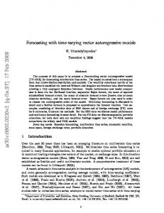
and the consistency with corresponding rate of convergence of this statistic are given in the following theorem. Theorem 3.1. Suppose that Assumptions 3.1-3.4 hold and define k ∗ := rn for some r ∈ (0, 1). Then, under the null hypothesis H0 , we have, as n → ∞, � βˆn,k∗ − β0 = Op n−1/2 . As seen from Theorem 3.1, Tn is not accurate for small k and n − k as the result does not hold if k/n = o(1) or (n − k)/n = o(1). In addition, the ELR statistic is not computable for small k and n − k. For this reason, we consider in the following discussion the trimmed and weighted-version of EL ratio test statistic, defined by �k� ˜ Pn,k , (3.1) Tn := 2 max h k1n ≤k≤k2n n where h is a given weight function, k1n := r1 n, k2n := r2 n and 0 < r1 < r2 < 1. If T˜n takes a significant large value, we have enough reason to reject the null hypothesis H0 of no change point. We also need a further assumption to control a remainder terms in the stochastic expansion of T˜n . Assumption 3.5. sup0 c) and c is the 95%-quantile of the sample {y0 , y1 , . . . , yn }. The trimming parameters in the definition of the statistic T˜n are chosen as r1n = 0.1 and r2n = 0.9. The critical value in ( 3.5) is obtained as the empirical 95% quantile of the Monte-Carlo samples � � �2 (l) (l) max B (k/n) − (k/n)B (1) : l = 1, . . . , 1000 , k1n ≤k≤k2n
where B (1) (·), . . . , B (1000) (·) are independent standard Brownian motions (note that in this case, the matrix in ( 3.3) is given by Q = 0). In Figures 1-3, we display the rejection probabilities of the ELR test ( 3.5) for the hypothesis ( 2.2), where the nominal level is chosen as α = 0.05. The horizontal and vertical axes show, respectively, the values of θ2 and the rejection rate of the hypothesis H0 : θ1 = θ2 at this point (θ1 is fixed as 0.3). The sample sizes are given by n = 100, 200 and 400 and the distribution of the innovation process is a standard normal distribution (Figure 1), a t-distribution with 2 degrees of freedom (Figure 2) and a Cauchy distribution (Figure 3). We also consider two values of the parameter r in the definition of the change point k ∗ = rn, that is r = 0.5 and r = 0.8. We observe that for small sample sizes, the test is slightly conservative and that the approximation of the nominal level improves with increasing sample size. The alternatives are rejected with reasonable probabilities, where the power is larger in the case r = 0.5 than for r = 0.8. A comparison of the different distributions in Figures 1-3 shows that the power is lower for standard normal distributed innovations, while 11
an error process with a Cauchy distribution yields the largest rejection probabilities. Other simulations show a similar picture, and the results are omitted for the sake of brevity. Figure 1: Simulated rejection probabilities of the ELR test ( 3.5) in the AR(1) model with normal distributed innovations. (a) θ1 = 0.3, r = 0.5
(b) θ1 = 0.3, r = 0.8
rejection rate
▮ △ ▮ △ ▮ △ ▮ △ ▮ ○ △ ○ ○ ○
▮
rejection rate
1.0
▮
▮
▮
△
△
○
0.6
▮
○ △0.4
○
▮
△
○
n = 100
△
n = 200
▮
n = 400
△ ○0.2
▮
▮
1.0
▮
▮
▮
○
0.8
0.6
○
○ -1.0
○
n = 100
△
n = 200
▮
n = 400 α = 0.05
△
▮
○
△
○ θ2
▮
0.4
△
○
○
1.0
△
▮
△
○
○
0.5
▮
▮ △
△
△ ○ △ ▮ ▮ ○ ○ △ ▮ ○ ○ △ △ ○ ○ -0.5
▮
△
α = 0.05
○
○
-1.0
▮ △
△
▮
○
▮ △
▮
0.8
△
▮ △
▮ △
▮
0.2▮ △ △ ○ ○ ○ △ ▮ ▮ △ ○ △ △ ▮ ▮ ○ ○ ○ △ ○ △ ○ △ ○ ○ ▮ 0.5
-0.5
1.0
θ2
Figure 2: Simulated rejection probabilities of the ELR test ( 3.5) in the AR(1) model with t-distributed innovations. (a) θ1 = 0.3, r = 0.5
(b) θ1 = 0.3, r = 0.8
rejection rate
▮ ▮ ▮ △ ○ △ ○ △ ▮ △ ▮ ○ △ ▮ △ ○ ○
▮ △
▮ △
○
rejection rate
1.0
▮
▮
▮ △
○
0.4
△
○ 0.2
○
△ ○
△ △ ▮ ▮ ○ △ △ ○ ○ ○ ▮ △ ○ 0.5
▮
▮
1.0
▮
○
n = 100
△
n = 200
▮
n = 400
○
△ 0.8
0.6
▮
△
○
▮ 0.4
△
○ ○
○ 1.0
-1.0
12
-0.5
○ △
○
▮
△
△ ▮ ○ △ ▮ △ ○ ○ ○ ▮ ▮ △ ○ △ ○ △ ○ ○ 0.5
○
n = 100
△
n = 200
▮
n = 400 α = 0.05
▮ △0.2
○ θ2
▮ △
△
○
▮
▮
○
α = 0.05
▮
▮ △
○
▮
▮ △
○
0.6
▮
▮ △
△
△
0.8
△
-0.5
▮ △ ○
▮ ▮
○
-1.0
▮ △
○
1.0
θ2
Figure 3: Simulated rejection probabilities of the ELR test ( 3.5) in the AR(1) model with Cauchy distributed innovations. (a) θ1 = 0.3, r = 0.5
(b) θ1 = 0.3, r = 0.8
rejection rate
▮ ▮ ▮ ▮ △ ○ △ ○ △ ○ △ ▮ △ ▮ ○ △ ▮ △ ○ ○
▮ △
▮1.0
rejection rate
▮
▮
△
○
▮ △
▮ ▮ △ △ ○ ○
▮ △
○
△ ○ △
0.6
○
○ 0.4
△
▮
○
-0.5
▮ △
▮ △
n = 100
△
n = 200
▮
n = 400
▮
1.0
▮
○
0.8
○ ○
○
0.6▮
△0.4
○
-1.0
△
▮
△
○ θ2
▮ △
△
○
1.0
▮ △
▮
○
0.5
▮
▮ △
○
△ ○ △
▮
△
α = 0.05
△ ○ ▮ ○ -1.0
○
▮
○ 0.2
▮ △
○
▮
0.8
▮ △
▮
△
▮ △
○
○
n = 100
△
n = 200
▮
n = 400 α = 0.05
○ △
0.2
▮ ○ △ ▮ △ ○ ○ ○ ○ △ △ ○ ▮ ○ ○
-0.5
0.5
1.0
θ2
In the second part of this section we compare the new test defined by ( 3.5) with the CUSUM test in Qu (2008) which uses quantile regression. The test statistic for the median in Qu (2008) is defined by ˆ − λH1,n (β)k, ˆ SQ0.5 = sup kHλ,n (β)
(4.1)
λ∈[0,1]
where k · k is the sup norm, βˆ is the median regressor, 0
−1/2
Hλ,n = (X X )
[λn] X
0 ˆ t−1 , |yt − Xt−1 β|X
i=1
and the matrix X is given by X = (X1 , . . . , Xn )0 . In Figures 4-6, we display the rejection probabilities of the test based on the statistic Tn in ( 2.5), T˜n in ( 3.1) and SQ0.5 in ( 4.1) for the hypothesis ( 2.2), where the nominal level is chosen as α = 0.05. The horizontal and vertical axes show, respectively, the values of θ2 and the rejection rate of the hypothesis H : θ1 = θ2 at this point (θ1 is fixed as 0.3). The distribution of the innovation process is a standard normal distribution (Figure 4), a t-distribution with 2 degree of freedom (Figure 5) and a Cauchy distribution (Figure 6) and the sample sizes are given by n = 100, 200 and 400 in each case. Again we consider two different locations for the change point k ∗ corresponding to the values r = 0.5 and r = 0.8. 13
We observe that all tests derived from the three statistics Tn in ( 2.5) (corresponding to the weight function h(r) ≡ 1), T˜n in ( 3.1) (corresponding to the weight function h(r) = r(1 − r)) and SQ0.5 in ( 4.1) are slightly conservative and that the approximation of the nominal level improves with increasing sample size [see Figure 4-6 for the value θ2 = θ1 = 0.3]. The approximation is usually more accurate for r = 0.5. Next we compare the power of the different tests (i.e. θ2 6= θ1 = 0.3) for different distributions of the innovations. In the case of Gaussian innovations all tests shows a similar behavior (see Figure 4) and only if the case n = 200 and r = 0.8 the ELR test based on the (unweighted) statistic Tn shows a better performance as the tests based on T˜n and SQ0.5 . Moreover, for Gaussian innovations all three tests show a remarkable robustness against non-stationarity, that is |θ2 | = 1. In Figure 5 we display corresponding results for t2 -distributed innovations. The differences in the approximation of the nominal level are negligible (θ2 = θ1 = 0.3). If r = 0.5 we do not observe substantial differences in the power between the three tests (independently of the sample size). On the other hand, if r = 0.8 the tests based on ELR statistics T˜n and Tn yield larger rejection probabilities than the test SQ0.5 (see the right part of Figure Figure 5). Interestingly the unweighted test based on Tn shows a better performance than the test based on T˜n in these cases. Again, all tests are robust with respect to non-stationarity. Finally, in Figure 6 we display the rejection probabilities of the three tests for Cauchy distributed innovations, where we again do not observe differences in the approximation of the nominal level (θ2 = θ1 = 0.3). On the other hand the differences in power between the tests based on ELR and quantile regression are remarkable. In all cases the ELR tests based on Tn and T˜n have substantially more power than the test based on SQ0.5 . The ELR test based on the unweighted statistic Tn shows a better performance than the ELR test based on T˜n . This superiority is less pronounced in the case r = 0.5 but clearly visible for r = 0.8. Finally, in contrast to the test based on SQ0.5 the ELR tests based on Tn and T˜n are robust against non-stationarity (i.e. |θ2 | = 1) for Cauchy distributed innovations and clearly detect a change in the parameters in these cases.
14
Figure 4: Simulated rejection probabilities of various change point tests based on the statistics Tn , T˜n and SQ0.5 defined in ( 2.5), ( 3.1) and ( 4.1), respectively. The model is given by an AR(1) model with normal distributed innovations. (i) n = 100 (a) r = 0.5
(b) r = 0.8
rejection rate 1.0
○ △ ○ △ ○ ▮ ▮ ▮ ▮ △ ○ △
rejection rate
▮ △
0.8
▮ ○ △
△
△ ▮ ○
0.4
˜ Tn
△
Tn
▮
SQ0.5
○
▮ △ ○
▮ △
○ ▮ △ ○ ▮ △ ○ ▮ △ ○
▮0.2 △ ○ ▮ △ ○ -1.0
0.5
-0.5
1.0
0.6
○ ▮ △
α = 0.05
▮
▮ ○ ▮ △ ▮ ○ ▮ ▮ △ ○ △ ▮ ○ ▮ △ ○ △ ○ △ ○ △ △
△
○ ○
0.6
▮ ○
0.8
○ ▮
θ2
-1.0
▮ 0.4
△
○
˜ Tn
△
Tn
▮
SQ0.5 α = 0.05
▮ ○ 0.2
△ ▮ ○ ▮ △ ○ ▮ △ ○ ○ ▮ ▮ ○ △ ▮ △ ▮ ▮ ▮ ○ ▮ △ ▮ △ ○ △ ○ △ ○ △ ○ △ ○ △ ○ 0.5
-0.5
1.0
θ2
(ii) n = 200 (a) r = 0.5
(b) r = 0.8
rejection rate
▮ △ ○ ○ ▮ ▮ △ ○ △ ○ ▮ △ ○ ▮ △
rejection rate
1.0
▮ ○ △
▮ ○
0.8
0.6
△
▮
▮ ○
○
▮ ○ ▮0.4 ○ ▮ ○ △
˜ Tn
△
1.0
△
△
Tn SQ0.5
θ2
-1.0
○
˜ Tn
△
Tn
▮
SQ0.5 α = 0.05
○ ▮ △ ▮ ○
0.2△
▮ ○
1.0
▮ ○
△0.4
▮ ○ ○ ▮
0.5
▮
△
△
-0.5
0.6
▮ ○
α = 0.05
▮ ▮ ○ ○ △ ▮ ▮ △ ○ ▮ △ ○ △ △ ○
△
0.8
△
▮ ○
0.2
△
△
▮ ○
▮
△
△
-1.0
△ △ △ △ ○ ▮ ○ ▮ ▮ ○
○ ▮ △
△ ▮ ○
○ △
△ ○ △ ○ ▮ ▮ ▮ ○ ○ ▮ ▮ △ ○ ▮ △ ○ △ ○ 0.5
-0.5
1.0
θ2
(iii) n = 400 (a) r = 0.5
(b) r = 0.8
rejection rate
▮ ▮ ▮ ▮ ▮ ○ △ ○ △ ○ △ ○ △ ○ △ ○ ▮ △ ○ ▮ △
rejection rate
1.0
△ ○ △ ○ △ ○ ○ ▮ ▮ △ △ ▮ ▮ ○ ▮ △ ○ ▮
○ △ ▮ ○ ▮ △
▮ ○ △
▮ ○
0.8
▮ ○
△
△0.6
▮ ○
▮ ○ 0.4
0.2
△
-0.5
˜ Tn
△
Tn
▮
SQ0.5
0.5
0.8
△
△0.4 ▮ ○
-1.0
15
-0.5
˜ Tn
△
Tn
▮
SQ0.5 α = 0.05
▮ △ ○ △ ○ ▮
1.0
○ △ ○
△ 0.2○ ▮
θ2
▮ △ ○
▮
0.6
▮ ○
▮ ○ △
▮ ○ △
△
▮ △ ○
○ ▮
α = 0.05
△
▮ ▮ ○ ○ △ ○ ▮ △ △ -1.0
○
1.0
▮ ▮ ○ △ ▮ △ ○ △ ○
▮ △ ○ 0.5
1.0
θ2
Figure 5: Simulated rejection probabilities of various change point tests based on the statistics Tn , T˜n and SQ0.5 defined in ( 2.5), ( 3.1) and ( 4.1), respectively. The model is given by an AR(1) model with t2 -distributed innovations. (i) n = 100 (a) r = 0.5
(b) r = 0.8
rejection rate
rejection rate
1.0
○ △ ○ △ ○ △ ○ ▮ △ ○ ▮ ▮ △ ○ ▮ ▮ ▮ △
△ ○ ○ △
0.8
○
○ 0.6
▮ ○ ▮ △ ○ △
△ ○ ▮ △
0.4
▮ ○
▮
▮
▮
△ ○ ▮
△
Tn
▮
SQ0.5
0.6
0.5
1.0
θ2
▮ △ ○
△ ○ ▮
α = 0.05
△ ○ ▮ △ ▮ △ ○ ▮ ○ △ △ ○ ▮ ○ △ △ ▮ △ ○
-0.5
0.8
△ ○
△ ○ ▮
▮ ○
0.2▮
-1.0
▮
˜ Tn
-1.0
▮
0.4
△ ○ ▮
○
˜ Tn
△
Tn
▮
SQ0.5 α = 0.05
▮ △ ○ △ ○ ▮
0.2
▮ △ ○
△ ▮ ○ ▮ ○ △ △ ○ ▮ ○ ▮ ▮ ▮ ○ ▮ △ △ ○ ▮ △ ○ △ ○ △ △ ○ 0.5
-0.5
1.0
θ2
(ii) n = 200 (a) r = 0.5
(b) r = 0.8
rejection rate
rejection rate
1.0
△ ○ △ ○ △ ○ ○ △ ○ △ ○ △ ○ ▮ ▮ ▮ ▮ ▮ △ ▮ ▮ ○ ▮
○ △ ○ ▮ △
0.8
△ ▮ ○
0.6
▮
▮ ○
△ ▮ ○ △ 0.2
▮ ○ △
▮
○
˜ Tn
△
Tn
▮
SQ0.5
△
0.4
-1.0
▮
△ ○ △ △ △ △ ○ ○ ▮ ○ ▮
○ △
△
1.0
△
△0.6
▮
△
▮ ○ ▮
▮ ○
0.4
○ ▮
△ ▮ ▮ ○ ○ △ △ ○ ▮ △
-0.5
0.5
1.0
θ2
0.8
▮ ○
○
α = 0.05
-1.0
△ ○ ▮
△
○ ▮
△
△
▮
○
˜ Tn
△
Tn
▮
SQ0.5
○
△
α = 0.05
▮ △ ○0.2 ○ ▮ △ ○ ▮ ▮ ○ ▮ ▮ △ ○ ▮ △ ▮ ○ △ ○ ○ 0.5
-0.5
1.0
θ2
(iii) n = 400 (a) r = 0.5
(b) r = 0.8
rejection rate
○ △ ○ △ ○ △ ○ △ ○ △ ○ △ ○ △ ○ ▮ △ ▮ ▮ ▮ ▮ ▮ ▮ ▮
rejection rate
1.0
○ ▮ △ 0.8
▮ ○ △
▮
○ 0.6△
○
˜ Tn
△
Tn
▮
SQ0.5
▮ ▮ ○
0.4
-1.0
-0.5
△ ○ △ ▮ ○ ▮ △ ○ ▮
0.8
▮ △ ○
▮ ○ ▮0.4△
▮ ○ △
▮ ○ △
0.2
▮ ○ △ 0.5
1.0
▮ △ ○
△ ▮ ○ ▮ ▮ ○ △ △ ○ △ ○ ▮
θ2
-1.0
16
-0.5
○
˜ Tn
△
Tn
▮
SQ0.5 α = 0.05
○ ▮
△ 0.2
1.0
△0.6
α = 0.05
△
○
○ △ ○ △ ○ △ ○ △ ○ △ △ ▮ ▮ ○ △ ▮ ○ ▮ ▮ △ ▮ ○ ▮
△ △ ○ ○ △ ○ ▮ ▮ ▮
0.5
1.0
θ2
Figure 6: Simulated rejection probabilities of various change point tests based on the statistics Tn , T˜n and SQ0.5 defined in ( 2.5), ( 3.1) and ( 4.1), respectively. The model is given by an AR(1) model with Cauchy distributed innovations. (i) n = 100 (a) r = 0.5
(b) r = 0.8
rejection rate
rejection rate
1.0
○ △ ○ △ ○ △ ○ ○ △ △ ○ △ ○
○ △
0.8
△ ○
○ △
○
△ ○
○
△ 0.6
▮ ▮
▮
▮
▮
0.4
△
▮ ▮
-1.0
○
△ ○ ▮
△ ▮
○
▮0.2△ ○ ▮ △ ▮
▮
˜ Tn
0.8
△ ○ △
△
Tn SQ0.5
○ △
▮ ▮
α = 0.05
▮
○
▮ ▮
△ ○ ▮ △ ▮ ○ ▮ △ ○ ▮ △ 0.5
1.0
θ2
-1.0
▮
▮
△ ○
0.4
○ △
○ ▮
-0.5
△ ○ 0.6
○ △
▮ ▮
△ ○
△ ○ ▮
○
˜ Tn
△
Tn
▮
SQ0.5
▮
α = 0.05
△ ○
△ ▮ 0.2 ○ △ ▮ △ ○ ○ ○ ○ △ ▮ ▮ △ ○ △ ▮ ▮ ▮ ○ ▮ △ ▮ △ ○ ▮ 0.5
-0.5
1.0
θ2
(ii) n = 200 (a) r = 0.5
(b) r = 0.8
rejection rate
△ ○ △ ○ △ ○ △ ○ △ ○ ○ △ ○ △ ○ △
rejection rate
1.0
○ △
○ △
△ △ ○ ○ △ ○
△ ○ △ ○ △ △ △ △ ○ ○ ○
0.8
○
▮
▮
▮
▮
▮
0.6△
▮ ▮
▮
△
○
▮0.4 ▮
△ ○ △ ▮
▮
0.2
-1.0
○
○ ▮ △
▮ ▮
▮
▮
△
Tn
▮
SQ0.5
1.0
1.0
0.8
○
▮
△
○
△
0.6
▮
○
▮
△
▮
-1.0
▮
0.2
▮
˜ Tn
△
Tn
▮
SQ0.5 α = 0.05
▮ ○
○
▮
○
▮
○0.4
▮ ▮
△ ○
○
△
○
θ2
△ △
△
▮
0.5
-0.5
˜ Tn
α = 0.05
○ △ ▮
△
○
○
▮
△
▮
△
▮
▮ ○ △ ○ ○ ▮ ▮ ○ △ ▮ ▮ 0.5
-0.5
1.0
θ2
(iii) n = 400 (a) r = 0.5
(b) r = 0.8
rejection rate
rejection rate
△ ○ △ ○ △ ○ △ ○ △ ○ △ ○ △ ○ △ ○ ○ △1.0 ○ △
○ △
△ ○ △ ○ △ ○ △ ○
△ ○ △ ○ △ ○ △ ○ △ ○ ○ △ ○ △ △ ○
○
0.8
△ ▮ ▮
▮
▮
▮
▮
▮
▮
0.6
▮
▮
▮
▮ 0.4
▮
▮ ▮
○
▮ ○ ▮ △
˜ Tn
△
Tn
▮
SQ0.5
○ ▮
△
▮ ▮
1.0
θ2
0.4
▮ ▮
-1.0
17
▮
△
-0.5
▮ ▮
○
▮ ▮
0.5
▮
△ ○
0.6○
▮
α = 0.05
△ ▮
○ △ ▮ -0.5
△ △ ○ △ ○ ○ △ ○
0.8
○
0.2
-1.0
1.0
△
0.2
▮
▮
▮
△ ○ ▮
△ ○ ▮
˜ Tn
△
Tn
▮
SQ0.5 α = 0.05
▮
△ ○ ▮ 0.5
○
1.0
θ2
5
Proofs
This section gives rigorous proofs of all results in this paper. In what follows, C will denote a generic positive constant that varies in different places. “with probability approaching one” will be abbreviated as w.p.a.1. Moreover, we use the following notations throughout this section: gi (β) = g(Yi p , β),
g(β) = E[g(Yi p , β)],
k
1X Pˆk1 (β, λ) = log{1 − λ0 gi (β)}, k i=1 2 Pˆn,k (β, η) =
n X 1 log{1 − η 0 gj (β)}, n − k j=k+1
ˆ 1 (β) = {λ ∈ Rm : |λ0 gi (β)| < 1 for all i = 1, . . . , k} , Λ k ˆ 2n,k (β) = {η ∈ Rm : |η 0 gj (β)| < 1 for all j = k + 1, . . . , n} , Λ n
n
1X 1X g(Yi p , β) = gi (β), gˆ(β) = n i=1 n i=1 k
gˆk1 (β)
5.1
1X = gi (β) k i=1
and
2 gˆn,k (β)
n X 1 gj (β). = n − k j=k+1
Proof of Theorem 3.1
We start proving several auxiliary results which are required in the proof of Theorem 3.1. Lemma 5.1. Suppose that Assumption 3.4 (i) holds. For 1/γ < ζ < 1/2, let Λn,k = {(λ, η) ∈ R2m : kλk ≤ Ck −ζ ,
kηk ≤ C(n − k)−ζ }.
Then, as n → ∞, we have sup β∈B,λ∈Λn,k∗
P
max |λ0 gi (β)| − → 0,
1≤i≤k∗
sup β∈B,η∈Λn,k∗
ˆ 1 ∗ (β) × Λ ˆ 2 ∗ (β) for all β ∈ B w.p.a.1. Also, Λn,k∗ ⊂ Λ k n,k 18
max
k∗ +1≤j≤n
P
|η 0 gj (β)| − → 0.
Proof. Let bi = supβ∈B kgi (β)k. By Assumption 3.4 (i), we can choose γ > 2 such that K = E[bγ1 ]1/γ is finite. Then, for any δ > 0, we can define M (δ) = K/δ 1/γ and obtain ∗
P
�
max∗ bi ≥ M (δ)k
∗ 1/γ
1≤i≤k
�
≤
k X
∗
�
P bi ≥ M (δ)k
∗ 1/γ
�
=
i=1
≤
k∗ X i=1
k X
P (bγi ≥ M (δ)γ k ∗ )
i=1
E[bγi ] = δ. M (δ)γ k ∗
Consequently, maxi bi = Op (k ∗ 1/γ ) and by the Cauchy-Schwartz inequality we have sup β∈B,λ∈Λn,k∗
max |λ0 gi (β)| ≤ sup kλk max∗ bi = Op (k ∗ −ζ+1/γ ),
1≤i≤k∗
1≤i≤k
λ∈Λn,k∗
which implies sup
P
max∗ |λ0 gi (β)| − → 0.
β∈B,λ∈Λn,k∗ 1≤i≤k
Similarly, it follows that sup β∈B,η∈Λn,k∗
max
k∗ +1≤j≤n
P
|η 0 gj (β)| − → 0.
ˆ 1 ∗ (β) × Λ ˆ 2 ∗ (β) for all β ∈ B w.p.a.1, which completes the proof Therefore, Λn,k∗ ⊂ Λ k n,k of Lemma 5.1. Lemma 5.2. Suppose that Assumptions 3.1 – 3.4 hold, and there exists a sequence {β n,k∗ } ⊂ B such that P
∗ −1/2 2 β n,k∗ − → β0 , gˆk1∗ (β n,k∗ ) = Op (k ∗ −1/2 ) and gˆn,k ) ∗ (β n,k ∗ ) = Op ((n − k )
as n → ∞. Denote β n,k∗ by β. Then, under H0 , λ := arg max Pˆk1∗ (β, λ) ˆ 1 ∗ (β) λ∈Λ k
and
η := arg
max
ˆ 2 ∗ (β) η∈Λ n,k
2 Pˆn,k ∗ (β, η)
exist w.p.a.1. Moreover, as n → ∞ we have λ = Op (k ∗ −1/2 ), η = Op ((n − k ∗ )−1/2 ), 2 ∗ −1 Pˆk1∗ (β, λ) = Op (k ∗ −1 ), Pˆn,k ). ∗ (β, η) = Op ((n − k ) 19
Proof. We only show the statement for λ, the corresponding statement for η follows by similar arguments. Since Λn,k∗ is a closed set, it follows that ˇ := arg max Pˆ 1∗ (β, λ) λ k λ∈Λn,k∗
exists (note that Pˆk∗ (β, λ) is a concave function of λ). From Lemma 5.1 it follows that Pˆk1∗ (β, λ) is continuously twice differentiable with respect to λ w.p.a.1. By a ˇ and 0m such Taylor expansion at λ = 0m , there exists a point λ˙ on the line joining λ that ˇ 0 = Pˆk1∗ (β, 0m ) ≤ Pˆk1∗ (β, λ) k∗ h1 X i 1 1 ˙ 0 ˇ ˇ 0 gˆ1∗ (β) + λ ˇ0 = −λ ρ (β) λ, ( λ)g (β)g i i k 2 k ∗ i=1 i
(5.1)
where ρ1i (λ) = −1/(1 − λ0 gi (β))2 . Note that the definition of gi (β) implies 1 gi (β)gi (β)0 = a∗ (Xi−1 )a∗ (Xi−1 )0 4 ˙ ≥ −C uniformly with respect to for any β ∈ B. By Lemma 5.1 we have ρ1i (λ) i w.p.a.1. Furthermore, the ergodicity of {Xt : t ∈ Z} implies that the random variable k∗ X 1 ∗ −1 ˆ Ωk∗ := (4k ) a∗ (Xi−1 )a∗ (Xi−1 )0 i=1
ˆ 1 ∗ is bounded converges to Ω in probability. Hence the minimum eigenvalue of Ω k away from 0 w.p.a.1. and we obtain ∗
k i 1 ˇ0h 1 X 1 ˙ C ˇ ˆ1 ˇ 0 1 ˇ ˇ ≤ kλk ˇ kˆ −λ gˆk∗ (β) + λ ∗ ρi (λ)gi (β)gi (β)0 λ gk1∗ (β)k − λ Ωk∗ λ 2 k i=1 2
ˇ g 1∗ (β)k − Ckλk ˇ 2 ≤ kλkkˆ k ˇ we get w.p.a.1. Dividing both sides of ( 5.2) by kλk, ˇ = Op (k ∗ −1/2 ) = op (k ∗ −ζ ), kλk 20
(5.2)
ˇ ∈ Int(Λ ˆ 1 ∗ ) w.p.a.1. Again by Lemma 5.1, the concavity of Pˆ 1∗ (β, λ) and hence λ k k 1 ˇ ˆ and the convexity of Λk∗ (β), it follows that λ = λ exists w.p.a.1 and λ = Op (k ∗ −1/2 ). These results also imply that Pˆk1∗ (β, λ) = Op (k ∗ −1 ). By similar arguments, we can 2 show the corresponding results for η and Pˆn,k ∗ (β, η). Next, let us consider the estimator βˆn,k of Theorem 3.1. Recall that βˆn,k is the minimizer of ln,k (β, β) = k sup Pˆk1 (β, λ) + (n − k) ˆ 1 (β) λ∈Λ k
sup ˆ 2 (β) η∈Λ n,k
2 Pˆn,k (β, η).
Let us define 2 Pˆn,k (β, λ, η) := k Pˆk1 (β, λ) + (n − k)Pˆn,k (β, η)
(5.3)
and ˆ n,k := arg λ
max
ˆ 1 (βˆn,k ) λ∈Λ k
Pˆk1 (βˆn,k , λ),
ηˆn,k := arg
max
ˆ 2 (βˆn,k ) η∈Λ n,k
2 Pˆn,k (βˆn,k , η).
(5.4)
Lemma 5.3. Suppose that Assumptions 3.1 – 3.4 hold. Then, under the null hypothesis H0 of no change point we have 2 ∗ −1/2 ˆ gˆk1∗ (βˆn,k∗ ) = Op (k ∗ −1/2 ), gˆn,k ) ∗ (βn,k ∗ ) = Op ((n − k )
as n → ∞. l Proof. Define gˆˆn,k := gˆl (βˆn,k ) for l = 1, 2,
˜ n,k := −k −1/2 gˆˆ1 /kgˆˆ1 k, λ n,k n,k
2 2 η˜n,k := −(n − k)−1/2 gˆˆn,k /kgˆˆn,k k,
(5.5)
then it follows from ( 5.4) that ˜ n,k ) ≤ Pˆ 1 (βˆn,k , λ ˆ n,k ) and Pˆ 2 (βˆn,k , η˜n,k ) ≤ Pˆ 2 (βˆn,k , ηˆn,k ), Pˆk1 (βˆn,k , λ n,k k n,k which implies the inequality ˜ n,k , η˜n,k ) ≤ Pˆn,k (βˆn,k , λ ˆ n,k , ηˆn,k ). Pˆn,k (βˆn,k , λ
21
(5.6)
By similar arguments as used in ( 5.1) and ( 5.2) we have ˜ n,k∗ , η˜n,k∗ ) ≥ k ∗ 1/2 kgˆˆ1 ∗ k + (n − k ∗ )1/2 kgˆˆ2 ∗ k − c0 Pˆn,k∗ (βˆn,k∗ , λ n,k n,k
(5.7)
w.p.a.1, where c0 is the same constant as in the proof of Lemma 5.2. On the other hand, we have the following inequality: ˆ n,k , ηˆn,k ) = inf Pˆn,k (βˆn,k , λ
β∈B
≤
Pˆn,k (β, λ, η)
sup ˆ 1 (βˆn,k ), η∈Λ ˆ 2 (βˆn,k ) λ∈Λ k n,k
Pˆn,k (β0 , λ, η)
sup ˆ 1 (β0 ), η∈Λ ˆ 2 (β0 ) λ∈Λ k n,k
≤ k sup Pˆk1 (β0 , λ) + (n − k) ˆ 1 (β0 ) λ∈Λ k
sup ˆ 2 (β0 ) η∈Λ n,k
2 Pˆn,k (β0 , η).
(5.8)
Applying Lemma 5.2 with β n,k∗ = β0 yields sup ˆ 1 ∗ (β0 ) λ∈Λ k
Pˆk1∗ (β0 , λ) = Op (k ∗ −1 ),
sup ˆ 2 ∗ (β0 ) η∈Λ n,k
2 ∗ −1 Pˆn,k ), ∗ (β0 , η) = Op ((n − k )
(5.9)
and from ( 5.8) and ( 5.9), we get ˆ n,k∗ , ηˆn,k∗ ) = Op (1). Pˆn,k∗ (βˆn,k∗ , λ
(5.10)
Finally, from ( 5.6), ( 5.7) and ( 5.10), we have 1 ∗ 1/2 ˆ2 ˆ n,k∗ , ηˆn,k∗ ) = Op (1), −c0 ≤ −c0 + k ∗ 1/2 kgˆˆn,k kgˆn,k∗ k ≤ Pˆn,k∗ (βˆn,k∗ , λ ∗ k + (n − k )
which implies 1 2 2 ∗ −1/2 ˆ kgˆˆn,k gk1∗ (βˆn,k∗ )k = Op (k ∗ −1/2 ) and kgˆˆn,k gn,k ), ∗ k = kˆ ∗ (βn,k ∗ )k = Op ((n−k ) ∗ k = kˆ
establishing the assertion of Lemma 5.3. Proof. [Proof of Theorem 3.1] By Lemma 5.3 we have gˆ(βˆn,k∗ ) = op (1). Then, it follows from the triangular inequality and uniform law of large numbers that kg(βˆn,k∗ )k ≤ kg(βˆn,k∗ ) − gˆ(βˆn,k∗ )k + kˆ g (βˆn,k∗ )k 22
≤ sup kg(β) − gˆ(β)k + kˆ g (βˆn,k∗ )k = op (1). β∈B
Since g(β) has a unique zero at β0 , the function kg(β)k must be bounded away from zero outside any neighborhood of β0 . Therefore, βˆn,k∗ must be inside any P neighborhood of β0 w.p.a.1. and therefore, βˆn,k∗ − → β0 . Next, we show that βˆn,k∗ − β0 = Op (n−1/2 ). As k ∗ = rn, by Lemma 5.3, we have n o 2 ˆ gˆ(βˆn,k∗ ) = n−1 k ∗ gˆk1∗ (βˆn,k∗ ) + (n − k ∗ )ˆ gn,k = Op (n−1/2 ) ∗ (βn,k ∗ ) and the central limit theorem implies h n oi gˆ(β0 ) = Op n−1 k ∗ 1/2 + (n − k ∗ )1/2 = Op (n1/2 ). Further, kˆ g (βˆn,k∗ ) − gˆ(β0 ) − g(βˆn,k∗ )k ≤ (1 +
√ nkβˆn,k∗ − β0 k)op (n−1/2 ),
(5.11)
which yields kg(βˆn,k∗ )k ≤ kˆ g (βˆn,k∗ ) − gˆ(β0 ) − g(βˆn,k∗ )k + kˆ g (βˆn,k∗ )k + kˆ g (β0 )k h n oi √ = (1 + nkβˆn,k∗ − β0 k)op (n−1/2 ) + Op n−1 k ∗ 1/2 + (n − k ∗ )1/2 . Moreover, similar arguments as given in Newey and McFadden (1994) on page 2191, the differentiability of kg(β)k and the estimate kg(βˆn )k ≥ Ckβˆn − β0 k w.p.a.1. show that h n oi √ kβˆn,k∗ − β0 k = (1 + nkβˆn,k∗ − β0 k)op (n−1/2 ) + Op n−1 k ∗ 1/2 + (n − k ∗ )1/2 , and hence h n oi {1 + op (1)}kβˆn,k∗ − β0 k = op (n−1/2 ) + Op n−1 k ∗ 1/2 + (n − k ∗ )1/2 .
(5.12)
If k ∗ = rn the right-hand side of ( 5.12) is of order Op (n−1/2 ), which completes the proof of Theorem 3.1.
23
5.2
Proof of Theorem 3.2
We first show that Pˆn,k∗ (β, λ, η) in ( 5.3) is well approximated by some function near its optima using a similar reasoning as in Parente and Smith (2011). For this purpose let us define ˆ 1 (β, λ) = {−G(β − β0 ) − gˆ1 (β0 )}0 λ − 1 λ0 Ωλ, L k k 2 2 2 0 ˆ (β, η) = {−G(β − β0 ) − gˆ (β0 )} η − 1 η 0 Ωη L n,k n,k 2 and ˆ n,k (β, λ, η) := k L ˆ 1 (β, λ) + (n − k)L ˆ 2 (β, η). L k n,k Furthermore, hereafter redefine β˜n,k := arg min
sup
β∈B λ∈Rm ,η∈Rm
˜ n,k := arg max L ˜ λ) ˆ 1 (β, λ k m λ∈R
ˆ n,k (β, λ, η), L and
˜ η). ˆ 2 (β, η˜n,k := arg max L n,k m η∈R
Lemma 5.4. Suppose that Assumptions 3.1-3.4 hold. Then, under H0 , ˜ n,k∗ , η˜n,k∗ ) + op (1) ˆ n,k∗ , ηˆn,k∗ ) = L ˆ n,k∗ (β˜n,k∗ , λ Pˆn,k∗ (βˆn,k∗ , λ as n → ∞. Proof. It is sufficient to show that ˆ n,k∗ , ηˆn,k∗ ) − L ˆ n,k∗ , ηˆn,k∗ ) = op (1), ˆ n,k∗ (βˆn,k∗ , λ (i) Pˆn,k∗ (βˆn,k∗ , λ ˆ n,k∗ , ηˆn,k∗ ) − L ˆ n,k∗ , ηˆn,k∗ ) = op (1), ˆ n,k∗ (βˆn,k∗ , λ ˆ n,k∗ (β˜n,k∗ , λ (ii) L ˆ n,k∗ , ηˆn,k∗ ) − L ˜ n,k∗ , η˜n,k∗ ) = op (1). ˆ n,k∗ (β˜n,k∗ , λ ˆ n,k∗ (β˜n,k∗ , λ (iii) L For a proof of (i) we note that a Taylor expansion leads to k
i 1 ˆ0 h 1 X 1 ¨ ∗ 0 ˆ1 1 ˆ ∗ 0 ˆ ˆ ˆ ˆ Pk (βn,k , λn,k ) = −λn,k gˆn,k + λn,k ρ (λ)a (Xi−1 )a (Xi−1 ) λn,k , 2 k i=1 i
24
¨ is on the line joining the points λ ˆ n,k and 0m . Observing the definition of where λ ˆ n,k ) this yields the estimate ˆ 1 (βˆn,k , λ L � �0 ˆ1 ˆ ˆ ˆ n,k ) ≤ − gˆˆ1 − gˆ1 (β0 ) − G(βˆ − β0 ) λ ˆ n,k (5.13) ˆ 1 (βˆn,k , λ Pk (βn,k , λn,k ) − L n,k k 1 h k i ˆ0 1 X 1 ∗ ∗ 0 ˆ + λn,k ρ˙ i a (Xi−1 )a (Xi−1 ) + Ω λn,k . 2 k i=1 P Since βˆn,k∗ − → β0 by Theorem 3.1, we can take β n,k∗ = βˆn,k∗ in Lemma 5.2, and ˆ n,k∗ = Op (n−1/2 ). Then, recalling ( 5.11), the first term in ( 5.13) (where k obtain λ is replaced by k ∗ ) becomes � �0 1 ˆ n,k∗ ˆk1∗ (β0 ) − G(βˆn,k∗ − β0 ) λ − gˆˆn,k ∗ − g
o
n
1
ˆ
ˆ 1 ˆ ˆ ∗ ∗ ∗ ∗ ≤ gˆˆn,k − g ˆ λ (β ) − g( β ) + g( β ) − G( β − β )
n,k ∗ 0 n,k n,k 0 n,k k∗
n� � � �o √
2 = 1 + n βˆn,k∗ − β0 op (n−1/2 ) + Op βˆn,k∗ − β0 Op (n−1/2 )
=op (n−1 ). Moreover, the second term in ( 5.13) is of order op (k ∗ −1 ). Hence, we get 1 ˆ n,k∗ ) − L ˆ n,k∗ ) = op (k ∗ −1 ) ˆ 1 (βˆn,k , λ Pˆk∗ (βˆn,k∗ , λ and similarly 2 ˆ 2 (βˆn,k∗ , ηˆn,k∗ ) = op ((n − k ∗ )−1 ). Pˆn,k∗ (βˆn,k∗ , ηˆn,k∗ ) − L Combining these estimates yields ˆ n,k∗ , ηˆn,k∗ ) − L ˆ n,k∗ , ηˆn,k∗ ) = op (1), ˆ n,k∗ (βˆn,k∗ , λ Pˆn,k∗ (βˆn,k∗ , λ which is the statement (i). For a proof of (ii) we first show ˆ n,k∗ , ηˆn,k∗ ) = op (1). ˆ n,k∗ , ηˆn,k∗ ) − L ˆ n,k∗ (β˜n,k∗ , λ Pˆn,k∗ (β˜n,k∗ , λ ˆ n,k (β, λ, η) is smooth in β, λ and η. Then, the first order Note that the function L conditions for an interior global maximum 0p =
ˆ n,k (β, λ, η) ∂L = −G0 {kλ + (n − k)η} , ∂β 25
ˆ n,k (β, λ, η) � ∂L = −k G(β − β0 ) + gˆk1 (β0 ) + Ωλ , ∂λ ˆ � ∂ Ln,k (β, λ, η) 2 0m = = −(n − k) G(β − β0 ) + gˆn,k (β0 ) + Ωη ∂η 0m =
0 ˜ 0 , η˜0 ). These conditions can be ,λ are satisfied for the point (β 0 , λ0 , η 0 ) = (β˜n,k n,k n,k rewritten in matrix form as Op×p G0 G0 β˜n,k − β0 0p 1 ˜ n,k k −1 Ω Om×m kλ G + gˆk (β0 ) = 0p+2m . (5.14) 2 G Om×m (n − k)−1 Ω (n − k)˜ ηn,k gˆn,k (β0 )
With the notations Σ := (G0 Ω−1 G)−1 , H := Ω−1 GΣ, n−k k 2 := Ω−1 − HΣ−1 H 0 , Pk1 := Ω−1 − HΣ−1 H 0 , Pn,k n n the system ( 5.14) is equivalent to β˜n,k − β0 ˜ n,k kλ (n − k)˜ ηn,k 0p n−1 Σ −kn−1 H 0 −(n − k)n−1 H 0 = −kn−1 H −kPk1 k(n − k)n−1 HΣ−1 H 0 gˆk1 (β0 ) 2 2 gˆn,k (β0 ) −(n − k)n−1 H k(n − k)n−1 HΣ−1 H 0 −(n − k)Pn,k −H 0 gˆ(β0 ) = (5.15) −k {Ω−1 gˆk1 (β0 ) − HΣ−1 H 0 gˆ(β0 )} . � −1 2 −(n − k) Ω gˆn,k (β0 ) − HΣ−1 H 0 gˆ(β0 ) ˜ n,k∗ and η˜n,k∗ are of order Op (n−1/2 ), Op (k ∗ −1/2 ) and Consequently, β˜n,k∗ − β0 , λ Op ((n − k ∗ )−1/2 ), respectively. Therefore, by the same arguments as given in the proof of (i), it follows that ˆ n,k∗ , ηˆn,k∗ ) − L ˆ n,k∗ , ηˆn,k∗ )| = op (1). ˆ n,k∗ (β˜n,k∗ , λ |Pˆn,k∗ (β˜n,k∗ , λ
26
0 0 0 0 0 ˆ0 ˜0 ˜0 This relationship and the fact that (βˆn,k ˆn,k ˜n,k ∗ , λn,k ∗ , η ∗ ) and (βn,k ∗ , λn,k ∗ , η ∗ ) are the ˆ n,k∗ (β, λ, η), respectively, imply that saddle points of the functions Pˆn,k∗ (β, λ, η) and L
ˆ n,k∗ , ηˆn,k∗ ) = Pˆn,k∗ (βˆn,k∗ , λ ˆ n,k∗ , ηˆn,k∗ ) + op (1) ˆ n,k∗ (βˆn,k∗ , λ L ˆ n,k∗ , ηˆn,k∗ ) + op (1) ≤ Pˆn,k∗ (β˜n,k∗ , λ ˆ n,k∗ , ηˆn,k∗ ) + op (1). ˆ n,k∗ (β˜n,k∗ , λ =L
(5.16)
On the other hand, ˆ n,k∗ , ηˆn,k∗ ) ≤ L ˜ n,k∗ , η˜n,k∗ ) ˆ n,k∗ (β˜n,k∗ , λ ˆ n,k∗ (β˜n,k∗ , λ L ˜ n,k∗ , η˜n,k∗ ) ˆ n,k∗ (βˆn,k∗ , λ ≤L ˜ n,k∗ , η˜n,k∗ ) + op (1) = Pˆn,k∗ (βˆn,k∗ , λ ˆ n,k∗ , ηˆn,k∗ ) + op (1) ≤ Pˆn,k∗ (βˆn,k∗ , λ ˆ n,k∗ , ηˆn,k∗ ) + op (1). ˆ n,k∗ (βˆn,k∗ , λ =L
(5.17)
Thus, ( 5.16) and ( 5.17) lead to ˆ n,k∗ , ηˆn,k∗ ) − L ˆ n,k∗ , ηˆn,k∗ ) = op (1). ˆ n,k∗ (βˆn,k∗ , λ ˆ n,k∗ (β˜n,k∗ , λ L Finally, we can prove (iii) by similar arguments that ˜ n,k∗ , η˜n,k∗ ) ≤ L ˜ n,k∗ , η˜n,k∗ ) ˆ n,k∗ (β˜n,k∗ , λ ˆ n,k∗ (βˆn,k∗ , λ L ˜ n,k∗ , η˜n,k∗ ) + op (1) = Pˆn,k∗ (βˆn,k∗ , λ ˆ n,k∗ , ηˆn,k∗ ) + op (1) ≤ Pˆn,k∗ (βˆn,k∗ , λ ˆ n,k∗ , ηˆn,k∗ ) + op (1) ≤ Pˆn,k∗ (β˜n,k∗ , λ ˆ n,k∗ , ηˆn,k∗ ) + op (1) ˆ n,k∗ (β˜n,k∗ , λ =L and ˆ n,k∗ , ηˆn,k∗ ) ≤ L ˜ n,k∗ , η˜n,k∗ ). ˆ n,k∗ (β˜n,k∗ , λ ˆ n,k∗ (β˜n,k∗ , λ L ˆ n,k∗ , ηˆn,k∗ ) = L ˜ n,k∗ , η˜n,k∗ )+op (1), which implies ˆ n,k∗ (β˜n,k∗ , λ ˆ n,k∗ (β˜n,k∗ , λ Consequently, L (iii).
27
Proof. [Proof of Theorem 3.2] By ( 5.3), ( 5.4), Lemma 5.4 and ( 5.15) it follows that ˆ n,k∗ , ηˆn,k∗ ) sup{−ln,k∗ (β, β)} = Pˆn,k∗ (βˆn,k∗ , λ β∈B
˜ n,k∗ , η˜n,k∗ ) + Rn,k∗ ˆ n,k∗ (β˜n,k∗ , λ =L ∗ k∗ ˜0 ˜ n,k∗ + n − k η˜0 ∗ Ω˜ Ω λ ηn,k∗ + Rn,k∗ + op (1) = λ ∗ n,k 2 n,k 2 k∗ n − k∗ 2 2 = gˆk1∗ (β0 )0 Ω−1 gˆk1∗ (β0 ) + gˆn,k∗ (β0 )0 Ω−1 gˆn,k ∗ (β0 ) 2 2 n − gˆ(β0 )0 HΣ−1 H 0 gˆ(β0 ) + Rn,k∗ + op (1) 2 ˆ = Mn,k∗ + Rn,k∗ + op (1), (5.18) where ˆ n,k M
ˆ n (k/n) − (k/n)W ˆ n (1) 2 W
W ˆ n (1)0 QW ˆ n (1) = + , 2φ(k/n) 2 [rn]
X ˆ n (r) = √1 Ω−1/2 g(Yt p , β0 ), W n t=1 ˆ n,k , ηˆn,k ) − L ˜ n,k , η˜n,k ), ˆ n,k (β˜n,k , λ Rn,k = Pˆn,k (βˆn,k , λ φ(u) = u(1 − u) and [x] denotes the integer part of real number x. As shown in Lemma 5.4, max |Rn,k∗ | = sup |Rn,rn | = op (1). ∗ k1n ≤k ≤k2n
r1 ≤r≤r2
Second, from Assumption 3.4 and Lemma 2.2 in Phillips (1987), it follows that n o L ˆ n (r) : r ∈ [0, 1] − c0 W → {c0 B(r) : r ∈ [0, 1]} , for any vector c ∈ Rm , where {B(r) : r ∈ [0, 1]} is an m-dimensional standard Brownian motion. Hence, the Cram´er-Wold device and the continuous mapping theorem lead to n �k� o ˆ n,k M T˜n = 2 max h k1n ≤k≤k2n n n h(k/n) o
ˆ n (r) − ([rn]/n)W ˆ n (1) 2 + h([rn]/n)W ˆ n (1)0 QW ˆ n (1)
W = sup k1n /n≤r≤k2n /n φ(k/n) 28
L
− → sup r1 ≤r≤r2
5.3
n h(r) φ(r)
o kB(r) − rB(1)k + h(r)B(1) QB(1) . 2
0
Proof of Theorem 3.3
Proof. Without loss of generality, suppose that θ2 6= β0 . This implies that there exist a neighborhood U (β0 ) of β0 and a neighborhood U (θ2 ) of θ2 such that U (β0 ) ∩ U (θ2 ) = ∅. Under the alternative it follows that βˆn,k∗ 6∈ U (β0 ) or βˆn,k∗ 6∈ U (θ2 ). Note that E[g(Ytp , θ2 )] 6= 0 for 1 ≤ t ≤ k ∗ and E[g(Ytp , β0 )] 6= 0 for k ∗ + 1 ≤ t ≤ n. From a 2 ˆ uniform law of large numbers, gˆk1∗ (βˆn,k∗ ) or gˆn,k ∗ (βn,k ∗ ) is outside a neighborhood of 0 for any sufficiently large n. 2 2 Now, if we consider gˆk1 (βˆn,k∗ ) instead of gˆk1 (β0 ) and gˆn,k (βˆn,k∗ ) instead of gˆn,k (β0 ) in ( 5.14), we find, as in ( 5.18), that supβ∈B {−ln,k∗ (β, β)} can be approximated by n − k∗ 2 k∗ 1 ˆ 2 ˆ gˆk∗ (βn,k∗ )0 Ω−1 gˆk1∗ (βˆn,k∗ ) + gˆn,k∗ (βˆn,k∗ )0 Ω−1 gˆn,k ∗ (βn,k ∗ ) 2 2 n − gˆ(βˆn,k∗ )0 HΣ−1 H 0 gˆ(βˆn,k∗ ) + Rn,k∗ + op (1). 2 This time, however, we have k∗ 1 ˆ n − k∗ 2 2 ˆ gˆk∗ (βn,k∗ )0 Ω−1 gˆk1∗ (βˆn,k∗ ) + gˆn,k∗ (βˆn,k∗ )0 Ω−1 gˆn,k ∗ (βn,k ∗ ) → ∞, 2 2 2 0 −1 2 ˆ since gˆk1∗ (βˆn,k∗ )0 Ω−1 gˆk1∗ (βˆn,k∗ ) + gˆn,k gˆn,k∗ (βˆn,k∗ ) > 0 for any sufficiently ∗ (βn,k ∗ ) Ω large n. This completes the proof of Theorem 3.3.
Acknowledgements. The authors would like to thank Martina Stein who typed this manuscript with considerable technical expertise. The work of authors was supported by JSPS Grant-in-Aid for Young Scientists (B) (16K16022), Waseda University Grant for Special Research Projects (2016S-063) and the Deutsche Forschungsgemeinschaft (SFB 823: Statistik nichtlinearer dynamischer Prozesse, Teilprojekt A1 and C1). 29
References Andrews, D. W. (1993). Tests for parameter instability and structural change with unknown change point. Econometrica: Journal of the Econometric Society 61 (4), 821–856. Aue, A. and L. Horv´ ath (2013). Structural breaks in time series. Journal of Time Series Analysis 34 (1), 1–16. Bai, J. (1993). On the partial sums of residuals in autoregressive and moving average models. Journal of Time Series Analysis 14, 247–260. Bai, J. (1994). Convergence of the sequential empirical processes of residuals in ARMA models. Annals of Statistics 22 (4), 2051–2061. Baragona, R., F. Battaglia, D. Cucina, et al. (2013). Empirical likelihood for break detection in time series. Electronic Journal of Statistics 7, 3089–3123. Berkes, I., Horv´ ath, S. Ling, and J. Schauer (2011). Testing for structural change of AR model to threshold AR model. Journal of Time Series Analysis 32 (5), 547–565. Chen, K., Z. Ying, H. Zhang, and L. Zhao (2008). Analysis of least absolute deviation. Biometrika 95 (1), 107–122. Chuang, C.-S. and N. H. Chan (2002). Empirical likelihood for autoregressive models, with applications to unstable time series. Statistica Sinica 12, 387–407. Ciuperca, G. and Z. Salloum (2015). Empirical likelihood test in a posteriori change-point nonlinear model. Metrika 78, 919–952. Cressie, N. and T. R. Read (1984). Multinomial goodness-of-fit tests. Journal of the Royal Statistical Society. Series B (Methodological) 46 (3), 440–464. Cs¨org¨o, M. and L. Horv´ ath (1997). Limit Theorems in Change-Point Analysis. John Wiley. Davis, R. A., D. Huang, and Y.-C. Yao (1995). Testing for a change in the parameter values and order of an autoregressive model. Annals of Statistics 23 (1), 282–304. Gombay, E. and L. Horv´ ath (1990). Asymptotic distributions of maximum likelihood tests for change in the mean. Biometrika 77 (2), 411–414. Lee, S., J. Ha, O. Na, and S. Na (2003). The cusum test for parameter change in time series models. Scandinavian Journal of Statistics 30 (4), 781–796. Ling, S. (2005). Self-weighted least absolute deviation estimation for infinite variance autoregressive models. Journal of the Royal Statistical Society: Series B (Statistical Methodology) 67 (3), 381–393. Newey, W. K. and D. McFadden (1994). Large sample estimation and hypothesis testing.
30
Handbook of Econometrics 4, 2111–2245. Nolan, J. P. (2015). Stable Distributions - Models for Heavy Tailed Data. Boston: Birkhauser. In progress, Chapter 1 online at academic2.american.edu/∼jpnolan. Owen, A. B. (1988). Empirical likelihood ratio confidence intervals for a single functional. Biometrika 75 (2), 237–249. Page, E. S. (1954). Continuous inspection schemes. Biometrika 41 (1/2), 100–115. Page, E. S. (1955). Control charts with warning lines. Biometrika 42(1-2), 243–257. Pan, J., H. Wang, and Q. Yao (2007). Weighted least absolute deviations estimation for ARMA models with infinite variance. Econometric Theory 23 (05), 852–879. Parente, P. M. and R. J. Smith (2011). GEL methods for nonsmooth moment indicators. Econometric Theory 27 (01), 74–113. Phillips, P. C. (1987). Time series regression with a unit root. Econometrica 55 (2), 277– 301. Qin, J. and J. Lawless (1994). Empirical likelihood and general estimating equations. The Annals of Statistics 22 (1), 300–325. Qu, Z. (2008). Testing for structural change in regression quantiles. Journal of Econometrics 146 (1), 170–184. Samoradnitsky, G. and M. S. Taqqu (1994). Stable non-Gaussian Random Processes: Stochastic Models with Infinite Variance, Volume 1. CRC Press. Su, L. and Z. Xiao (2008). Testing for parameter stability in quantile regression models. Statistics & Probability Letters 78 (16), 2768–2775. Zhou, M., H. J. Wang, and Y. Tang (2015). Sequential change point detection in linear quantile regression models. Statistics & Probability Letters 100, 98–103.
31