Change-Point Detection in Time-Series Data by Relative Density-Ratio Estimation Song Liu1 , Makoto Yamada2 Nigel Collier3 , and Masashi Sugiyama1 1 Tokyo Institute of Technology 2-12-1 O-okayama, Meguro-ku, Tokyo 152-8552, Japan, {song@sg., sugi@}cs.titech.ac.jp, 2 NTT Communication Science Laboratories 2-4, Hikaridai, Seika-cho, Kyoto, Japan 619-0237,
[email protected] 3 National Institute of Informatics 2-1-2 Hitotsubashi, Chiyoda-ku, Tokyo 101-8430, Japan,
[email protected]
Abstract. The objective of change-point detection is to discover abrupt property changes lying behind time-series data. In this paper, we present a novel statistical change-point detection algorithm that is based on nonparametric divergence estimation between two retrospective segments. Our method uses the relative Pearson divergence as a divergence measure, and it is accurately and efficiently estimated by a method of direct density-ratio estimation. Through experiments on real-world humanactivity sensing, speech, and Twitter datasets, we demonstrate the usefulness of the proposed method. Keywords: change-point detection, distribution comparison, relative density-ratio estimation, kernel methods, time-series data
1
Introduction
Detecting abrupt changes in time-series data, called change-point detection, has attracted researchers in the statistics and data mining communities for decades [1–6]. Some pioneer works demonstrated good change-point detection performance by comparing the probability distributions of time-series samples over past and present intervals [1]. As both the intervals move forward, a typical strategy is to issue an alarm for a change point when the two distributions are becoming significantly different. Various change-point detection methods follow this strategy, for example, the cumulative sum [1], the generalized likelihood-ratio method [2], and the change finder [3]. Another group of methods that have attracted high popularity in recent years is the subspace methods [4, 5]. By using a pre-designed time-series model, a subspace is discovered by principle component analysis from trajectories in past and present intervals, and their dissimilarity is measured by the distance
Y(t + n).
Y(t)
Y (t + n − 1)
e
f
g
j
k
n Y (t + 1) Y (t) a
b
c
b
c
a
b
c
k
l
Y (t + 2n − 1) d
g
h
f
g
h
f
g
h
i
Y−(t + n + 1) Y (t + n) Fig. 1. Notation.
b
e
i
j
k
l
Time
y(t)
y(t + n)
between the subspaces. One of the major approaches is called subspace identification [5], which compares the subspaces spanned by the columns of an extended observability matrix generated by a state-space model with system noise. However, the methods explained above rely on pre-designed parametric models such as underlying probability distributions [1, 2], auto-regressive models [3], and state-space models [4, 5], for tracking some specific statistics such as the mean, the variance, and the spectrum. Thus, they are not robust against different types of changes, which significantly limits the range of applications in practice. To cope with this problem, non-parametric estimation methods such as kernel density estimation may be used. However, non-parametric methods tend to be less accurate in high-dimensional problems because of the so-called curse of dimensionality. To overcome this difficulty, a new strategy was introduced recently which estimates the ratio of probability densities directly without going through density estimation [7]. In the context of change-point detection, a direct density-ratio estimation method called the Kullback-Leibler importance estimation procedure (KLIEP) [8] was reported to outperform competitive approaches [6] such as the one-class support vector machine [9] and singular-spectrum analysis [4]. The goal of this paper is to further advance this line of research. More specifically, our contributions in this paper are two folds. • We apply a recently-proposed density-ratio estimation method called the unconstrained least-squares importance fitting (uLSIF) [10] to change-point detection. Notable advantages of uLSIF are that an analytical solution can be obtained, it achieves the optimal non-parametric convergence rate, it has optimal numerical stability, and it has higher robustness [7]. • We further improve the uLSIF-based change-point detection method by employing a state-of-the-art extension of uLSIF called relative uLSIF (RuLSIF) [11], which was proved to have an even better non-parametric convergence property than plain uLSIF [11], with other advantages of uLSIF maintained.
2
Problem Formulation
In this section, we formulate our change-point detection problem (see Figure 1). Let y(t) ∈ Rd be a d-dimensional time-series sample at time t. Let Y (t) := [y(t)⊤ , y(t + 1)⊤ , . . . , y(t + k − 1)⊤ ]⊤ ∈ Rdk
be a subsequence of time series at time t with length k, where ⊤ represents the transpose. Following the previous work [6], we treat the subsequence Y (t) as a sample, instead of a single point y(t), by which time-dependent information can be incorporated naturally. Let Y(t) be a set of n retrospective subsequence samples starting at time t: Y(t) := {Y (t), Y (t + 1), . . . , Y (t + n − 1)}. For change-point detection, let us consider two consecutive segments Y(t) and Y(t+n). Our strategy is to compute a certain dissimilarity measure between Y(t) and Y(t + n), and use it as the plausibility of change points. More specifically, the larger the dissimilarity is, the more likely the point is a change point. Now the problems that need to be addressed are what kind of dissimilarity measure we should use and how we estimate it from data. We will discuss these issues in the next section.
3
Change-Point Detection via Density-Ratio Estimation
In this section, we first define our dissimilarity measure, and then show methods for estimating the dissimilarity measure. 3.1
Divergence-Based Dissimilarity Measure
We use a dissimilarity measure of the following form: D(Pt ∥Pt+n ) + D(Pt+n ∥Pt ),
(1)
where Pt and Pt+n are probability distributions of samples in Y(t) and Y(t + n), respectively. D(P ∥P ′ ) denotes the f -divergence [12, 13]: ( ) ∫ p(Y ) ′ ′ D(P ∥P ) := p (Y )f dY , p′ (Y ) where f is a convex function such that f (1) = 0, and p(Y ) and p′ (Y ) are probability density functions of P and P ′ , respectively. Because the f -divergence is not symmetric, we use a symmetrized divergence in Eq.(1). The f -divergence includes various popular divergences such as the KullbackLeibler (KL) divergence by f (t) = t log t and the Pearson (PE) divergence by f (t) = 12 (t − 1)2 : ( )2 ∫ ∫ p(Y ) 1 ′ p(Y ) ′ ′ KL(P ∥P ) := p(Y ) log ′ dY and PE(P ∥P ) := p (Y ) ′ −1 dY . p (Y ) 2 p (Y ) In the rest of this section, we explain three methods of directly estimating ) ′ n n the density ratio pp(Y ′ (Y ) from samples {Y i }i=1 and {Y j }j=1 drawn from p(Y ) and p′ (Y ): the KL importance estimation procedure (KLIEP) [8] in Section 3.2, unconstrained least-squares importance fitting (uLSIF) [10] in Section 3.3, and relative uLSIF (RuLSIF) [11] in Section 3.4.
3.2
Kullback-Leibler Importance Estimation Procedure (KLIEP)
KLIEP [8] is a direct density-ratio estimation algorithm that is suitable for estimating the KL divergence. Density-Ratio Model: Let us model the density ratio kernel model: g(Y ; θ) :=
n ∑
p(Y ) p′ (Y )
by the following
θℓ K(Y , Y ℓ ),
(2)
ℓ=1
where θ := (θ1 , . . . , θn )⊤ are parameters to be learned from data samples, and K(Y , Y ′ ) is a kernel basis function. In practice, we use the Gaussian kernel and the kernel width is chosen by cross-validation (see [8] for details). Learning Algorithm: The parameters θ in the model g(Y ; θ) are determined so that the empirical KL divergence from p(Y ) to g(Y ; θ)p′ (Y ) is minimized: ( n ) n n n ∑ 1∑ 1∑∑ max log θℓ K(Y i , Y ℓ ) s.t. θℓ K(Y ′j ,Y ℓ ) = 1, θ1 , . . . , θn ≥ 0. θ n n i=1 j=1 ℓ=1
ℓ=1
The equality constraint is for normalization purposes because g(Y ; θ)p′ (Y ) should be a probability density function. The inequality constraint comes from the non-negativity of the density-ratio function. Since this is a convex optimizab can be simply obtained, for tion problem, the unique global optimal solution θ example, by a gradient-projection iteration. Finally, a density-ratio estimator is given as gb(Y ) =
n ∑
θbℓ K(Y , Y ℓ ).
(3)
ℓ=1
KLIEP was shown to achieve the optimal non-parametric convergence rate [8]. Change-Point Detection by KLIEP: Given a density-ratio estimator gb(Y ), an approximator of the KL divergence is given as ∑ c := 1 KL log gb(Y i ). n i=1 n
In the previous work [6], this KLIEP-based KL-divergence estimator was applied to change-point detection and demonstrated to be promising in experiments. 3.3
Unconstrained Least-Squares Importance Fitting (uLSIF)
Recently, another direct density-ratio estimator called uLSIF was proposed [10], which is suitable for estimating the PE divergence.
Learning Algorithm: In uLSIF, the same density-ratio model g(Y ; θ) as KLIEP (see Eq.(2)) is used. However, its training criterion is different; the density-ratio model is fitted to the true density ratio under the squared loss. More specifically, the parameter θ in the model g(Y ; θ) is determined so that the following squared loss J(Y ) is minimized: )2 ∫ ( 1 p(Y ) J(Y ) := − g(Y ; θ) p′ (Y ) dY 2 p′ (Y ) ∫ ∫ ∫ 2 1 p(Y ) ′ 1 = g(Y ; θ)2 p′ (Y ) dY . p (Y ) dY − p(Y )g(Y ; θ) dY + 2 p′ (Y ) 2 Since the first term is a constant, we focus on the last two terms. By approximating the expectations by the empirical averages, the uLSIF optimization problem is given as follows: [ ] 1 c b ⊤ θ + λ θ⊤ θ , −h (4) minn θ ⊤ Hθ θ∈R 2 2 where the penalty term λ2 θ ⊤ θ is included for regularization purposes, and λ (≥ 0) denotes the regularization parameter, which is chosen by cross validation. b is the n-dimensional vector c is the n × n matrix and h (see [10] for details). H defined as n n ∑ 1∑ b ℓ,ℓ′ := 1 H K(Y ′j , Y ℓ )K(Y ′j , Y ℓ′ ) and b hℓ := K(Y i , Y ℓ ). n j=1 n i=1 b of (4) can be analytically obtained as It is easy to confirm that the solution θ b = (H b c + λI n )−1 h, θ
(5)
where I n denotes the n-dimensional identity matrix. Finally, a density-ratio estimator is given by Eq.(3) with Eq.(5). Change-Point Detection by uLSIF: Given a density-ratio estimator gb(Y ), an approximator of the PE divergence can be constructed as ∑ 1∑ 1 c := − 1 PE gb(Y ′j )2 + gb(Y i ) − . 2n j=1 n i=1 2 n
n
This approximator is derived from the following expression of the PE divergence: )2 ) ∫ ( ∫ ( p(Y ) p(Y ) 1 1 ′ ′ p (Y )dY + p(Y )dY − . (6) PE(P ∥P ) = − 2 p′ (Y ) p′ (Y ) 2 Notable advantages of uLSIF are that its solution can be computed analytically, it possesses the optimal non-parametric convergence rate, it has the optimal numerical stability, and it has higher robustness [7]. As experimentally demonstrated in our supplementary technical report [14], uLSIF-based changepoint detection compares favorably with the KLIEP-based method.
3.4
Relative uLSIF (RuLSIF)
Depending on the condition of the denominator density p′ (Y ), the density-ratio ) value pp(Y ′ (Y ) can be unbounded (i.e., they can be infinity). This is actually problematic because the non-parametric convergence rate of uLSIF is governed by ) the “sup”-norm of the true density-ratio function: maxY pp(Y ′ (Y ) . To overcome this problem, relative density-ratio estimation was introduced [11]. Relative PE Divergence: Let us consider the α-relative PE-divergence for 0 ≤ α < 1: ∫ 2 ′ ′ PEα (P ∥P ) := PE(P ∥αP + (1 − α)P ) = p′α (Y ) (rα (Y ) − 1) dY , ) where p′α (Y ) = αp(Y ) + (1 − α)p′ (Y ) and rα (Y ) = pp(Y ′ (Y ) . We refer to rα (Y ) as α the α-relative density ratio. The α-relative density ratio is reduced to the plain density ratio if α = 0, and it tends to be “smoother” as α gets larger. Indeed, the α-relative density ratio is bounded above by 1/α for α > 0, even when the plain ) density ratio pp(Y ′ (Y ) is unbounded. This was proved to contribute to improving the estimation accuracy [11].
Learning Algorithm: In the same way as the uLSIF method, the parameter θ of the model g(Y ; θ) is learned by minimizing the squared difference between true and estimated ratios: ∫ 1 J(Y ) = p′α (Y )(rα (Y ) − g(Y ; θ))2 dY 2 ∫ ∫ 1 = p′α (Y )rα2 (Y )dY − p(Y )rα (Y )g(Y ; θ) dY 2 ∫ ∫ 1−α α 2 p(Y )g(Y ; θ) dY − p′ (Y )g(Y ; θ)2 dY , + 2 2 where the first term is a constant term. Note that we still use the same kernel model (2) as g(Y ; θ) for approximating the α-relative density ratio. Again, by ignoring the constant and approximating the expectations by empirical averages, the α-relative density ratio can be learned in the same way as the plain density ratio. Indeed, the optimization problem of a relative variant of uLSIF, called RuLSIF, is given as the same form as uLSIF; the only difference c which is now given by is the definition of the matrix H, ∑ (1 − α) ∑ b ℓ,ℓ′ := α H K(Y i , Y ℓ )K(Y i , Y ℓ′ ) + K(Y ′j , Y ℓ )K(Y ′j , Y ℓ′ ). n i=1 n j=1 n
n
RuLSIF inherits the advantages of uLSIF, i.e., its solution can be computed analytically, it has the superior numerical stability, and it has higher robustness; furthermore, RuLSIF possesses an even better non-parametric convergence property than uLSIF [11].
Change-Point Detection by RuLSIF: By using an estimator gb(Y ) of the α-relative density ratio, the α-relative PE divergence can be approximated as ∑ 1−α ∑ 1∑ 1 c α := − α gb(Y i )2 − gb(Y ′j )2 + gb(Y i ) − . PE 2n i=1 2n j=1 n i=1 2 n
n
n
As experimentally demonstrated in our supplementary technical report [14], the RuLSIF-based change-point detection performs even better than the plain uLSIF-based method. Thus, we focus on RuLSIF in the experiments in Section 4.
4
Experiments
In this section, we experimentally investigate the performance of the proposed and existing change-point detection methods. First, we use a human activity dataset and a speech dataset. The human activity dataset is a subset of the Human Activity Sensing Consortium (HASC) challenge 2011, which provides human activity information collected by portable three-axis accelerometers. The speech dataset is the IPSJ SIG-SLP Corpora and Environments for Noisy Speech Recognition (CENSREC) dataset provided by National Institute of Informatics (NII), which records human voice in a noisy environment. We compare our RuLSIF-based method with several state-of-theart methods: Singular spectrum transformation (SST) [4], subspace identification (SI) [5], auto regressive (AR) [3], and one-class support vector machine (OSVM) [9]. Examples of RuLSIF-based change score and ROC curves over 10 datasets are plotted in Figures 2 and 3, showing that the proposed RuLSIF-based method outperforms other methods. Finally, we apply the proposed change-point detection method to the CMU Twitter dataset, which is an archive of Twitter messages that have been collected from April 2010 to October 2010 via the Twitter API. Here we track the degree of popularity of a given topic by monitoring the frequency of selected keywords. More specifically, we focus on events related to “Deepwater Horizon oil spill in the Gulf of Mexico” which occurred on April 20, 2010, and was widely broadcast among the Twitter community. We use the frequency of 10 keywords: “gulf ”, “spill ”, “bp”, “oil ”, “hayward ”, “mexico”, “coast”, “transocean”, “halliburton”, and “obama” (see Figure 4(a)). For quantitative evaluation, we referred to the Wikipedia entry “Timeline of the Deepwater Horizon oil spill” as a real-world event source. The change-point score obtained by the proposed RuLSIF-based method is plotted in Figure 4(b), where four occurrences of important real-world events show the development of this news story. As we can see from Figure 4(b), the change-point score increases immediately after the initial explosion of the deepwater horizon oil platform and soon reaches the first peak when oil was found on the sea shore of Louisiana on April 30. Shortly after BP announced its preliminary estimation on the amount of leaking oil, the change-point score rises quickly again and reaches its second peak at the end of May, at which time President Obama visited Louisiana to assure local
4 3
1
2
0.8 1 0 0
500
1000
1500
0.6
2000
0.4
0.4
RuLSIF SST SI AR OSVM
0.3
0.2 0.2 0.1
0
0 0
500
1000
1500
0
2000
(a) One of the original time-series and RuLSIF-based change score
0.2
0.4
0.6
0.8
1
(b) Average ROC curves
Fig. 2. HASC human-activity dataset (http://hasc.jp/hc2011/). 0.1
1 0.05 0
0.8
−0.05
0.6
−0.1 0
500
1000 1500 2000 2500 3000 3500 4000 4500 5000
0.4
0.12
RuLSIF SST SI AR OSVM
0.1 0.08
0.2
0.06 0.04
0
0.02 0 0
500
0
1000 1500 2000 2500 3000 3500 4000 4500 5000
(a) One of the original time-series and RuLSIF-based change score
0.2
0.4
0.6
0.8
1
(b) Average ROC curves
Fig. 3. NII speech dataset (http://research.nii.ac.jp/src/eng/list/index.html). gulf
1
1
0.5
spill
0.5
0 May mexico
1
Aug
Feb 1
0.5
Aug
May
Aug
Feb
May Aug transocean
0.5
Aug
Feb 1
0 May Aug halliburton
May
Aug
Feb
Feb 1
May obama
Aug
May
Aug
0.5
0
Feb
hayward
0.5
0.5
0 May
1
0
Feb 1
0
Feb
oil
0.5
0 May coast
0.5
0
1
0.5
0
Feb
bp
1
0 May
Aug
Feb
(a) Normalized frequencies of 10 keywords 0.4
Oil Reaches Mainland, Apr 30
0.35
BP Cuts Off Oil Spill, Obama Visits Louisiana, Jul 15 May 28 BP Stock at 1−year Low, Jun 25
0.3 0.25 0.2 0.15
Initial Explosion, Apr 20
0.1 0.05 0 Feb 1
Mar 1
Apr 1
May 1
Jun 1
July 1
Aug 1
(b) RuLSIF-based change score and exemplary real-world events Fig. 4. Twitter dataset (http://www.ark.cs.cmu.edu/tweets/).
residents of the federal government’s support. On June 25, the BP stock was at its one year’s lowest price, while the change-point score spikes at the third time. Finally, BP cuts off the spill on July 15, as the score reaches its last peak.
5
Conclusion
We extended the existing KLIEP-based change detection method and proposed to use uLSIF or RuLSIF as a building block. Through experiments, we demonstrated that the RuLSIF-based change detection method is promising. SL was supported by NII internship fund and the JST PRESTO program. MY and MS were supported by the JST PRESTO program. NC was supported by NII Grand Challenge project fund.
References 1. Basseville, M., Nikiforov, I.V.: Detection of Abrupt Changes: Theory and Application. Prentice-Hall, Inc., Upper Saddle River, NJ, USA (1993) 2. Gustafsson, F.: The marginalized likelihood ratio test for detecting abrupt changes. IEEE Transactions on Automatic Control 41(1) (1996) 66–78 3. Takeuchi, Y., Yamanishi, K.: A unifying framework for detecting outliers and change points from non-stationary time series data. IEEE Transactions on Knowledge and Data Engineering 18(4) (2006) 482–489 4. Moskvina, V., Zhigljavsky, A.: Change-point detection algorithm based on the singular-spectrum analysis. Communications in Statistics: Simulation and Computation 32 (2003) 319–352 5. Kawahara, Y., Yairi, T., Machida, K.: Change-point detection in time-series data based on subspace identification. In: Proceedings of the 7th IEEE International Conference on Data Mining. (2007) 559–564 6. Kawahara, Y., Sugiyama, M.: Sequential change-point detection based on direct density-ratio estimation. Statistical Analysis and Data Mining 5(2) (2012) 114–127 7. Sugiyama, M., Suzuki, T., Kanamori, T.: Density Ratio Estimation in Machine Learning. Cambridge University Press, Cambridge, UK (2012) 8. Sugiyama, M., Suzuki, T., Nakajima, S., Kashima, H., von Buenau, P., Kawanabe, M.: Direct importance estimation for covariate shift adaptation. Annals of the Institute of Statistical Mathematics 60(4) (2008) 699–746 9. Desobry, F., Davy, M., Doncarli, C.: An online kernel change detection algorithm. IEEE Transactions on Signal Processing 53(8) (2005) 2961–2974 10. Kanamori, T., Hido, S., Sugiyama, M.: A least-squares approach to direct importance estimation. Journal of Machine Learning Research 10 (2009) 1391–1445 11. Yamada, M., Suzuki, T., Kanamori, T., Hachiya, H., Sugiyama, M.: Relative density-ratio estimation for robust distribution comparison. In: Advances in Neural Information Processing Systems 24. (2011) 594–602 12. Ali, S.M., Silvey, S.D.: A general class of coefficients of divergence of one distribution from another. Journal of the Royal Statistical Society, Series B 28(1) (1966) 131–142 13. Csisz´ ar, I.: Information-type measures of difference of probability distributions and indirect observation. Studia Scientiarum Mathematicarum Hungarica 2 (1967) 229–318 14. Liu, S., Yamada, M., Collier, N., Sugiyama, M.: Change-point detection in timeseries data by relative density-ratio estimation. arXiv 1203.0453 (2012)